Cosmological perturbations through a simple bounce

Abstract

We present a detailed study of a simple scalar field model that yields non-singular cosmological solutions. We study both the qualitative dynamics of the homogeneous and isotropic background and the evolution of inhomogeneous linear perturbations. We calculate the spectrum of perturbations generated on super-Hubble scales during the collapse phase from initial vacuum fluctuations on small scales and then evolve these numerically through the bounce. We show there is a gauge in which perturbations remain well-defined and small throughout the bounce, even though perturbations in other commonly used gauges become large or ill-defined. We show that the comoving curvature perturbation calculated during the collapse phase provides a good estimate of the resulting large scale adiabatic perturbation in the expanding phase while the Bardeen metric potential is dominated by what becomes a decaying mode after the bounce. We show that a power-law collapse phase with scale factor proportional to $(-t)^{2/3}$ can yield a scale-invariant spectrum of adiabatic scalar perturbations in the expanding phase, but the amplitude of tensor perturbations places important constraints on the allowed initial conditions.

I Introduction

Current cosmological observations, especially measurements of the spectrum of temperature anisotropies and polarisation of the cosmic microwave background, provide strong evidence for the existence of primordial density perturbations on large scales, far larger than the Hubble scale at the time of last-scattering. Observations are consistent with an almost scale-invariant, Gaussian distribution of adiabatic primordial perturbations WMAP .

The standard explanation for the origin of the primordial perturbations is that the Universe underwent an accelerated, inflationary, expansion in the early universe LLbook . Zero-point vacuum fluctuations in a massless scalar field naturally give rise to a scale-invariant distribution of effectively classical field fluctuations on super-Hubble scales during an exponential (de Sitter) expansion. If inflation is driven by a light, slowly-rolling, inflaton field then these field fluctuations can be directly related to a comoving curvature perturbation, ${\cal{R}}$, which remains constant for adiabatic perturbations on super-Hubble scales until a given wavelength re-enters the horizon in the subsequent radiation- or matter-dominated eras.

It is important to consider whether or not inflation is the only consistent model for the origin of large-scale structure in our Universe. An alternative proposal is that the hot big bang and the primordial perturbations originate not from an accelerated expansion, but from a preceding collapse. In classical general relativity a collapsing universe may be doomed to a singularity, but in a finite quantum theory of gravity, such as string theory, the spectrum of states going into the “singularity” would be expected to determine some out-going state. In particular the collapse phase could set the initial conditions for a subsequent post-big bang phase. Gasperini and Veneziano originally proposed GV a pre big bang scenario based on the superstring low energy effective action pbbreviews . More recently Khoury et al proposed the ekpyrotic scenario ekpyrotic motivated by colliding brane solutions in heterotic M-theory (see also pyro ; cyclic for later developments of this scenario). Both models invoke a collapsing universe in the 4D Einstein frame where the energy density is dominated by minimally coupled scalar fields.

In a collapsing universe zero-point vacuum fluctuations with a given wavelength are squeezed outside the rapidly shrinking Hubble scale, also naturally giving rise to a spectrum of field fluctuations on super-Hubble scales. However in either pre big bang or ekpyrotic scenarios, vacuum fluctuations give rise to a steeply blue-tilted spectrum of comoving curvature perturbations during the collapse BGGMV ; Lyth . If the tilt of the comoving curvature spectrum remains unchanged during the transition from pre to post big bang phase then this cannot seed the observed large scale structure in our Universe. One would then have to consider alternative sources for structure after a collapse phase, such as the curvaton mechanism curvaton , or consider a different collapse model. Collapse driven by matter or a scalar field with pressureless equation of state can produce a scale-invariant spectrum of comoving curvature perturbations Wands99 ; FB .

Although very general physical arguments have been advanced that the comoving curvature perturbation, ${\cal{R}}$, should be conserved on super-horizon scales for adiabatic density perturbations Lyth85 ; DM ; MS ; WMLL ; LW03 there are several possible ambiguities that may arise in the transition from collapse to bounce, not present in conventional models of an inflationary expansion. At any bounce the comoving Hubble scale diverges and all scales are inside the Hubble scale, at least for an instant MP . And the Bardeen metric potential, $\Phi$, does not have the same spectral dependence as the comoving curvature perturbation during the collapse BF ; Hwang ; Khoury2 ; Lyth2 ; HwangNoh ; DV , even though the two tilts must coincide for adiabatic perturbations in the subsequent expanding universe. As a result it is impossible for both ${\cal{R}}$ and $\Phi$ to obey non-singular evolution equations through the bounce CDC .

In fact the Bardeen potential on super-Hubble scales grows rapidly in a collapsing phase. This was noted in Ref. BGGMV who realised that the divergence of perturbations in the Bardeen’s longitudinal (or conformal Newtonian) gauge could be eliminated by a gauge-transformation to the spatially flat (or off-diagonal) gauge. However we will see that at the moment of bounce the spatially flat gauge itself becomes ill-defined. The comoving curvature perturbation may remain small during collapse but it too becomes ill-defined in the vicinity of the bounce in our model. The breakdown of perturbation theory in any given gauge does not necessarily signal the breakdown of perturbation theory. It is well known that the comoving curvature perturbation becomes singular at stationary values of the field even in single-field inflation models, but there are other gauge choices where perturbations remain small Kodama .

Several authors have studied the evolution of perturbations through a bounce using some analytic form for the background scale factor PPN ; PPNG ; Finelli:2003mc and/or the evolution equations for perturbations CDC . But this has lead to apparently contradictory results depending on which functions are assumed to have a smooth regular form CDC .

In order to investigate some of these issues associated with the evolution of cosmological perturbations through the bounce we will consider a simple scalar field model for a non-singular bounce. We are following the general approach envisaged in the pre big bang scenario GV where higher-order corrections to the effective action will become significant at high curvatures or strong coupling and can yield non-singular bounce solutions nonsing ; Ed . In the ekpyrotic or cyclic models the transition is supposed to occur at a real singularity in the effective-4D theory. Not only background quantities but also perturbations diverge here. So our 4D analysis will not address arguments about the regularisation schemes at the singularity proposed so far Khoury2 ; Schwarz ; Tolley .

There have already been a few numerical studies of the evolution of perturbations through non-singular bounce solutions including higher-order corrections to the string effective action Tsujikawa:2001ad ; Tsujikawa:2002qc ; CartierHwang ; Cartier . It can be shown that that the null energy condition must be violated for a bounce to occur in general relativity in a spatially flat 4D FRW cosmology Brustein . (This is quite different from non-singular classical bounces which have been studied in closed FRW models ParkerFulling ; Starobinsky78 ; Matzner ; Hwangbounce ; GordonTurok ; Deruelle ; DeruelleStreich ; MP which do not violate the null energy condition, but require fine-tuned initial conditions to obtain a sufficiently long collapse phase Starobinsky78 ; Matzner .) One problem with results based on higher-order corrections near the bounce is that the evolution close to the bounce becomes dominated by the “corrections” and one cannot be sure that even higher-order corrections would not also become important Ed . Another complication is that increasingly higher-order corrections are equivalent to introducing additional fields with non-canonical kinetic terms TT ; Wands93 so that the true dynamical degrees of freedom become obscured.

In order to make the physical degrees of freedom manifest we will work with scalar fields obeying canonical wave equations in four-dimensional Einstein gravity. The price we must pay for such simplicity, while still obtaining a non-singular bounce, is that one of the scalar fields will be a massless “ghost” field with negative kinetic energy, in order to violate the null energy condition near the bounce. Such a ghost field would lead to the presence of serious instabilities in any low energy theory ghosts . However it does not play any significant role in our model at early or late times. Instead it leads to precisely the sort of instability at high energies that we require to achieve a bounce in the high-energy regime, destabilising the pre big bang collapse phase and triggering the transition to an expanding cosmology. Our scalar field model is intended only as a simple model of a non-singular bounce and not as a realistic model of the low energy universe. The early- and late-time (low energy) evolution in our model is dominated by a conventional minimally-coupled scalar field with exponential potential. By choosing the dimensionless slope of the potential we are able to investigate different power-law solutions for the pre big bang collapse leading to different power spectra for the field and metric perturbations Wands99 . A very similar bounce model was studied by Peter and Pinto-Neto PPN , but we find very different results.

In the original pre big bang scenario higher-order corrections to the effective action will become significant at high curvatures or strong coupling and can yield non-singular bounce solutions nonsing ; Ed , at least for some initial conditions and some higher-order corrections. In particular it can be shown that the null energy condition must be violated for a bounce to occur in a 4D FRW cosmology Brustein .

We first study the background evolution of our model using a phase-plane analysis in Section II. With a particular choice of dimensionless phase variables the early or late time solutions correspond to critical points in the phase plane. However an alternative choice of variables is better suited to study evolution through the bounce. We identify a class of non-singular models which start in a power-law collapse in the asymptotic past, pass smoothly through a bounce and approach a power-law expansion.

We then define linear perturbations about this background model in Section III. We present the evolution and constraint equations for the perturbations in arbitrary gauge and then identify particular gauge choices that are well-suited to study the perturbations at early and late times, or through the bounce, analogously to the different choice of background variables used to study the background phase-plane in different regimes. The choice of gauge to take the perturbations through the bounce is vital as it must be ensured that the gauge itself is well defined throughout the bounce, and we identify problems with gauges commonly used in inflationary models.

In section IV we evolve first-order evolution equations for the metric and field perturbations and use the constraint equations as a consistency check of our calculation. We assume perturbations begin in the quantum vacuum state on small scales and use this to calculate the spectrum of perturbations generated on super-Hubble scales during collapse. We evolve this numerically through the bounce in order to calculate the resulting spectrum of curvature perturbations. We present our results in section V in terms of the gauge-invariant variables ${\cal R}$ and $\Phi$. We find that it is possible to produce a scale-invariant spectrum of adiabatic perturbations on super-Hubble scales from a collapse phase in our simple model. Finally we present our conclusions in Section VI.

II Background

We consider a spatially flat FRW cosmology containing two minimally scalar fields; one with positive kinetic energy and self-interaction potential and one with negative kinetic energy and zero potential energy. The Lagrangian of the system is

$$\mathcal{L}=-\frac{1}{2}\varphi^{,\mu}\varphi_{,\mu}-V(\varphi)+\frac{1}{2}\chi^{,\mu}\chi_{,\mu}\,.$$ (1)

With our choice of signature the field $\varphi$ has a positive definite energy density and $\chi$ is a “ghost” field with negative energy density.

We take the potential of the field to be a simple exponential

$$V=V_{0}\exp(-\lambda\kappa\varphi)\,.$$ (2)

Varying the action with respect to each of the fields and the metric then gives a Klein-Gordon evolution equation for each of the fields and an acceleration equation

$$\varphi^{\prime\prime}+2h{\varphi^{\prime}}+a^{2}V_{,\varphi} = 0\,,$$ (3)

$${\chi^{\prime\prime}}+2h{\chi^{\prime}} = 0\,,$$ (4)

$$h^{\prime} = \frac{\kappa^{2}}{3}(-{\varphi^{\prime}}^{2}+{\chi^{\prime}}^{2}+a^{2}V)\,.$$ (5)

subject to the Friedmann constraint

$$h^{2}=\frac{\kappa^{2}}{3}\left(\frac{1}{2}{\varphi^{\prime}}^{2}-\frac{1}{2}{\chi^{\prime}}^{2}+a^{2}V\right)\,,$$ (6)

where a prime denotes differentiation with respect to conformal time, $\eta$.

We can integrate Eq. (4) to obtain the first integral

$$\chi^{\prime}=\frac{K}{a^{2}}\,.$$ (7)

Thus the negative energy density of the ghost field decreases as the universe expands and grows as it contracts, inversely proportional to the square of the volume, $\chi^{\prime 2}/a^{2}\propto a^{-6}$.

The overall equation of state of the two scalar field system is

$$w = \frac{P}{\rho}\,,$$ (8)

$$= \frac{\frac{1}{2}{\varphi^{\prime}}^{2}-\frac{1}{2}{\chi^{\prime}}^{2}-a^{2}V}{\frac{1}{2}{\varphi^{\prime}}^{2}-\frac{1}{2}{\chi^{\prime}}^{2}+a^{2}V}\,,$$

which can be written as

$$w=-1+\frac{3\kappa^{2}(\varphi^{\prime 2}-\chi^{\prime 2})}{3h^{2}}\,.$$ (9)

Thus we have a ”phantom” equation of state ($w<-1$) Caldwell whenever the total kinetic energy of the fields goes negative, i.e., for $\varphi^{\prime 2}<\chi^{\prime 2}$.

II.1 Asymptotic phase-space variables

To describe the asymptotic behaviour of the system we define the dimensionless phase-space variables CEW

$$x \equiv \frac{\kappa{\varphi^{\prime}}}{\sqrt{6}h}\,,$$

$$y \equiv \frac{\kappa a\sqrt{V}}{\sqrt{3}h}\,,$$ (10)

$$z \equiv \frac{\kappa{\chi^{\prime}}}{\sqrt{6}h}\,.$$

The Friedmann equation (6) then gives a constraint equation for the system

$$x^{2}+y^{2}-z^{2}=1\,.$$ (11)

This reduces the system to become two dimensional, with all the solutions lying on the two-dimensional surface of a unit hyperboloid in three-dimensional Euclidean phase space.

The Klein-Gordon equations (3) and (4) for the two fields and the evolution equation (5) give the first-order evolution equations for the phase variables

$$\frac{dx}{dN} = -3x(1-x^{2}+z^{2})+\lambda\sqrt{\frac{3}{2}}y^{2}\,,$$ (12)

$$\frac{dy}{dN} = y(3x^{2}-3z^{2}-\lambda\sqrt{\frac{3}{2}}x)\,,$$ (13)

$$\frac{dz}{dN} = -3z(1-x^{2}+z^{2})\,.$$ (14)

where $N\equiv\ln a$ is the number of e-folds of expansion of the universe.

This system of equations can be solved numerically to find the phase-trajectories. In figure 1 we show phase trajectories for $\lambda=2$ projected onto the y-x and z-x planes. Without loss of generality we take $\chi^{\prime}>0$, as from Eq. (7) $\chi$ must either be monotonically increasing or decreasing.

The fixed points of the system (critical points where $\frac{dx}{dN}=\frac{dy}{dN}=\frac{dz}{dN}=0$) are at

$$A_{\pm}:~{} x=x,~{}~{}y=0,~{}~{}z=\pm\sqrt{x^{2}-1}\,,$$ (15)

$$B_{\pm}:~{} x=\frac{\lambda}{\sqrt{6}},~{}~{}y=\pm\sqrt{1-\frac{\lambda^{2}}{6}},~{}~{}z=0\,.$$ (16)

following the notation of Heard .

$A_{\pm}$ are hyperbolic lines of critical points ($|x|\geq 1$) where the potential energy $V(\varphi)$ is negligible. The universe is dominated by the kinetic energy of the two fields with $\varphi^{\prime}\propto\chi^{\prime}\propto h$. The scale factor evolves as a power-law with respect to conformal time, $a\propto|\eta|^{1/2}$ (or $a\propto|t|^{1/3}$ in terms of proper time, $dt=ad\eta$).

Critical points $B_{\pm}$ describe a power-law solution where the density of the phantom field $\chi$ is negligible, and the potential and kinetic energy of the $\varphi$ field are proportional. This is the well-known scaling solution for exponential potentialsLM85 ; BB ; Halliwell

$$a\propto|t|^{p}\,,\qquad p=2/\lambda^{2}\,.$$ (17)

Note that for a positive potential $V_{0}>0$ (which we assume here) $B_{\pm}$ only exist for $\lambda<\sqrt{6}$. Thus, the phase-plane evolution will fall into two distinct parameter regimes defined by $\lambda\lessgtr\sqrt{6}$. Within either of these regimes however, the precise value of $\lambda$ will not affect the qualitative description of the evolution. Particular cases of interest are $\lambda=2$ for which the universe described by point $B_{\pm}$ evolves like a radiation-dominated universe with $P=\rho/3$, or $\lambda=\sqrt{3}$ for which the universe evolves like a dust-dominated universe with $P=0$.

Figure 1: The phase trajectories in the (x,y) and (x,z) phase-planes for $\lambda=2$.

We find that whenever $B_{\pm}$ exits they are a late-time attractor as $N\to\infty$, i.e., at late times in an expanding universe or early times in a contracting universe.

We will be interested in the non-zero set of collapsing universes which start at point $B_{-}$ in the asymptotic past. This solution is unstable as we approach $a\to 0$ and generic solutions either collapse to a kinetic-dominated singularity at $A_{\pm}$ or bounce, at which point $|y|\to\infty$. There is another non-zero set of collapsing solutions which start at $A_{+}$ before bouncing, but we shall focus on models where the energy of the ghost field is negligible, $z\to 0$, at both early and late times.

The phase-plane (12–14) gives a useful representation of the evolution at finite $h$ and in particular clearly identify the asymptotic fixed points at early and late times. However the variables (10) are liable to diverge at any bounce point where $h=0$. Thus to study the evolution through the bounce we seek an alternative choice of variables such the variables remain finite at the bounce.

II.2 Phase-space variables near bounce

Close to the bounce we will describe the expansion $h$, and kinetic energy and potential of the $\varphi$ field relative to the kinetic energy of the $\chi$ field. From Eq. (7) we can see that the kinetic energy of the $\chi$ field remains non-zero and is greatest at the bounce. We can rearrange the Friedmann equation to get

$$1=\frac{{\varphi^{\prime}}^{2}}{{\chi^{\prime}}^{2}}+\frac{2a^{2}V}{{\chi^{\prime}}^{2}}-\frac{6h^{2}}{\kappa^{2}{\chi^{\prime}}^{2}}\,,$$ (18)

and define phase variables

$$\alpha = \frac{{\varphi^{\prime}}}{{\chi^{\prime}}}\,,$$ (19)

$$\beta = \frac{a\sqrt{2V}}{{\chi^{\prime}}}\,,$$ (20)

$$\gamma = \frac{\sqrt{6}h}{\kappa{\chi^{\prime}}}\,.$$ (21)

which are all non-singular through the bounce. Then Eq. (18) gives the constraint

$$\alpha^{2}+\beta^{2}-\gamma^{2}=1\,,$$ (22)

so all the phase trajectories lie on the two-dimensional surface of a unit hyperboloid. The bounce ($\gamma=0$) corresponds to the neck of the hyperboloid ($\alpha^{2}+\beta^{2}=1$).

At the same time it is useful to change the “time” variable to a new variable $q$ defined by

$$q\equiv\frac{\kappa\chi}{\sqrt{6}}\,,$$ (23)

so q is a dimensionless representation of the scalar field $\chi$. The advantage of this is that, unlike $N$, $q$ will be either monotonically increasing or decreasing through the bounce and for all time, as can be seen from Eq. (7).

The system of equations (3–5) then becomes

$$\frac{d\alpha}{dq} = \frac{\lambda\sqrt{6}}{2}\beta^{2}\,,$$ (24)

$$\frac{d\beta}{dq} = \beta(3\gamma-\frac{\lambda\sqrt{6}}{2}\alpha)\,,$$ (25)

$$\frac{d\gamma}{dq} = 3\beta^{2}\,.$$ (26)

Equations (24) and (26) can be integrated to give a first integral

$$\alpha-\frac{\lambda}{\sqrt{6}}\gamma=C\,,$$ (27)

where $C$ is a constant. Thus the solutions evolve along straight lines in the $(\alpha,\gamma)$ plane, as shown in Figure (2).

The only fixed points of this system are at $\beta=0$, i.e., they lie on the hyperbolae

$$A_{\pm}:~{}~{}\alpha=\pm\sqrt{1+\gamma^{2}}\,,$$ (28)

which describes the kinetic-dominated scaling solution, $\varphi^{\prime}\propto\chi^{\prime}\propto h$.

As before, the phase plane evolution falls into two categories depending on whether $\lambda\lessgtr\sqrt{6}$. In terms of the variables $\alpha$ and $\gamma$ we see that this corresponds to the slope of the trajectories being greater or less that unity. This determines whether or not trajectories hit the hyperbolae $A_{\pm}$.

For $\lambda^{2}<6$ the phase plane looks like that shown in Figure 2. The trajectories fall into different classes according to the choice of initial conditions. This is shown schematically in Figure 3.

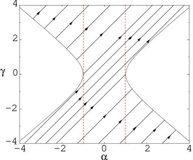
Figure 2: Phase-space trajectories in the $(\alpha,\gamma)$ plane for $\lambda=2$. Everywhere within the red dashed lines the universe will have a phantom equation of state.

Figure 3: Classification of phase-space trajectories in the $(\alpha,\gamma)$ plane for $\lambda=2$.

The evolution of the universe in each of the classes is

• : power-law contraction ($p=2/\lambda^{2}$) $~{}\rightarrow~{}$ bounce $~{}\rightarrow~{}$ power-law expansion ($p=2/\lambda^{2}$)

• : kinetic dominated contraction $~{}\rightarrow~{}$ bounce $~{}\rightarrow~{}$ power-law expansion ($p=2/\lambda^{2}$)

• : power-law contraction ($p=2/\lambda^{2}$) $~{}\rightarrow~{}$ bounce $~{}\rightarrow~{}$ kinetic dominated expansion

• : Big Bang $~{}\rightarrow~{}$ kinetic dominated expansion $~{}\rightarrow~{}$ power-law expansion ($p=2/\lambda^{2}$)

• : power-law contraction ($p=2/\lambda^{2}$) $~{}\rightarrow~{}$ kinetic dominated contraction $~{}\rightarrow~{}$ Big Crunch

For $\lambda^{2}>6$ the phase trajectories evolve as shown in Figure 4. The different classes of solution are shown schematically in Figure 5. The trajectories fall into only three classes in this case. The evolution of the universe in each of the classes is:

• : kinetic dominated contraction $~{}\rightarrow~{}$ bounce $~{}\rightarrow~{}$ kinetic dominated expansion

• : Big Bang $~{}\rightarrow~{}$ kinetic dominated expansion

• : kinetic dominated contraction $~{}\rightarrow~{}$ Big Crunch

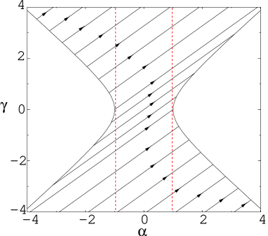
Figure 4: Phase-space trajectories in the $(\alpha,\gamma)$ plane for $\lambda=3$. Everywhere within the red dashed lines the universe will have a phantom equation of state.

Figure 5: Classification of phase-space trajectories in the $(\alpha,\gamma)$ plane for $\lambda=3$

The overall equation of state (8) of the system is

$$w=-1+\frac{2(\alpha^{2}-1)}{\gamma^{2}}\,.$$ (29)

In order to have phantom behaviour ($w<-1$) we therefore require $\alpha^{2}<1$.For $\lambda=0$, the trajectories are $\alpha=const$, and so are straight vertical lines in the $\gamma-\alpha$ phase plane. For $\lambda\neq 0$ no trajectory remains within the phantom region and we always have $w>-1$ at early times and late times.

In the second part of the paper we will study inhomogeneous perturbations about the solutions in class A, i.e., non-singular evolution for $\lambda^{2}<6$ where the ghost field is negligible at early and late times. From Eqs. (22) and (27) we find that this corresponds to solutions with integration constant

$$C^{2}<1-\frac{\lambda^{2}}{6}\,.$$ (30)

III Linear perturbations

The most general metric of a perturbed FRW universe can be written to first order

$$g_{\mu\nu}=a^{2}(\eta)\left(\begin{array}[]{cc}-(1+2\phi)&B_{|i}-S_{i}\\ B_{|j}-S_{j}&(1-2\psi)\gamma_{ij}+2E_{|ij}+F_{i|j}+F_{j|i}+h_{ij}\end{array}\right)\,.$$

The scalar quantity $\phi$ describes the perturbation in the lapse function, $\psi$ describes the perturbation of the intrinsic 3-curvature and the scalar shear is given by

$$\sigma=E^{\prime}-B\,.$$ (31)

We need to consider only the scalar and tensor parts ($h_{ij}$) of the metric perturbations, which remain decoupled to first-order. Vector perturbations ($S_{i}$ and $F_{i}$) can be eliminated by a gauge transformation when the energy-momentum tensor only comes from scalar fields MFB92 .

We can also express the perturbed fields in terms of their homogeneous background value plus an inhomogeneous perturbation

$$\varphi = \varphi_{0}+\delta\varphi\,,$$ (32)

$$\chi = \chi_{0}+\delta\chi\,.$$ (33)

Under a first-order time-shift, or temporal gauge transformation,

$$\tilde{\eta}=\eta+\xi^{0}\,,$$ (34)

the scalar metric perturbations transform as MFB92

$$\tilde{\phi} = \phi-h\xi^{0}-{\xi^{0}}^{\prime}\,,$$ (35)

$$\tilde{\psi} = \psi+h\xi^{0}\,,$$ (36)

$$\tilde{\sigma} = \sigma+\xi^{0}\,,$$ (37)

and the first-order field perturbations transform as

$$\tilde{\delta\varphi} = \delta\varphi-\varphi^{\prime}\xi^{0}\,,$$ (38)

$$\tilde{\delta\chi} = \delta\chi-\chi^{\prime}\xi^{0}\,.$$ (39)

The tensor metric perturbations, $h_{ij}$, are gauge-invariant.

The linearly perturbed Klein-Gordon equations for the two fields give the wave equations for the field perturbations:

$$\delta\varphi^{\prime\prime}+2h\delta\varphi^{\prime}-\nabla^{2}\delta\varphi+a^{2}V_{,\varphi\varphi}\delta\varphi+2a^{2}V_{,\varphi}\phi-\varphi_{0}^{\prime}\phi^{\prime}-\varphi_{0}^{\prime}(3\psi^{\prime}-\nabla^{2}\sigma) = 0\,,$$ (40)

$$\delta\chi^{\prime\prime}+2h\delta\chi^{\prime}-\nabla^{2}\delta\chi-\chi_{0}^{\prime}\phi^{\prime}-\chi_{0}^{\prime}(3\psi^{\prime}-\nabla^{2}\sigma) = 0\,.$$ (41)

Similarly the Einstein equations can be split into background and perturbed parts, yielding the background Eqs. (5) and (6), and to first-order

$$-3h(h\phi+\psi^{\prime})+\nabla^{2}[\psi+h\sigma] = -\frac{\kappa^{2}}{2}(\phi({\varphi_{0}^{\prime}}^{2}-{\chi_{0}^{\prime}}^{2})-\varphi_{0}^{\prime}\delta\varphi^{\prime}+\chi_{0}^{\prime}\delta\chi^{\prime}-a^{2}V_{,\varphi}\delta\varphi)\,,$$ (42)

$$h\phi+\psi^{\prime} = -\frac{\kappa^{2}}{2}(\chi_{0}^{\prime}\delta\chi-\varphi_{0}^{\prime}\delta\varphi)\,,$$ (43)

$$(2h^{\prime}+h^{2})\phi+h\phi^{\prime}+\psi^{\prime\prime}+2h\psi^{\prime} = \frac{\kappa^{2}}{2}\left[\right.\varphi_{0}^{\prime}\delta\varphi^{\prime}-\chi_{0}^{\prime}\delta\chi^{\prime}-\phi({\varphi_{0}^{\prime}}^{2}-{\chi_{0}^{\prime}}^{2})-a^{2}V_{,\varphi}\delta\varphi\left.\right]\,,$$ (44)

$$\sigma^{\prime}+2h\sigma+\psi-\phi = 0\,.$$ (45)

An arbitrary inhomogeneous perturbation can then be decomposed into a superposition of independent Fourier modes with comoving wavenumber $k$, such that $\nabla^{2}\delta\varphi=-k^{2}\delta\varphi$.

The gauge-transformation equations (35–39) show that the evolution equations contain an unphysical gauge mode, identified with the choice of constant-time hypersurfaces, as well as the physical degrees of freedom. To remove this ambiguity one can work with gauge-invariant variables, but there is no unique choice of gauge-invariant variables, such as, for example, the curvature perturbation.

To determine the initial vacuum fluctuations at early times in a collapsing phase and then follow these perturbations through the bounce phase we will solve the perturbations in two specific choices of gauge, each adapted to one phase of the evolution. Either gauge can be used to define different gauge-invariant variables MW1 . Because we have gauge-invariant definitions in each phase we can consistently follow the perturbations through from early to late times.

Ultimately we will present our final results in terms of the two most commonly used gauge-invariant curvature perturbations:

$${\cal{R}} = \psi+\frac{h(\varphi^{\prime}\delta\varphi-\chi^{\prime}\delta\chi)}{\varphi^{\prime 2}-\chi^{\prime 2}}\,,$$ (46)

$$\Phi = \psi+h\sigma\,.$$ (47)

Equation (46) is the natural generalisation of the usual comoving curvature perturbation for two scalar fields GBW ; Gordon to the case where one of them is a ghost field, while Eq. (47) is the curvature perturbation in the longitudinal gauge MFB92 , also called the Bardeen potential.

III.1 Uniform curvature gauge

In order to describe the early time behaviour close to the fixed point $B_{-}$ we will first work in the uniform curvature (or spatially flat) gauge in which the metric perturbation, $\psi$ vanishes. This is the gauge commonly used to describe vacuum fluctuations generated during inflation Sasaki ; LythStewart ; hwang .

From Eq. (36) we see that $\tilde{\psi}=0$ corresponds to a specific time-shift from an arbitrary gauge

$$\xi^{0}=-\frac{\psi}{h}\,,$$ (48)

This enables us to give a gauge-invariant definitions of the remaining metric perturbations MW1 and, in particular, the scalar field perturbations in the uniform-curvature gauge

$$\tilde{\delta\varphi}|_{\psi} \equiv \delta\varphi+\frac{\varphi^{\prime}}{h}\psi\,,$$ (49)

$$\tilde{\delta\chi}|_{\psi} \equiv \delta\chi+\frac{\chi^{\prime}}{h}\psi\,.$$ (50)

In the rest of this sub-section we will drop the tilde and $\psi$-subscript, but it should be remembered that all perturbations correspond to those in the uniform-curvature gauge.

Using Eqs.(42–45) to eliminate $\phi$ and $\psi$, the perturbed Klein-Gordon equations in the uniform-curvature gauge can be written as two coupled second-order equations for the field perturbations:

$${\delta\varphi^{\prime\prime}}-\nabla^{2}{\delta\varphi}+2h{\delta\varphi^{\prime}}+\left[a^{2}V_{,\varphi\varphi}+\kappa^{2}\varphi_{0}^{\prime}\left(\varphi_{0}^{\prime}(\frac{h^{\prime}}{h^{2}}-2)-2\frac{\varphi_{0}^{\prime\prime}}{h}\right)\right]{\delta\varphi} = \frac{\kappa^{2}\chi_{0}^{\prime}}{h}(\varphi_{0}^{\prime}\frac{h^{\prime}}{h}-\varphi_{0}^{\prime\prime}){\delta\chi}\,,$$ (51)

$${\delta\chi^{\prime\prime}}-\nabla^{2}{\delta\chi}+2h{\delta\chi^{\prime}}-\kappa^{2}\chi_{0}^{\prime 2}(2+\frac{h^{\prime}}{h^{2}}){\delta\chi} = \frac{\kappa^{2}\chi_{0}^{\prime}}{h}(\varphi_{0}^{\prime\prime}-\frac{h^{\prime}}{h}\varphi_{0}^{\prime}){\delta\varphi}\,.$$ (52)

These evolution equations in the uniform-curvature gauge have a simple form which is convenient for studying the evolution during monotonic expansion or collapse. In particular we will use this gauge to describe the initial quantum fluctuations during a collapse phase.

However these equations are not suitable for evolving the perturbations through a bounce. The evolution equations (51) and (52) contain singular coefficients as $h\to 0$. This is not surprising as from Eq. (48) we see that the uniform-curvature gauge is itself ill-defined at a bounce as $h\to 0$. Instead, we have to find another gauge which remains well-defined at the bounce in order to evolve the initial vacuum perturbations through to an expanding phase.

III.2 Uniform $\chi$-field gauge

Analogously to the background solutions where we used the $\chi$-field as a useful time coordinate to study evolution through the bounce, we will use the uniform-$\chi$ gauge to follow linear perturbations through the bounce.

From Eq. (39) we see that to set $\tilde{\delta\chi}=0$ we must choose

$$\xi^{0}=\frac{\delta\chi}{\chi^{\prime}}\,.$$ (53)

The remaining $\varphi$-field perturbation in the uniform-$\chi$ gauge has the gauge invariant definition

$$\tilde{\delta\varphi}|_{\chi}\equiv\delta\varphi-\frac{\varphi^{\prime}}{\chi^{\prime}}\delta\chi\,.$$ (54)

The scalar metric perturbations $\phi$, $\psi$ and $\sigma$ in the uniform-$\chi$ gauge also have gauge-invariant definitions. In particular the curvature perturbation on uniform-$\chi$ hypersurfaces is given by

$$\tilde{\psi}|_{\chi}\equiv\psi+\frac{h}{\chi^{\prime}}\delta\chi\,.$$ (55)

In the rest of this sub-section we will drop the tilde and $\chi$-subscript, but it should be remembered that all perturbations correspond to those in the uniform-$\chi$ gauge.

The perturbed Klein-Gordon and Einstein equations (40–45), then give us the four evolution equations for the four perturbation variables $\delta\varphi,~{}\psi,~{}\phi$ and $\sigma$ in the uniform $\chi$-field gauge

$$\kappa\delta\varphi_{,qq}+\frac{6k^{2}}{\kappa^{2}{\chi^{\prime}}^{2}}\kappa\delta\varphi+3\beta^{2}\lambda^{2}\kappa\delta\varphi-6\lambda\beta^{2}\phi = 0\,,$$ (56)

$$\psi_{,qq}-\frac{3\alpha}{\sqrt{6}}\kappa\delta\varphi_{,q}-\frac{3\lambda\beta^{2}}{2}\kappa\delta\varphi+\gamma\phi_{,q}+3\beta^{2}\phi = 0\,,$$ (57)

$$\phi_{,q}+3\psi_{,q}+\frac{6k^{2}}{\kappa^{2}{\chi^{\prime}}^{2}}s = 0\,,$$ (58)

$$s_{,q}+4\gamma s+\psi-\phi = 0\,,$$ (59)

plus two constraint equations

$$\gamma\phi+\psi_{,q}-\frac{\sqrt{6}\alpha}{2}\kappa\delta\varphi = 0\,,$$ (60)

$$(\alpha^{2}-1)\phi-\frac{\alpha}{\sqrt{6}}\kappa\delta\varphi_{,q}+(\frac{\lambda\beta^{2}}{2}-\frac{3\alpha\gamma}{\sqrt{6}})\kappa\delta\varphi-\frac{2k^{2}}{\kappa^{2}{\chi^{\prime}}^{2}}(\psi+\gamma s) = 0\,.$$ (61)

Here we have (as for the background evolution) we have written time derivatives with respect to the dimensionless, and monotonic, variable $q$ defined in Eq. (23). We have written background quantities in terms of the dimensionless variables $\alpha$, $\beta$ and $\gamma$ defined in Eqs. (19–21).

We have rescaled the shear perturbation variable $\sigma$ in terms of

$$s\equiv\frac{h}{\gamma}\sigma\,,$$ (62)

so that all gradient terms enter through terms of order $(k/\kappa\chi^{\prime})^{2}$ which is the square of $\gamma$ times the ratio of the Hubble length to the wavelength. Thus we can obtain solutions order-by-order in terms of $(k/\kappa\chi^{\prime})^{2}$ to define a long-wavelength limit. Although the Hubble length diverges at the bounce we have from Eq. (7) that $(k/\kappa\chi^{\prime})^{2}\propto a^{4}$. This remains finite and actually reaches a minimum at the bounce. Thus we find that the long-wavelength solution, neglecting terms of order $(k/\kappa\chi^{\prime})^{2}$ is an excellent solution close to the bounce for scales of interest.

In principle we could use the constraint equations (60) and (61) to eliminate $\phi$ and $s$ respectively and leave two second-order equations for $\delta\varphi$ and $\psi$, similar to what was done for the uniform curvature gauge perturbations in the preceding subsection. However as $\gamma\to 0$ approaching a bounce this approach would be very sensitive to any small numerical error. We will not eliminate $\phi$ and $s$ and instead will use their first-order evolution equations to evolve them numerically through the bounce. The constraint equations (60) and (61) then provide a useful consistency check for our numerical integrations. A similar argument in favour of using coupled first-order equations to study perturbations through a bounce was recently given by Cartier Cartier .

III.3 Tensor perturbations

The tensor part of the perturbed metric, $h_{ij}$, is transverse and trace-free and is invariant under gauge transformations. We expand $h_{ij}$ in plane-waves

$$h_{ij}({\bf x},\eta)=(2\pi)^{-3}\int d^{3}{\bf k}\sum_{p=\times,+}\ \delta g^{p}_{\bf k}(\eta)\,\epsilon^{p}_{ij}({\bf k,x})\,,$$ (63)

where $\epsilon^{p}_{ij}$ is the polarisation tensor and $p=\times,~{}+$ represents the two independent polarisation states. $\delta g^{\times,+}_{\bf{k}}$ is the scalar amplitude of each state for wave-mode $\bf{k}$. For both polarisation states this scalar amplitude obeys the simple wave equation for a free scalar field in an FRW spacetime,

$$\delta g^{\prime\prime}+2h\delta g^{\prime}+k^{2}\delta g=0\,,$$ (64)

where $k^{2}={\bf k.k}$. Here and from now on the subscript $k$ and the superscript $\times,+$ are assumed for $\delta g$.

Under transformation to derivatives with respect to our monotonic time variable $q$ defined in Eq. (23), the tensor evolution Eq. (64) becomes

$$\delta g_{,qq}+\frac{6k^{2}}{\kappa^{2}{\chi^{\prime}}^{2}}\delta g=0\,.$$ (65)

This is the form of the equation that we use to evolve the tensor perturbations numerically through the bounce.

IV Vacuum fluctuations

IV.1 Early-time behaviour in uniform-curvature gauge

For any power-law solution described by a critical point in the dimensionless phase-space we have $\varphi^{\prime}\propto h$ and the right-hand-sides of Eqs. (51) and (52) vanish. Thus the field perturbations $\delta\varphi$ and $\delta\chi$ in the uniform-curvature gauge decouple in the early-time limit where the background solution is described by Eq. (17). In this case the evolution equations for the field perturbations can be written very simply in terms of the canonical Sasaki/Mukhanov variables MFB92

$$u_{\varphi} = a\delta\varphi\,,$$ (66)

$$u_{\chi} = a\delta\chi\,,$$ (67)

For each Fourier mode with comoving wavenumber $k$, Eqs. (51) and (52) can then be written as

$$u_{i}^{\prime\prime}+\left(k^{2}-\frac{a^{\prime\prime}}{a}\right)u_{i}=0\,,$$ (68)

where $i=\varphi,\chi$. The evolution equation for the tensor perturbations Eq. (64) can be written in exactly the same form, where

$$u_{g}=\frac{a\delta g}{2\kappa}\,.$$ (69)

For power law expansion or collapse described by Eq. (17) the equation (68) has the general solution LythStewart

$$u=\sqrt{|k\eta|}[u_{+}H_{(|\nu|)}^{(1)}(|k\eta|)+u_{-}H_{(|\nu|)}^{(2)}(|k\eta|)]\,,$$ (70)

where the index

$$\nu\equiv\frac{3}{2}+\frac{1}{p-1}\,.$$ (71)

Although the scalar fields $\varphi$ and $\chi$ are real scalar fields, we have chosen to Fourier expand the perturbations in terms of complex Fourier modes $\propto e^{\pm ikx}$. Thus we work with the complex modes functions (70) which must obey the condition $u(-k)=u^{*}(k)$.

At early times ($\eta\ll-k^{-1}$) we have free oscillations $u\propto e^{\pm ik\eta}$. The simplest assumption is that the perturbation variables, $u_{1,2}$, start in the flat space-time vacuum state with only positive frequency modes, satisfying the normalisation condition

$$u^{\prime}u^{*}-{u^{*}}^{\prime}u=i\,.$$ (72)

Thus at early times ($k\eta\to-\infty$) we require

$$u\to\frac{1}{(2k)^{\frac{1}{2}}}e^{-ik\eta}\,.$$ (73)

Using the vacuum solution (73) at early times to set the initial conditions for the general solution (70) yields

$$u=\frac{\sqrt{\pi}}{2}\frac{e^{i(|\nu|+\frac{1}{2})\frac{\pi}{2}}}{k^{\frac{1}{2}}}|k\eta|^{\frac{1}{2}}H^{(1)}_{|\nu|}(|k\eta|)\,.$$ (74)

We use this analytic vacuum solution for the three perturbation variables to set up the initial conditions for the perturbations in our numerical code. We start the code far away from the bounce when we are still well within the power-law regime ($p\simeq 2/\lambda^{2}$). However, as we saw in Section II, this power-law solution is unstable and as the universe collapses the evolution will eventually diverge away from the critical point.

IV.1.1 Initial power spectra

$\delta\varphi$, $\delta\chi$ and $\delta g$ are independent Gaussian random fields whose distribution will be completely determined by the power spectra, defined for a scalar $\delta x$ as

$$\mathcal{P}_{x}\equiv\frac{k^{3}|\delta x|^{2}}{2\pi^{2}}\,.$$ (75)

The tilt of the spectrum is defined by

$$\Delta n_{x}\equiv\frac{d\ln(\mathcal{P}_{x})}{d\ln(k)}\,,$$ (76)

so that $\Delta n_{x}=0$ for a scale-invariant spectrum. Note that the conventional spectral index for scalar metric perturbations is given by $n=1+\Delta n_{x}$.

As $\delta\varphi$ and $\delta\chi$ are independent fields in the initial power-law regime, we can find the power spectrum for any quantity by evolving separately different modes corresponding to an initial perturbation in $\varphi$ or $\chi$. The power due to each mode can be summed to obtain the final spectrum. $\varphi$-modes correspond to initial vacuum perturbations of the $\varphi$-field on the uniform curvature hypersurface with the $\chi$ perturbation (and its derivative) initially zero on this hypersurface. $\chi$-modes correspond to the opposite situation, where there is an initial perturbation of the $\chi$-field but no perturbation of the $\varphi$ field (or its derivative) on the uniform curvature hypersurface.

Any complex variable can be split into two parts whose phase differs by 90^∘, which typically might be real and imaginary parts. We find it convenient to split the Hankel function, $H_{|\nu|}^{(1)}$, found in our general solution for $u$, Eq. (74), into real Bessel functions of the first and second kind:

$$H_{|\nu|}^{(1)}(|k\eta|)=J_{|\nu|}(|k\eta|)+iY_{|\nu|}(|k\eta|)\,.$$ (77)

We will thus refer to these as the $J$ and $Y$ modes. From the definition of the power spectrum Eq. (75) it can then be seen that

$$\mathcal{P}_{x}=\mathcal{P}_{x_{J}}+\mathcal{P}_{x_{Y}}$$ (78)

Thus, the $J$ and $Y$ parts can be evolved separately to determine the total power spectrum. This gives us four independent ’modes’ or sets of initial conditions ($\varphi_{J}$, $\varphi_{Y}$, $\chi_{J}$, and $\chi_{Y}$) for which we present our numerical results.

The Bessel functions of first and second kind describe regular and singular solutions on large scales ($|k\eta|\rightarrow 0$) behaving as

$$J_{|\nu|}(|k\eta|) \rightarrow \frac{1}{\Gamma(|\nu|+1)}\left(\frac{|k\eta|}{2}\right)^{|\nu|}\,,$$ (79)

$$Y_{|\nu|}(|k\eta|) \rightarrow -\frac{\Gamma(|\nu|)}{\pi}\left(\frac{|k\eta|}{2}\right)^{-|\nu|}\,.$$ (80)

Thus, from Eqs (74), we see that the power spectrum from vacuum fluctuations during collapse on large scales yields

$$\mathcal{P}_{u}=C_{J}^{2}(|\nu|)k^{2}|k\eta|^{1+2|\nu|}+C_{Y}^{2}(|\nu|)k^{2}|k\eta|^{1-2|\nu|}\,,$$ (81)

where

$$C_{J}(|\nu|) \equiv \frac{1}{2^{|\nu|+\frac{3}{2}}\sqrt{\pi}\Gamma(|\nu|+1)}\,,$$ (82)

$$C_{Y}(|\nu|) \equiv \frac{2^{|\nu|-\frac{3}{2}}\Gamma(|\nu|)}{\pi^{\frac{3}{2}}}\,.$$ (83)

The spectral tilts for each term in the spectrum (81) are then LythStewart ; Wands99

$$\Delta n_{u_{J}} = 3+2|\nu|\,,$$ (84)

$$\Delta n_{u_{Y}} = 3-2|\nu|\,.$$ (85)

In a contracting universe the second $Y$-term in Eq. (81) should quickly dominate on super-Hubble scales as $k\eta\to 0$. However, we will evolve both modes numerically to see whether this will remains true through the bounce or whether the less dominant mode in the collapsing phase will come to dominate in the expanding phase.

We will present detailed numerical solutions for interesting physical choices of the scalar field slope, $\lambda$, and hence power-law $p$ in the collapse phase that give simple analytic solutions for the perturbations during the initial power-law collapse phase.

IV.1.2 $\lambda=2$: Power-law solution with $p=1/2$

Taking $\lambda=2$ means that the scale factor will follow the same evolution as a radiation dominated universe with $w=1/3$ and $p=1/2$ at the critical points $B_{\pm}$.

The Hankel function index in Eq. (71) is $\nu=-1/2$ and for this special case the first Hankel function has the simple form

$$H^{(1)}_{\frac{1}{2}}(z)=\sqrt{\frac{2}{\pi z}}(\sin(z)-i\cos(z))\,.$$ (86)

and the vacuum solutions (74) become

$$u=\frac{1}{(2k)^{\frac{1}{2}}}(\cos(|k\eta|)+i\sin(|k\eta|))$$ (87)

In this case the $Y$-part of the solution corresponds to the real part of the solution which will dominate in the collapsing universe as $k\eta\to 0$.

The spectral tilts of the $Y$ and $J$ parts of $u$ are then given by

$$\Delta n_{u_{Y}} = 2\,,$$ (88)

$$\Delta n_{u_{J}} = 4\,.$$ (89)

Both modes have steep blue tilts.

IV.1.3 $\lambda=\sqrt{3}$: Power-law solution with $p=2/3$

Taking $\lambda=\sqrt{3}$ means that the scale factor will follow the same evolution as a matter dominated universe at the critical points $B_{\pm}$, with $w=0$ and $p=2/3$.

The Hankel function index in Eq. (71) is $\nu=-3/2$ and for this special case the first Hankel function has the simple form

$$H^{(1)}_{3/2}(z)=-\sqrt{\frac{2}{\pi z}}\left(1-\frac{1}{iz}\right)(\cos(z)+i\sin(z))\,.$$ (90)

and the solution for $u$ will be

$$u=\frac{1}{(2k)^{\frac{1}{2}}}\left[\left(\cos(|k\eta|)-\frac{\sin(|k\eta|)}{|k\eta|}\right)+i\left(\sin(|k\eta|)+\frac{\cos(|k\eta|)}{|k\eta|}\right)\right]$$ (91)

This is the same mode function as is found for a vacuum fluctuations of a massless field in de Sitter inflation Wands99 . Here the $Y$-mode is the imaginary part of the solution will dominate in a collapsing universe as $k\eta\to 0$.

The spectral tilts of the $Y$ and $J$ parts of the field fluctuations on large scale are

$$\Delta n_{u_{Y}} = 0\,,$$ (92)

$$\Delta n_{u_{J}} = 2\,.$$ (93)

The $J$ part has a steep blue tilt, but the $Y$ part, which dominates as $k\eta\to 0$, has a scale-invariant spectrum Starobinsky ; Wands99 ; FB .

IV.2 Numerical evolution through the bounce

The initial conditions for the background variables are set so that the evolution follows a trajectory in the phase-plane that lies within region A, as defined in section(II.2). Thus the evolution starts close to the critical point $B_{-}$ where it follows a power-law collapse solution. It eventually diverges away from this critical point as the universe collapses and the (negative) kinetic energy of the $\chi$ field grows than that of the $\varphi$ field. The scale factor smoothly evolves through the bounce and finally moves towards the critical point $B_{+}$ in the expanding phase, where once again the model approaches a power-law solution with $p=2/\lambda^{2}$.

We use Eqs. (56-59) to evolve the scalar perturbations in the uniform $\chi$-field gauge through the bounce using $q$ as our monotonically increasing time variable. This requires initial conditions for $\delta\varphi,~{}\delta\varphi_{,q},~{}\psi,~{}\psi_{,q},~{}\phi$ and $s$ in each mode. The first four initial conditions are found from our analytical solutions in section(IV.1). However, as these solutions are found in the uniform curvature gauge it is necessary to transform them to the uniform $\chi$-field gauge. It is also necessary to change the time variable from $\eta$ to $q$. The appropriate gauge transformation (53) gives

$$\delta\varphi|_{\chi} = \delta\varphi|_{\psi}-\alpha\delta\chi|_{\psi}\,,$$ (94)

$$\delta\varphi_{,q}|_{\chi} = -\frac{\lambda\sqrt{6}\beta^{2}}{2}\delta\chi|_{\psi}+\frac{\sqrt{6}}{\kappa\chi^{\prime}}(\delta\varphi^{\prime}|_{\psi}-\alpha\delta\chi^{\prime}|_{\psi})\,,$$ (95)

$$\psi|_{\chi} = \frac{\kappa\gamma}{\sqrt{6}}\delta\chi|_{\psi}\,,$$ (96)

$$\psi_{,q}|_{\chi} = \frac{3\kappa\beta^{2}}{\sqrt{6}}\delta\chi|_{\psi}+\frac{\gamma}{\chi^{\prime}}\delta\chi^{\prime}|_{\psi}\,.$$ (97)

The other two initial conditions required, for $\phi$ and $s$, are found from the constraints (60,61). Thereafter the constraint equations serve as a consistency check of our numerical solutions.

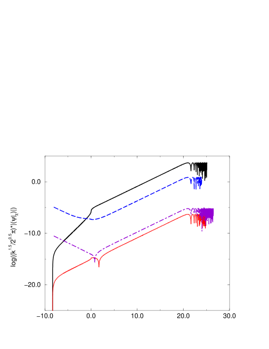
Figure 6: Evolution of $\psi|_{\chi}$ shown as a function of expansion, $N=\pm\ln(a/a_{0})$, for bounce solution with $\lambda=2$ model for each of the four independent modes: $\varphi_{Y}$ (black solid line), $\varphi_{J}$ (red dotted line), $\chi_{Y}$ (blue dashed line), and $\chi_{J}$ (purple dot-dashed line).

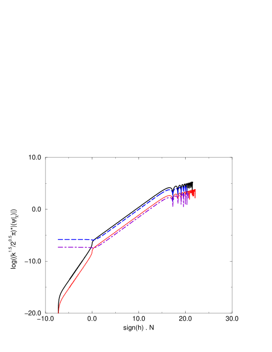
Figure 9: Evolution of $\psi|_{\chi}$ shown as a function of expansion, $N=\pm\ln(a/a_{0})$, for bounce solution with $\lambda=\sqrt{3}$ model for each of the four independent modes: $\varphi_{Y}$ (black solid line), $\varphi_{J}$ (red dotted line), $\chi_{Y}$ (blue dashed line), and $\chi_{J}$ (purple dot-dashed line).

The dimensionless metric perturbations $\psi$ and $\phi$ remain small in the uniform $\chi$-field gauge and well-behaved through the bounce. Typical numerical solutions for the curvature perturbation $\psi$ is shown in Figure 6 for $\lambda=2$ and Figure 9 for $\lambda=\sqrt{3}$. The perturbed lapse function $\phi$ closely follows the curvature perturbation on large scales, where we find $\phi+3\psi\simeq$constant, as expected from Eq. (58).

The shear potential $\sigma$ does grow rapidly in the collapse phase, reflecting the instability with respect to shear of the power-law solution. From Eq. (44) we see that in any gauge where $\phi$ and $\psi$ remain small, we find $\sigma\propto a^{-2}$ as the collapse proceeds. However the shear only enters the evolution equation (58) for $\phi$ through its spatial divergence and this term remains small as the bounce is approached. We have checked that the magnitude of the shear term in, for example, the energy constraint equation (61), is always much smaller than, for instance, the energy density of either of the scalar fields. Note that the total density, and hence the isotropic expansion rate, goes to zero at the bounce, so the anisotropic shear perturbation cannot be smaller than the isotropic expansion/collapse at this point but it is always small relative to the largest terms in the equation so we believe our perturbative analysis is justified.

All the $k$-dependent terms in the evolution equations (56–59) in the uniform-$\chi$ gauge become small as we approach the bounce and we find that the $k=0$ solution is an excellent approximation through the bounce for modes which leave the Hubble scale well before the bounce ($k\ll(aH)_{\rm max}$). Note the difference with models of a classical bounce in closed FRW geometries, where finite scale effects may be significant as modes re-enter the horizon during the bounce MP .

At late times, in the expanding phase after the bounce, the curvature perturbation in the uniform $\chi$-field gauge gradually grows and eventually may become larger than one. This is because $\chi^{\prime}\to 0$ as we asymptotically approach the power-law solution once again and the gauge shift (53) becomes large. Thus at late times in the expanding universe we should transform back to some well-behaved gauge, such as the longitudinal or uniform-curvature gauges, where the metric perturbations remain small. Nonetheless the uniform $\chi$-field gauge does the job of evolving the initial vacuum fluctuations from the collapse phase smoothly through the bounce into an expanding phase where the large-scale behaviour is unambiguous.

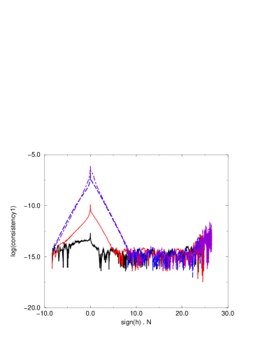
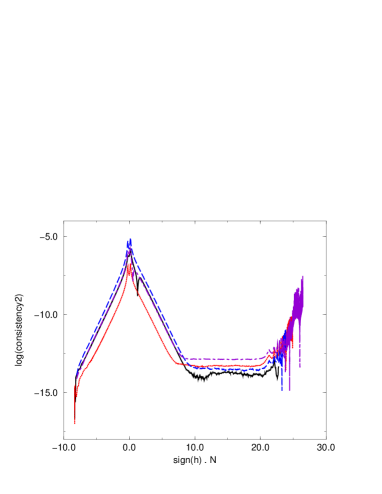
Figure 14: The violation of constraint equations (60) and (61) shown as a function of expansion, $N=\pm\ln(a)$, for a bounce solution in the $\lambda=2$ model for each of the four independent scalar modes: $\varphi_{Y}$ (black solid line), $\varphi_{J}$ (red dotted line), $\chi_{Y}$ (blue dashed line), $\chi_{J}$ (purple dot-dashed line). The $y$-axis of the left hand graph shows the logarithm of the absolute value of the left hand side of Eq. (60) divided by the sum of the absolute values of each term in the equation. The $y$-axis of the right hand graph shows the same thing for Eq. (61).

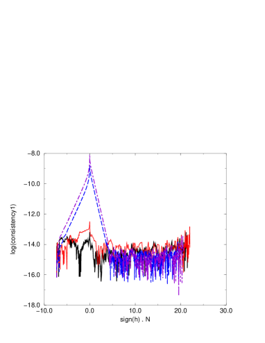
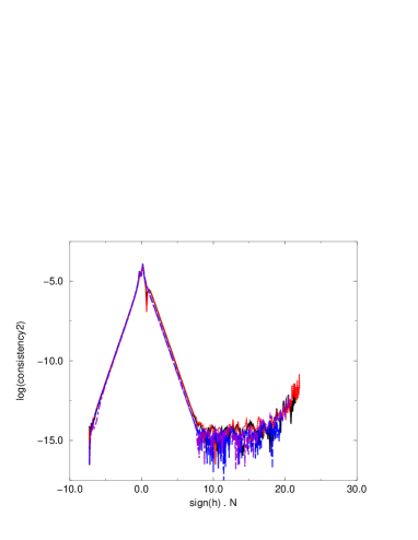
Figure 15: The violation of constraint equations (60) and (61) shown as a function of expansion, $N=\pm\ln(a)$, for a bounce solution in the $\lambda=\sqrt{3}$ model for each of the four independent scalar modes: $\varphi_{Y}$ (black solid line), $\varphi_{J}$ (red dotted line), $\chi_{Y}$ (blue dashed line), $\chi_{J}$ (purple dot-dashed line). The $y$-axis of the left hand graph shows the logarithm of the absolute value of the left hand side of Eq. (60) divided by the sum of the absolute values of each term in the equation. The $y$-axis of the right hand graph shows the same thing for Eq. (61).

The constraint equations (60) and (61) are satisfied to one part in ten thousand or better for all our numerical runs (see Figures 14 and 15).

V Results for gauge-invariant variables

In order to compare our results with previous discussions of the expected evolution of perturbations through a cosmological bounce, we reconstruct the gauge-invariant variables $\cal{R}$ and $\Phi$ defined in Eqs. (46) and (47) from the variables evolved numerically in the uniform-$\chi$ gauge.

For our two chosen values of $\lambda=2$ and $\lambda=\sqrt{3}$, we find the power spectra of these two gauge-invariant variables for each mode when the background is asymptotically evolving as the power law collapse and expansion. We compare the spectral tilts of the power spectra before and after the bounce and we see whether the mode dominant before the bounce remains so after it.

Tensor perturbations $\delta g$ are automatically gauge-invariant and provide an interesting comparison with the scalar metric perturbations. Tensors also turn out to place an important constraint on models producing a scale-invariant spectrum of large-scale perturbations.

V.1 Comoving curvature perturbation

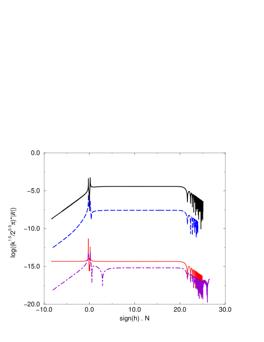
Figure 7: Comoving curvature perturbation $\cal{R}$ calculated from numerical solution for each of the four modes shown in Figure 6.

Typical evolution of the comoving curvature perturbation, ${\cal R}$ [defined in Eq. (46)], through the bounce is shown in Figures 7 for $\lambda=2$ and 10 for $\lambda=\sqrt{3}$. The four lines correspond to the four modes identified in section IV.1. ${\cal R}$ only remains constant on large scales for the $\varphi_{J}$ mode when $\lambda=2$, when this corresponds to an adiabatic perturbation of the power-law solution. All the other modes represent non-adiabatic perturbations about the initial power-law solution on large scales and have non-constant ${\cal R}$. In particular the dominant mode, $\varphi_{Y}$, describes non-adiabatic perturbations of the $\varphi$ field. Perturbations in the $\chi$ field are always sub-dominant in terms of their contribution to the comoving curvature perturbation.

During the bounce phase we see two singular points in the evolution of ${\cal R}$. This occurs whenever the total kinetic energy vanishes, $\varphi^{\prime 2}-\chi^{\prime 2}=0$ (corresponding to $\alpha^{2}=1$ in the phase-plane), as can be seen from the definition of ${\cal R}$ given in Eq. (46). At these points the total four-velocity of the two-field system is momentarily ill-defined. This makes the comoving gauge unsuitable for evolving the perturbations close to the bounce. We emphasise though that we can nonetheless trust the evolution of ${\cal R}$ shown in Figures (7) and (10) because here the comoving curvature has been constructed from perturbations in the uniform-$\chi$ gauge which remain well-behaved throughout the bounce, i.e., we do not require that the perturbations are necessarily small or well-defined in any other gauge.

After the bounce the comoving curvature perturbation rapidly settles down to a constant value for all modes on all super-Hubble scales, representing the resultant adiabatic curvature perturbation on large scales. Thus all the modes contribute a finite amplitude to the large-scale curvature perturbation in the expanding phase, and this is approximately equal to the amplitude of the comoving curvature perturbation at the end of the collapse phase (but not in general the amplitude at Hubble-crossing during collapse). The dominant mode at late times is the $\varphi_{Y}$ mode that also dominates the comoving curvature perturbation in the collapse phase.

Finally the perturbations “re-enter the horizon” in the expanding universe and oscillate for $k>aH$.

V.2 Bardeen potential

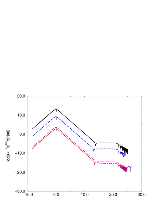
Figure 8: Bardeen metric potential $\Phi$ calculated from numerical solution for each of the four modes shown in Figure 6.

The typical evolution of the Bardeen potential, $\Phi$ defined in Eq. (47), which describes the curvature perturbation in the longitudinal gauge, is shown in Figures 8 for $\lambda=2$ and 11 for $\lambda=\sqrt{3}$.

All modes show the same rapid growth of $\Phi$ during the collapse phase. We can interpret this as being due to the rapid growth of the shear in the uniform-$\chi$ gauge, $\sigma|_{\chi}\propto a^{-2}$, while the curvature perturbation $\psi|_{\chi}$ remains small. According to the definition of $\Phi$ in Eq. (47) this yields a large curvature perturbation in the longitudinal gauge

$$\Phi\propto\frac{h}{a^{2}}\,.$$ (98)

Our numerical evolution for $\lambda=2$ and $\lambda=\sqrt{3}$ during the power-law collapse phase confirms this, yielding $\Phi\propto|\eta|^{-3}$ and $\Phi\propto|\eta|^{-5}$ respectively.

Thus the curvature perturbation in the longitudinal gauge becomes large in a collapse phase meaning that this gauge too may not be reliable gauge for performing a perturbative calculation through a cosmological bounce. Once again though we emphasise that our calculations of the Bardeen potential are reliable as we reconstruct the Bardeen potential from perturbative calculations in the uniform-$\chi$ gauge which remain small through the bounce.

After the bounce the dominant modes contributing to the Bardeen potential, $\varphi_{Y}$ and $\chi_{Y}$, remain dominated by the shear, $\sigma|_{\chi}$, which now decays in the expanding phase. Eventually the Bardeen potential settles down to a constant value on super-Hubble scales, before finally oscillating after re-entering the Hubble scale. For $\lambda=\sqrt{3}$ the sub-dominant modes, $\varphi_{J}$ and $\chi_{J}$, have much smaller shear (indeed $\Phi$ stays small for these modes right up until the bounce) and these modes rapidly settle down to a constant value soon after the bounce, but this final amplitude is smaller than that due to the dominant $\varphi_{Y}$ and $\chi_{Y}$ modes.

In summary we find that the amplitudes of the Bardeen potential during collapse are not a good predictor of the amplitude of the eventual adiabatic curvature perturbation on large scales after the bounce, even though it becomes much larger than the comoving curvature perturbation during the collapse. It is the growth of the shear that dominates the behaviour of $\Phi$ during the collapse and this shear then decays in the expanding phase. Only once the shear has decayed, sometime after the bounce, does $\Phi$ settle down to a constant value on super-Hubble scales in the expanding era.

For the case of $\lambda=2$ corresponding to a radiation-like equation of state $w=1/3$, we find that once the Bardeen potential has settled down to a constant value on super-Hubble scales, we have $\Phi=(2/3){\cal R}$. Similarly for $\lambda=\sqrt{3}$, corresponding to an equation of state $w=0$, we find $\Phi=(3/5){\cal R}$, as expected for the growing mode of adiabatic density perturbations on large scales.

V.3 Spectral tilts

V.3.1 $\lambda=2$: Asymptotic power-law solution with $p=1/2$

Table 1 shows the initial spectral tilts of the power spectra of $\cal{R}$ and $\Phi$, during power-law collapse with $\lambda=2$. All the modes of $\cal R$ have a blue spectrum, but the dominant mode of $\Phi$ has a red spectrum. Table 1 also shows the spectral tilts of the super-Hubble power spectra of $\cal{R}$ and $\Phi$ when they have settled to constant values after the bounce. The tilts of the spectra of $\cal R$ for each mode remain the same after the bounce as they were initially. The spectral tilt of $\Phi$ for every mode however becomes the same as that for the corresponding $\cal R$ spectra

$$\Delta n_{\Phi out}=\Delta n_{\Phi in}+4=\Delta n_{\cal R}\,.$$ (99)

Our model with $\lambda=2$ is very similar to the bounce model studied in Ref. PPN , but our results are strikingly different. The authors in that paper considered a radiation fluid which shows the same initial red spectrum for $\Phi$. But they found that the final spectrum for $\Phi$ retained the same red spectrum for $\Phi$. There are subtle differences between a radiation fluid and a $\lambda=2$ scalar field. In particular the bounce must be symmetrical with perfect fluids, whereas our bounce is only symmetrical for $C=0$ and our scalar field supports non-adiabatic pressure perturbations. But the main difference may come from the fact that a second-order evolution equation for $\Phi$ was used to follow the evolution of the metric perturbations in Ref. PPN . Perturbations in $\Phi$ become large and we have instead followed the evolution of perturbations in a gauge which remains well-behaved and then reconstructed the value of $\Phi$. We have not used the constraint equations to eliminate variables and have instead kept used these as a consistency check of our numerical integration.

mode	$\Delta n_{\cal{R}_{\rm in}}$	$\Delta n_{\Phi_{\rm in}}$	$\Delta n_{\cal{R}_{\rm out}}$	$\Delta n_{\Phi_{\rm out}}$
$\varphi_{Y}$	2	-2	2	2
$\varphi_{J}$	4	0	4	4
$\chi_{Y}$	2	-2	2	2
$\chi_{J}$	4	0	4	4

Table 1: Initial spectral tilts for different modes during collapse and final tilts after bounce for model with $\lambda=2$.

V.3.2 $\lambda=\sqrt{3}$: Asymptotic power-law solution with $p=2/3$

Table 2 shows the initial spectral tilts of the super-horizon power spectra of $\cal{R}$ and $\Phi$, during power-law collapse. The dominant mode of $\cal R$ has a scale-invariant spectrum Wands99 ; FB , whereas the spectrum of the dominant mode of $\Phi$ is red. Table 2 also shows the spectral tilts of $\cal{R}$ and $\Phi$ when they have settled to constant values on super-Hubble scales after the bounce. As for $\lambda=2$, the tilts of the spectra of $\cal R$ for each mode remain the same after the bounce as they were initially. In particular the dominant $\cal R$ mode retains its scale-invariant spectrum. The spectra of $\Phi$ again become the same as ${\cal R}$ after the bounce on large scales

$$\Delta n_{\Phi out}=\Delta n_{\Phi in}+4=\Delta n_{\cal R}\,.$$ (100)

Thus we have shown that a power-law collapse phase with $p=2/3$ can yield a scale-invariant spectrum of curvature perturbations on super-Hubble scales in the subsequent expanding phase.

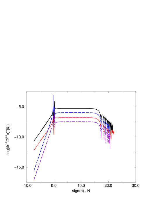
Figure 10: Comoving curvature perturbation $\cal{R}$ calculated from numerical solution for each of the four modes shown in Figure 9.

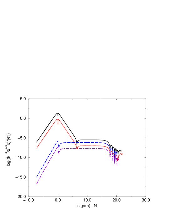
Figure 11: Bardeen metric potential $\Phi$ calculated from numerical solution for each of the four modes shown in Figure 9.

mode	$\Delta n_{\cal{R}_{\rm in}}$	$\Delta n_{\Phi_{\rm in}}$	$\Delta n_{\cal{R}_{\rm out}}$	$\Delta n_{\Phi_{\rm out}}$
$\varphi_{Y}$	0	-4	0	0
$\varphi_{J}$	2	-2	2	2
$\chi_{Y}$	0	-4	0	0
$\chi_{J}$	2	-2	2	2

Table 2: Initial spectral tilts of different modes during collapse and final tilts after bounce for model with $\lambda=\sqrt{3}$.

V.4 Tensor perturbations

The smooth evolution through the bounce of the amplitude of the tensor metric perturbations is shown in Figure 12. Tensor perturbations grow rapidly during the collapse phase but then rapidly settle down to a constant value after the bounce.

The spectral index of the tensor perturbations is the same as that of the comoving curvature perturbation ${\cal R}$ during collapse and, like the comoving curvature perturbation, the spectral index is unaffected by the bounce.

During power-law collapse there is a simple relation between the amplitude of tensor perturbations and the comoving curvature perturbation:

$$\left(\frac{{\cal P}_{g}}{{\cal P}_{\cal R}}\right)_{\rm collapse}=8\kappa^{2}\left(\frac{\varphi^{\prime}}{h}\right)^{2}\,.$$ (101)

For collapse solutions described by point $B$, we have, from Eqs. (16) and (17),

$$\left(\frac{{\cal P}_{g}}{{\cal P}_{\cal R}}\right)_{\rm collapse}=\frac{16}{p}\,.$$ (102)

In the model with $\lambda=\sqrt{3}$ which yields a scale-invariant spectrum of both scalar and tensor perturbations, this tensor-scalar ratio is $24$ during collapse.

However both the comoving curvature perturbation and tensor perturbation receive a scale-independent amplification during the bounce. This amplification is dependent upon the details of the bounce, and in particular the parameter $C$ defined in Eq. (27) which identifies the phase-space trajectory. We show in Figure 13 the resulting tensor-scalar ratio after the bounce. The tensor-scalar ratio is maximised for a symmetric bounce, $C=0$, which leaves the tensor-scalar ratio (102) unchanged. For an asymmetric bounce, the scalars are more strongly amplified than the tensor modes and the tesnor-scalar ratio becomes small for the most asymmetric bounces.

Observations require that the primordial tensor-scalar ratio is less than 0.81 WMAP . We see that this places a severe constraint on the allowed parameter $|C|>0.67$, given that from Eq. (30) we require $|C|<0.71$ for the collapse phase to end in a non-singular bounce. Although we have a tight constraint in our particular bounce model, it is not clear how problematic this might be in the more general case as asymmetry through the bounce can decrease the tensor-scalar ratio.

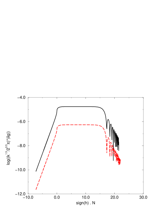
Figure 12: Evolution of $\delta g$ shown as a function of expansion, $N=\pm\ln(a)$, for a bounce solution in the $\lambda=\sqrt{3}$ model for each of the two independent tensor modes: $g_{Y}$ (solid black line) and $g_{J}$ (dashed red line).

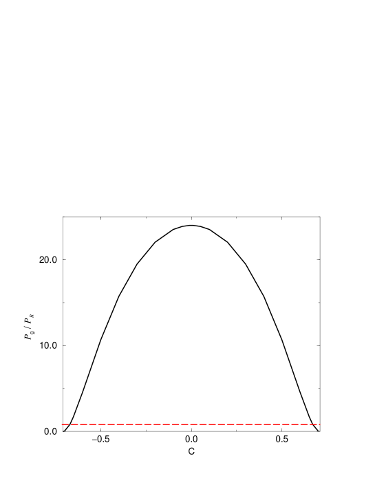
Figure 13: Tensor-scalar ratio ${\cal P}_{g}/{\cal P}_{\cal R}$ after the bounce shown against dimensionless parameter $C$ defined in Eq. (27).

The red dashed line shows the observational limit.

VI Conclusions

We have presented a simple model of a four-dimensional FRW universe that describes non-singular bouncing solutions. To do so within the context general relativity it is well-known that the null-energy condition must be violated. To achieve this we have introduced a massless “ghost” field with negative kinetic energy. A similar role is played by higher-order corrections to the low-energy string effective action which have recently been studied by Cartier Cartier who found qualitatively similar results. In order to keep the dynamics as transparent as possible we have restricted ourselves to a canonical (second-order) scalar field Lagrangian albeit with the wrong sign. Like the higher-order loop corrections, our ghost field only plays a significant dynamical role in the high energy regime close to the bounce.

We have performed a phase-plane analysis of the qualitative behaviour of expanding and contracting FRW models with both a canonical scalar field (with positive energy density) and an exponential potential plus the massless ghost field. Away from the bounce we have usual power-law expansion or contraction for a universe dominated by a scalar field with exponential potential LM85 ; Halliwell ; BB . The dimensionless slope of the potential, $\lambda$, determines the asymptotic power-law index $p=2/\lambda^{2}$ and the equation of state $w=(\lambda^{2}-3)/3$ for sufficiently flat potentials with $\lambda^{2}<6$.

It is known that for $\lambda^{2}<6$ these power-law collapse solutions describe the generic early time behaviour but are unstable at late times to kinetic-dominated collapse with $w=1$ Heard ; Gratton or to shear anisotropy Kunze . Some kind of instability is a necessary to allow an escape from the singular power-law collapse. For steep potentials with $\lambda^{2}\geq 6$ we find no non-singular solutions. But for flat potentials with $\lambda^{2}<6$ we find a class of non-singular solutions that begin in the asymptotic past as a power-law collapse, approach a minimum value of the scale factor and then approach a power-law expansion at late times.

This class of non-singular solutions provides a simple bounce model in which we then study the evolution of linear perturbations. We assume that these perturbations begin in the flat-spacetime vacuum state at early times and use this to predict the amplitude of large scale (super-Hubble) adiabatic density perturbations after the bounce.

Although both the Bardeen potential $\Phi$ and comoving curvature perturbation ${\cal R}$ evolve smoothly at the instantaneous bounce, they both have potential problems. The Bardeen potential grows rapidly during the collapse phase and is much greater than unity for the modes of interest, calling into question the validity of linear perturbation theory in the longitudinal gauge Lyth2 ; PPN1 . On the other hand the comoving gauge becomes singular whenever the total kinetic energy of the scalar fields vanishes Kodama , which occurs shortly before and after the bounce in our model.

We can however find a gauge in which the metric perturbations remain small and linear perturbation theory should be valid. In our model the massless ghost field is monotonic and provides a suitable time variable, defining a well-defined choice of gauge (the uniform $\chi$-field gauge) for perturbations. We note that we solve the regularized unconstrained evolution equations for the perturbations, using the constraint equations as a check of our numerical integration. This avoids potential problems that could arise from using the constraint equations to eliminate variables whose coefficients vanish at the bounce Cartier . We can then reconstruct the usual gauge-invariant variables from calculations in this gauge.

We find that the comoving curvature perturbation calculated during the collapse phase is a good estimator of the resulting adiabatic density perturbation on super-Hubble scales in the expanding phase. Note that the value at the end of the collapse phase is not in general the same as the that at Hubble-crossing during collapse (unlike the usual case in an inflationary expansion). This is because the dominant mode during collapse is a non-adiabatic field perturbation. However the comoving curvature perturbation remains constant on super-Hubble scales after the bounce.

By contrast the Bardeen potential calculated in the collapse phase is not a good indicator of the subsequent large scale adiabatic perturbation in the expanding phase. It is dominated by the shear in the uniform $\chi$-field gauge, which grows rapidly in the collapse phase and then decays away after the bounce, until the Bardeen potential settles down to a constant value on super-Hubble scales, related to the comoving curvature perturbation by the usual expression $\Phi=3(1+w){\cal R}/(5+3w)$. This basic point has been made by many authors Lyth ; BF ; Hwang ; LW03 and here we demonstrate it explicitly for our simple bounce model.

In particular we find that the spectral tilt of the final adiabatic curvature perturbation on super-Hubble scales in the expanding phase is given by the spectral tilt of the initial comoving curvature perturbations (or equivalently the scalar field fluctuations in the spatially flat gauge). We therefore have given an explicit model for a power-law collapse with $\lambda=\sqrt{3}$ which yields a scale-invariant of adiabatic perturbations on super-Hubble scales in the expanding phase.

The amplitude of the comoving curvature perturbation on the smallest scale (that is the minimum value of the Hubble scale during collapse) is set by the energy scale relative to the Planck scale (where vacuum fluctuations in the metric become of order unity)

$${\cal P}_{\cal R}(k=aH_{\rm max})\sim\left(\frac{H_{\rm max}}{M_{\rm Pl}}\right)^{2}\,.$$ (103)

This is very similar to the amplitude of gravitational waves (tensor perturbations) produced during collapse. The tensor-scalar ratio is an important constraint on conventional inflation models and turns out to be a severe constraint on our collapse model when $\lambda=\sqrt{3}$.

Pre big bang or collapse models have been criticised for the degree of fine-tuning required to set up the initial conditions at the start of any collapse phase Turner ; Linde ; Gratton . The dimensionless parameter $C$, defined in Eq. (27), is a first integral of the equations of motion which selects the trajectory in the homogeneous phase-space. Although any value for $|C|<1/\sqrt{2}$ yields a non-singular bounce for models with $\lambda=\sqrt{3}$, only trajectories with $|C|>0.67$ give an acceptably small tensor-scalar ratio. This provides a quantitative measure of the degree of fine-tuning of initial conditions required to get an acceptable primordial density perturbation within the class of models considered in this paper.

- (1) H. V. Peiris et al., Astrophys. J. Suppl. 148, 213 (2003) [arXiv:astro-ph/0302225].
- (2) A. R. Liddle and D. H. Lyth, 2000, Cosmological inflation and large-scale structure, Cambridge University Press.
- (3) M. Gasperini and G. Veneziano, Astropart. Phys. 1, 317 (1993) [arXiv:hep-th/9211021]; Phys. Rept. 373, 1 (2003) [arXiv:hep-th/0207130].
- (4) J. E. Lidsey, D. Wands and E. J. Copeland, Phys. Rept. 337, 343 (2000) [arXiv:hep-th/9909061].
- (5) J. Khoury, B. A. Ovrut, P. J. Steinhardt and N. Turok, Phys. Rev. D 64, 123522 (2001) [arXiv:hep-th/0103239].
- (6) R. Kallosh, L. Kofman and A. D. Linde, Phys. Rev. D 64, 123523 (2001) [arXiv:hep-th/0104073].
- (7) P. J. Steinhardt and N. Turok, arXiv:hep-th/0111030; Phys. Rev. D 65, 126003 (2002) [arXiv:hep-th/0111098].
- (8) R. Brustein, M. Gasperini, M. Giovannini, V. F. Mukhanov and G. Veneziano, Phys. Rev. D 51, 6744 (1995) [arXiv:hep-th/9501066].
- (9) D. H. Lyth, Phys. Lett. B 524, 1 (2002) [arXiv:hep-ph/0106153].
- (10) K. Enqvist and M. S. Sloth, Nucl. Phys. B 626, 395 (2002) [arXiv:hep-ph/0109214]; D. H. Lyth and D. Wands, Phys. Lett. B 524, 5 (2002) [arXiv:hep-ph/0110002]; T. Moroi and T. Takahashi, Phys. Lett. B 522, 215 (2001) [Erratum-ibid. B 539, 303 (2002)] [arXiv:hep-ph/0110096].
- (11) D. Wands, Phys. Rev. D 60, 023507 (1999) [arXiv:gr-qc/9809062].
- (12) F. Finelli and R. Brandenberger, Phys. Rev. D 65, 103522 (2002) [arXiv:hep-th/0112249].
- (13) D. H. Lyth, Phys. Rev. D 31, 1792 (1985).
- (14) N. Deruelle and V. F. Mukhanov, Phys. Rev. D 52, 5549 (1995) [arXiv:gr-qc/9503050].
- (15) J. Martin and D. J. Schwarz, Phys. Rev. D 57, 3302 (1998) [arXiv:gr-qc/9704049].
- (16) D. Wands, K. A. Malik, D. H. Lyth and A. R. Liddle, Phys. Rev. D 62, 043527 (2000) [arXiv:astro-ph/0003278].
- (17) D. H. Lyth and D. Wands, Phys. Rev. D 68, 103515 (2003) [arXiv:astro-ph/0306498].
- (18) J. Martin and P. Peter, Phys. Rev. D 68, 103517 (2003) [arXiv:hep-th/0307077]; Phys. Rev. Lett. 92, 061301 (2004) [arXiv:astro-ph/0312488]; Phys. Rev. D 69, 107301 (2004) [arXiv:hep-th/0403173].
- (19) R. Brandenberger and F. Finelli, JHEP 0111, 056 (2001) [arXiv:hep-th/0109004].
- (20) J. Khoury, B. A. Ovrut, P. J. Steinhardt and N. Turok, Phys. Rev. D 66, 046005 (2002) [arXiv:hep-th/0109050].
- (21) J. c. Hwang, Phys. Rev. D 65, 063514 (2002) [arXiv:astro-ph/0109045].
- (22) D. H. Lyth, Phys. Lett. B 526, 173 (2002) [arXiv:hep-ph/0110007].
- (23) R. Durrer and F. Vernizzi, Phys. Rev. D 66, 083503 (2002) [arXiv:hep-ph/0203275].
- (24) J. Hwang and H. Noh, Phys. Lett. B 545, 207 (2002) [arXiv:hep-th/0203193].
- (25) C. Cartier, R. Durrer and E. J. Copeland, Phys. Rev. D 67, 103517 (2003) [arXiv:hep-th/0301198].
- (26) H. Kodama and T. Hamazaki, Prog. Theor. Phys. 96, 949 (1996) [arXiv:gr-qc/9608022].
- (27) P. Peter and N. Pinto-Neto, Phys. Rev. D 66, 063509 (2002) [arXiv:hep-th/0203013].
- (28) P. Peter, N. Pinto-Neto and D. A. Gonzalez, JCAP 0312, 003 (2003) [arXiv:hep-th/0306005].
- (29) F. Finelli, JCAP 0310, 011 (2003) [arXiv:hep-th/0307068].
- (30) I. Antoniadis, J. Rizos and K. Tamvakis, Nucl. Phys. B 415, 497 (1994) [arXiv:hep-th/9305025];
- (31) C. Cartier, E. J. Copeland and R. Madden, JHEP 0001, 035 (2000) [arXiv:hep-th/9910169].
- (32) J. Martin, P. Peter, N. Pinto Neto and D. J. Schwarz, Phys. Rev. D 65, 123513 (2002) [arXiv:hep-th/0112128]; Phys. Rev. D 67, 028301 (2003) [arXiv:hep-th/0204222].
- (33) A. J. Tolley, N. Turok and P. J. Steinhardt, Phys. Rev. D 69, 106005 (2004) [arXiv:hep-th/0306109].
- (34) S. Tsujikawa, Phys. Lett. B 526, 179 (2002) [arXiv:gr-qc/0110124].
- (35) S. Tsujikawa, R. Brandenberger and F. Finelli, Phys. Rev. D 66, 083513 (2002) [arXiv:hep-th/0207228].
- (36) C. Cartier, arXiv:hep-th/0401036.
- (37) C. Cartier, J. c. Hwang and E. J. Copeland, Phys. Rev. D 64, 103504 (2001) [arXiv:astro-ph/0106197].
- (38) R. Brustein and R. Madden, Phys. Lett. B 410, 110 (1997) [arXiv:hep-th/9702043].
- (39) L. Parker, S. A. Fulling, Phys. Rev. D 7, 2357 (1973)
- (40) A. A. Starobinsky, Sov. Astron. Lett. 4, 82 (1978)
- (41) J. D. Barrow and R. A. Matzner, Phys. Rev. D 21, 336 (1980).
- (42) J. c. Hwang and H. Noh, Phys. Rev. D 65, 124010 (2002) [arXiv:astro-ph/0112079].
- (43) C. Gordon and N. Turok, Phys. Rev. D 67, 123508 (2003) [arXiv:hep-th/0206138].
- (44) N. Deruelle, arXiv:gr-qc/0404126.
- (45) N. Deruelle, A. Streich, arXiv:gr-qc/0405003.
- (46) P. Teyssandier and P. Tourrenc, J. Math. Phys. 24, 2793 (1983).
- (47) D. Wands, Class. Quant. Grav. 11, 269 (1994) [arXiv:gr-qc/9307034].
- (48) S. M. Carroll, M. Hoffman and M. Trodden, Phys. Rev. D 68, 023509 (2003) [arXiv:astro-ph/0301273]; J. M. Cline, S. y. Jeon and G. D. Moore, arXiv:hep-ph/0311312.
- (49) R. R. Caldwell, Phys. Lett. B 545, 23 (2002) [arXiv:astro-ph/9908168].
- (50) E. J. Copeland, A. R. Liddle and D. Wands, Phys. Rev. D 57, 4686 (1998) [arXiv:gr-qc/9711068].
- (51) I. P. C. Heard and D. Wands, Class. Quant. Grav. 19, 5435 (2002) [arXiv:gr-qc/0206085].
- (52) F. Lucchin and S. Matarrese, Phys. Rev. D 32, 1316 (1985).
- (53) J. J. Halliwell, Phys. Lett. B 185, 341 (1987).
- (54) A. B. Burd and J. D. Barrow, Nucl. Phys. B 308, 929 (1988).
- (55) V. F. Mukhanov, H. A. Feldman and R. H. Brandenberger, Phys. Rept. 215, 203 (1992).
- (56) K. A. Malik and D. Wands, arXiv:gr-qc/9804046.
- (57) C. Gordon, D. Wands, B. A. Bassett and R. Maartens, Phys. Rev. D 63, 023506 (2001) [arXiv:astro-ph/0009131].
- (58) J. Garcia-Bellido and D. Wands, Phys. Rev. D 53, 5437 (1996) [arXiv:astro-ph/9511029].
- (59) D. H. Lyth and E. D. Stewart, Phys. Lett. B 274, 168 (1992).
- (60) M. Sasaki, Prog. Theor. Phys. 76, 1036 (1986).
- (61) J. c. Hwang, Astrophys. J. 427, 542 (1994).
- (62) A. A. Starobinsky, JETP Lett. 30, 682 (1979) [Pisma Zh. Eksp. Teor. Fiz. 30, 719 (1979)].
- (63) S. Gratton, J. Khoury, P. J. Steinhardt and N. Turok, Phys. Rev. D 69, 103505 (2004) [arXiv:astro-ph/0301395].
- (64) K. E. Kunze and R. Durrer, Class. Quant. Grav. 17, 2597 (2000) [arXiv:gr-qc/9912081].
- (65) P. Peter and N. Pinto-Neto, Phys. Rev. D 65, 023513 (2002) [arXiv:gr-qc/0109038].
- (66) M. S. Turner and E. J. Weinberg, Phys. Rev. D 56, 4604 (1997) [arXiv:hep-th/9705035].
- (67) N. Kaloper, A. D. Linde and R. Bousso, Phys. Rev. D 59, 043508 (1999) [arXiv:hep-th/9801073].