The young stellar population in the Serpens Cloud Core:
An ISOCAM survey

We present results from an ISOCAM survey in the two broad band filters LW2 (5-8.5 $\mu$m) and LW3 (12-18 $\mu$m) of a 0.13 square degree coverage of the Serpens Main Cloud Core. A total of 392 sources were detected in the 6.7 $\mu$m band and 139 in the 14.3 $\mu$m band to a limiting sensitivity of $\sim$ 2 mJy. We identified 58 Young Stellar Objects (YSOs) with mid-IR excess from the single colour index $[14.3/6.7]$, and 8 additional YSOs from the $H-K/K-m_{6.7}$ diagram. Only 32 of these 66 sources were previously known to be YSO candidates. Only about 50% of the mid-IR excess sources show excesses in the near-IR $J-H/H-K$ diagram. In the 48 square arc minute field covering the central Cloud Core the Class I/Class II number ratio is 19/18, i.e. about 10 times larger than in other young embedded clusters such as $\rho$ Ophiuchi or Chamaeleon. The mid-IR fluxes of the Class I and flat-spectrum sources are found to be on the average larger than those of Class II sources. Stellar luminosities are estimated for the Class II sample, and its luminosity function is compatible with a coeval population of about 2 Myr which follows a three segment power-law IMF. For this age about 20% of the Class IIs are found to be young brown dwarf candidates. The YSOs are in general strongly clustered, the Class I sources more than the Class II sources, and there is an indication of sub-clustering. The sub-clustering of the protostar candidates has a spatial scale of 0.12 pc. These sub-clusters are found along the NW-SE oriented ridge and in very good agreement with the location of dense cores traced by millimeter data. The smallest clustering scale for the Class II sources is about 0.25 pc, similar to what was found for $\rho$ Ophiuchi. Our data show evidence that star formation in Serpens has proceeded in several phases, and that a “microburst” of star formation has taken place very recently, probably within the last 10⁵ yrs.

1 Introduction

The youngest stellar clusters are found deeply embedded in the molecular clouds from which they form. There are several reasons why very young clusters are particularly interesting for statistical studies such as mass functions and spatial distributions. Because mass segregation and loss of low mass members due to dynamical evolution has not had time to develop significantly for ages $\la 10^{8}$ yrs (Scalo 1998), the stellar IMF can in principle be found for the complete sample, at least for sufficiently rich clusters. For ages $\la 10^{5}$ yrs the spatial distribution should in gross reflect the distribution at birth, which gives important input to the studies of cloud fragmentation and cluster formation. Only in the youngest regions of low mass star formation do we find the co-existence of newly born stars and pre-stellar clumps, which allows one to compare the mass functions of the different evolutionary stages. Low mass stars are more luminous when they are young, being either in their protostellar phase or contracting down the Hayashi track, which permits probing lower limiting masses. Severe cloud extinction, however, requires sensitive IR mapping at high spatial resolution to sample the stellar population of embedded clusters.

ISOCAM, the camera aboard the ISO satellite (Kessler et al. 1996), provided sensitivity and relatively high spatial resolution in the mid-IR (Cesarsky et al. 1996). The two broad band filters LW2 (5-8.5 $\mu$m) and LW3 (12-18 $\mu$m), designed to avoid the silicate features at 10 and 20 $\mu$m, were selected to sample the mid-IR Spectral Energy Distribution (SED) of Young Stellar Objects (YSOs) in different evolutionary phases. According to the current empirical picture for the early evolution of low mass stars (Adams et al. 1987; Lada 1987; André et al. 1993; André & Montmerle 1994), newborn YSOs can be observationally classified into 4 main evolutionary classes. Class 0 objects are in the deeply embedded main accretion phase ($\ga$ 10⁴ yrs), and have measured circumstellar envelope masses larger than their estimated central stellar masses, with overall SEDs resembling cold blackbodies and peaking in the far-IR. Class I sources ($\sim 10^{5}$ yrs) are observationally characterised by a broad SED with a rising spectral index towards longer wavelengths ($\alpha_{\rm IR}>0$) in the mid-IR. The Class II sources spend some 10⁶ yrs in a phase where most of the circumstellar matter is distributed in an optically thick disk, displaying broad SEDs with $-1.6<\alpha_{\rm IR}<0$. At $\alpha_{\rm IR}\approx-1.6$ the disk turns optically thin, and the sources evolve into the ($\sim 10^{7}$ yrs) Class III stage where the mid-IR imprints of a disk eventually disappear. A normal stellar photosphere has $\alpha_{\rm IR}=-3$. Thus, while Class 0 objects are not favourably traced by mid-IR photometry, they are expected to be rare. At the other extreme, Class III sources cannot generally be distinguished using mid-IR photometry since most of them have SEDs similar to normal stellar photospheres. But mid-IR photometry from two broad bands, as obtained in this study with ISOCAM, is highly efficient when it comes to detection and classification of Class I and Class II sources. Thus, considering the fact that these latter objects constitute the major fraction of the youngest YSOs, the ISOCAM surveys provide a better defined sample for statistical studies than e.g. near-IR surveys for regions with very recent star formation (see Prusti 1999).

This paper presents the results from an ISOCAM survey of $\sim$ 0.13 square degrees around the Serpens Cloud Core in two broad bands centred at 6.7 and 14.3 $\mu$m. This cloud, located at $b^{\rm II}=5^{\circ}$ and $l^{\rm II}=32^{\circ}$ at a distance of $259\pm 37$ pc (Straiz̆ys et al. 1996; Festin 1998), comprises a deeply embedded, very young cluster with large and spatially inhomogeneous cloud extinction, exceeding 50 magnitudes of visual extinction. Only a few sources are detected in the optical (Hartigan & Lada 1985; Gómez de Castro et al. 1988; Giovannetti et al. 1998). Serpens contains one of the richest known collection of Class 0 objects (Casali et al. 1993; Hurt & Barsony 1996; Wolf-Chase et al. 1998; Davis et al. 1999), an indication that this cluster is young and active. On-going star formation is also evident from the presence of several molecular outflows (Bally & Lada 1983; White et al. 1995; Huard et al. 1997; Herbst et al. 1997; Davis et al. 1999), pre-stellar condensations seen as sub-mm sources (Casali et al. 1993; McMullin et al. 1994; Testi & Sargent 1998; Williams & Myers 2000), a far-IR source (FIRS1) possibly associated with a non-thermal triple radio continuum source (Rodriguez et al. 1989; Eiroa & Casali 1989; Curiel et al. 1993), a FUor-like object (Hodapp et al. 1996), and jets and knots in the 2.1 $\mu$m H₂ line (Eiroa et al. 1997; Herbst et al. 1997). Investigations of the stellar content have been made with near-IR surveys (Strom et al. 1976; Churchwell & Koornneef 1986; Eiroa & Casali 1992; Sogawa et al. 1997; Giovannetti et al. 1998; Kaas 1999a), identifying YSOs using different criteria, such as e.g. near-IR excesses, association with nebulosities, and variability.

In this paper we identify new cluster members, characterize the YSOs into Class I, flat-spectrum, and Class II sources, estimate a stellar luminosity function for the Class II sample and search for a compatible IMF and age, and finally describe the spatial distribution of both the protostars and the pre-main sequence population in this cluster.

Table 1: Observational parameters, detection statistics and photometric results for each of the 6 ISOCAM rasters CE, CW, CS, D1, D2, D3. See Fig. 10 and text.

$$\alpha$$(2000) (2000) Size¹ T_int pfov n N_det N_6.7 N_14.3 N_both 1 1

(′ ′) (sec) (″) (mJy) (mJy)

(1) (2) (3) (4) (5) (6) (7) (8) (9) (10) (11) (12) (13)

CE 18 29 48.3 01 16 04.5 1313 0.28 3/6 413 133 113 56 51 2 3

CW 18 29 06.3 01 16 01.4 1313 2.1 6 7 152 139 43 38 0.8 2

CS 18 29 52.5 01 02 37.9 1316.5 0.28 6 413 165 152 41 34 1.2 4

D1 18 29 48.7 01 15 20.5 1.84.6 2.1 3 44 20 15 9 9 1 2

D2 18 29 52.3 01 15 20.8 1.84.6 2.1 3 44 24 19 11 10 1 4.5

D3 18 29 57.8 01 12 55.4 4.61.8 2.1 3 44 30 21 15 13 1 3

Tot² 421 392 140 124

¹ Approximate size since each raster has tagged edges.
² The total number is corrected for multiply observed sources in overlapped regions.

2 Observations and reductions

2.1 ISOCAM

This work presents data from the two ISOCAM star formation surveys LNORDH.SURVEY_1 and GOLOFSSO.D_SURMC. These were surveys within the ISO central programme mapping selected parts of the major nearby star formation regions in the two broad band filters LW2 (5-8.5 $\mu$m) and LW3 (12-18 $\mu$m). Other results on young stellar populations based on these surveys comprise the Chamaeleon I, II and III regions (Nordh et al. 1996; Olofsson et al. 1998; Persi et al. 2000), the $\rho$ Ophiuchi star formation region (Bontemps et al. 2001), the R Corona Australis region (Olofsson et al. 1999), and the L1551 Taurus region (Gålfalk et al. 2004), all observations performed basically in the same way. Data reduction methods were generally the same for all regions, using a combination of the CIA (CAM Interactive Analysis) package and own dedicated software. For overviews of survey results, see Nordh et al. (1998), Kaas & Bontemps (2000), and Olofsson (2000).

In the Serpens Core region about 0.13 square degrees (deg$2$) were covered at 6.7 and 14.3 $\mu$m in 3 separate, but overlapping main rasters named CE, CW and CS (see Fig. 10). In addition, 3 smaller fields within CE (named D1, D2, and D3) were observed at a higher sensitivity. CE covers the well known Serpens Cloud Core, CW is a reference region to the west of the Core which is substantially opaque in the optical but without appreciable 60 $\mu$m IRAS emission (Zhang et al. 1988a), and CS is a region directly to the south of the Cloud Core which has a peak in the 60 $\mu$m flux. The rasters were always made along the right ascension, with about half a frame (90″) overlap in $\alpha$ and 24$\arcsec$ overlap in $\delta$. For the larger rasters the pixel field of view (PFOV) was set to the nominal survey value of 6$\arcsec$ except for the CE region in LW2, where a PFOV of 3$\arcsec$ was selected because of the risk of otherwise saturating the detector. Also in order to avoid saturation, the intrinsic integration time was set to $T_{\rm int}=0.28$ s except for field CW where the nominal survey value of $T_{\rm int}=2.1$ s was used. Each position in the sky was observed during about 15 s. For the deeper imaging within CE the overlap was 72$\arcsec$ in $\alpha$ and $\delta$, and each position was observed during about 92 s. The individual integration time was $T_{\rm int}=2.1$ s and a PFOV of 3$\arcsec$ was used for better spatial resolution. See Table 1 for an overview.

2.1.1 Image reduction

Each raster consists of a cube of frames which is reduced individually, and in total 9112 individual frames were analysed. The dark current was subtracted using the CAL-G dark from the ISOCAM calibration library and, if necessary, further improved by a second order dark correction using a FFT thresholding method (Starck et al. 1996a). Cosmic ray hits were detected and masked by the multiresolution median transform (MMT) method (Starck et al. 1996b). The transients in the time history of each pixel due to the slow response of the LW detector were treated with the IAS inversion method v.1.0 (Abergel et al. 1996a, b). Flat field images were constructed from the observations themselves. See Starck et al. (1999) for a general description of ISOCAM data processing.

2.1.2 Point source detection and photometry

Bright point sources, even well below the saturation level, produce strong memory effects which are not entirely taken out by the transient correction. Due to the large PFOV which undersamples the point spread function (PSF), also remnants of cosmic ray glitches may be mistaken for faint sources. By looking at the time history of the candidate source fluxes, however, it is easy to distinguish real sources from memory effects, glitches or noise. This is done for each individual sky coverage, the redundancy being 2-6. Both the source detection and the photometry was made with the interactive software developed by our team. See also previous papers on this survey (Nordh et al. 1996; Olofsson et al. 1999; Persi et al. 2000; Bontemps et al. 2001).

The fluxes of each verified source were measured by aperture photometry, with nominal aperture radii 1.5 and 3 pixels, for the 6$\arcsec$ and 3$\arcsec$ PFOV, respectively, and aperture correction applied using the empirical PSF. For each redundant observation (2-6 overlaps) the flux is the median flux from the $N_{\rm ro}$ readouts per sky position. The sky level was estimated from the median image to reduce the noise. Uncertainties are estimated both from the standard deviation around this median (i.e. the temporal noise and also a measure of the efficiency of the transient correction method) and from the $\sigma$ of the sky background (i.e. the spatial noise). The quoted flux uncertainties are these two contributions added in quadrature. The photometric scatter between the overlaps is estimated and deviating measurements are discarded. If a source is affected by the dead column (no 24 was disconnected) or is hit by a serious glitch or memory effect in one of the redundant overlaps, this one is skipped, and the remaining ones are used to estimate the flux. If the redundancy is not sufficient (i.e. along raster edges), then the fluxes are flagged if affected by the dead column, detector edges, glitches, memory effects, close neighbours etc.

Source positions were calculated from that of the redundant images where the source is closest to the centre, in order to diminish the effects of field distortion. The source centre is taken to be the peak pixel, and the default ISO pointing was used as a first source position value. The ISO position was then compared to near-IR positions of known sources in the literature (Eiroa & Casali 1992; Sogawa et al. 1997; Giovannetti et al. 1998), and ISO positions of bright optical sources to the digital sky survey. Bulk offsets found for each raster registration were then corrected. The maximum bulk offset found was 5$\arcsec$, and we estimated an average uncertainty of $\pm 3\arcsec$ in RA and DEC. When 2MASS became available we checked the positions of 61 sources in Table 2 which have 2MASS counterparts and are not multiples unresolved by ISOCAM. The median deviation between ISOCAM and 2MASS positions is $2.2\arcsec$. One star deviates by as much as $9.2\arcsec$ (ISO-356), and 5 more sources by more than $4.5\arcsec$ (these are ISO-29, 207, 272, 357 and 367).

2.1.3 Photometric Calibration

The two broad band filters LW2 and LW3 have defined reference wavelengths at 6.7 and 14.3 $\mu$m, respectively. The fluxes in ADU/s are converted to mJy through the relations 2.32 and 1.96 ADU/gain/s/mJy for the bands LW2 and LW3, respectively (from in-orbit latest calibration by Blommaert et al. (2000)). These flux conversions are strictly valid only for sources with F${}_{\nu}\propto\nu^{-1}$, however, and therefore a small colour correction must be applied to the blue sources (cf. Sect. 3.2 for blue vs. red). This correction is obtained by dividing the above conversion factors by 1.05 and 1.02 for LW2 and LW3, respectively, yielding the effective factors 2.21 and 1.92 ADU/gain/s/mJy for blue sources.

Conversion from flux density to magnitude is defined as m${}_{\rm 6.7}=-2.5\log(F_{\nu}(6.7\mu m)/82.8)$ and m${}_{\rm 14.3\mu m}=-2.5\log(F_{\nu}(14.3)/18.9)$, where $F_{\nu}$ is given in Jy. The $\sim 5$ % responsivity decrease throughout orbit has not been corrected for.

2.2 Nordic Optical Telescope near-IR imaging

A $6\arcmin\times 8\arcmin$ region inside Serp-CE, the area which is usually referred to as the Serpens Cloud Core and has been covered to a smaller or larger extent by several studies in the near-IR (Eiroa & Casali 1992; Sogawa et al. 1997; Giovannetti et al. 1998; Kaas 1999a), was mapped deeply in $J$ (1.25 $\mu$m), $H$ (1.65 $\mu$m) and $K$ (2.2 $\mu$m) in August 1996, only 4 months after the ISOCAM observations. See Fig. 10 for the location of the different maps. Also, a region to the NW of the $JHK$ field has been mapped in the $K$ band, see Fig. 4, but with a total coadded integration time from only 30 sec to 1 min. These observations were made with the ARcetri Near Infrared CAmera (Arnica) at the 2.56m Nordic Optical Telescope, La Palma. See Kaas (1999a) for details on this near-IR dataset.

2.3 IRAM 30m Telescope Observations

A 1.3 mm dust continuum mosaic of the Serpens main cloud core was taken with the IRAM 30-m telescope equipped with the MPIfR 37-channel bolometer array MAMBO-I (Kreysa et al. 1998) during four night observing sessions in March 1998. The passband of the MAMBO bolometer array has an equivalent width $\approx 70$ GHz and is centered at $\nu_{eff}\approx 240$ GHz.

The $\sim 19^{\prime}\times 6^{\prime}$ mosaic consists of eleven individual on-the-fly maps which were obtained in the dual-beam raster mode with a scanning velocity of 8$\arcsec$/sec and a spatial sampling of 4$\arcsec$ in elevation. In this mode, the telescope is scanning continuously in azimuth along each mapped row while the secondary mirror is wobbling in azimuth at frequency of 2 Hz. A wobbler throw of 45$\arcsec$ or 60$\arcsec$ was used. The typical azimuthal size of individual maps was 4$\arcmin$. The size of the main beam was measured to be $\sim$ 11$\arcsec$ (HPBW) on Uranus and other strong point-like sources such as quasars. The pointing of the telescope was checked every $\sim 1$ hr using the VLA position of the strong, compact Class 0 source FIRS1 (good to $\sim 0.1\arcsec$ – Curiel et al. (1993)); it was found to be accurate to better than $\sim$ 3$\arcsec$. The zenith atmospheric optical depth, monitored by ‘skydips’ every $\sim 2$ hr, was between $\sim 0.2$ and $\sim 0.4$. Calibration was achieved through on-the-fly mapping and on-off observations of the primary calibrator Uranus (e.g. Griffin & Orton 1993, and references therein). In addition, the Serpens secondary calibrator FIRS1, which has a 1.3 mm peak flux density $\sim 2.4$ Jy in an 11$\arcsec$ beam was observed before and after each map. The relative calibration was found to be good to within $\sim 10\%$ by comparing the individual coverages of each field, while the overall absolute calibration uncertainty is estimated to be $\sim 20\%$.

The dual-beam maps were reduced and combined with the IRAM software for bolometer-array data (“NIC”; cf. Broguière, Neri & Sievers (1995)) which uses the EKH restoration algorithm (Emerson, Klein & Haslam 1979).

3 ISOCAM results

3.1 Source statistics, sensitivity and completeness

Table 1 gives an overview of the observational parameters and the results of the point source photometry for each of the six rasters named in col. 1. Columns 2, 3 and 4 give the centre position and size of the raster fields. Columns 5, 6 and 7 give the unit integration times, the PFOV and the average number of readouts per sky position. Column 8 gives the total number of source detections. Columns 9 and 10 give the number of sources for which photometry was obtained at 6.7 and 14.3 $\mu$m, respectively. Column 11 gives the number of sources with flux determinations in both of the photometric bands. Columns 12 and 13 give the measured 1$\sigma$ photometric limits which are about 4 and 6 times the read-out-noise for the large and the deep fields, respectively. Practically all sources detected at 14.3 $\mu$m are also detected at 6.7 $\mu$m, but there are 15 cases of 14.3 $\mu$m detections without 6.7 $\mu$m counterparts. On the average, only 30% of the 6.7 $\mu$m detections are also detected at 14.3 $\mu$m, but this value is clearly larger for the CE field. The sensitivity, which depends on the PFOV and T_int as well as the amount of nebulosity and bright point sources, is lowered by memory effects from bright sources in the CE field and by the presence of a nebula in the CS field. For the deep fields (D1, D2, D3) the main limiting factor in terms of sensitivity is the memory effect and the fact that the flat fields are based on fewer frames.

The deep fields within the CE area are independently repeated observations (observed within the same satellite orbit), and therefore permit a check of the photometric repeatability for a number of sources. The median values of the individual direct scatter between the measured fluxes were found to be: about 30% for the 6.7 $\mu$m band measured from 28 sources between 4 mJy and 2 Jy, and about 15% for the 14.3 $\mu$m band, measured from 14 sources between 30 mJy and 5.7 Jy (note different pixel scale). This corresponds to a median error of 0.13 dex in the $[14.3/6.7]$ colour index, which is in good agreement with the scatter (of sources without mid-IR excesses) around the value expected for normal photospheres (see Fig. 2) at a flux density of 10 mJy in the 14.3 $\mu$m band.

To estimate how many field stars to expect at a given sensitivity within the observed fields, the stellar content in a cone along the line-of-sight was integrated in steps of 0.02 kpc out to a distance of 20 kpc. The Galaxy was represented by an exponential disk, a bulge, a halo and a molecular ring, following Wainscoat et al. (1992). Absolute magnitudes at 2.2 $\mu$m (M_K) and in the 12 $\mu$m IRAS band (M₁₂), local number densities and scale heights of the different stellar populations, as well as their contribution to the different components of the Galaxy were provided by Wainscoat et al. (1992) in their model of the mid-IR point source sky. Absolute magnitudes at 7 $\mu$m, M₇, are estimated by linear interpolation between M_K and M₁₂.

Figure 1: Histograms of sources at 6.7 $\mu$m (left) and 14.3 $\mu$m (right) for the CW field (upper) and the total sample (lower). The boldface steps in the lower panels correspond to the population of mid-IR excess sources. The expected number of galactic sources in each bin, normalised to each field, from modelling the stellar content in a cone along the line-of-sight is inserted for zero cloud extinction (solid lines), A${}_{V}\approx 5$ (dotted lines), and A${}_{V}\approx 10$ (dashed lines).

The upper panels of Fig. 1 show the histograms of the 6.7 $\mu$m and 14.3 $\mu$m sources in the CW field, which is free of nebulosity and practically free of IR excess sources. The bin size of 0.2 in $\log F_{\nu}$ corresponds to 0.5 magnitudes. Inserted are the model counts of galactic sources at 7 and 12 $\mu$m, scaled to the CW field size. The expected source number per bin is calculated assuming no cloud extinction (solid line), an average extinction of 0.2 magnitudes in the 6.7 $\mu$m band (dotted line), and A_6.7 = 0.4 magnitudes (dashed line), corresponding to roughly A${}_{V}\sim 5$ and A${}_{V}\sim 10$, respectively (cf. Sects. 4 and 5 about extinction). For the CW field an average cloud extinction of A${}_{V}\sim 7-8$ magnitudes is in agreement with the location of the majority of the sources in a DENIS $I-J/J-K^{\prime}$ diagram, as well as an extinction map based on R star counts (Cambrésy 1999). Comparing the number of observed sources at 14.3 $\mu$m with the model expectation at 12 $\mu$m indicates completeness at $\sim$ 6 mJy or m_14.3 = 8.7 mag. The observations at 6.7 $\mu$m are estimated to be complete to $\sim$ 5 mJy or m_6.7 = 10.6 mag. The lower panels of Fig. 1 show the histograms for the total sample. The boldface steps show the contribution of the mid-IR excess sources. The dashed line represents the model expectation assuming an average cloud extinction of about 10 magnitudes of visual extinction, i.e. A_6.7 = 0.41 mag and A_14.3 = 0.36 mag (cf. Sects. 4 and 5). Thus, the whole sample taken together, and allowing for a subtraction of the mid-IR excess sources, indicates an overall completeness at $\sim$ 6 mJy for the 6.7 $\mu$m band and at 8 mJy for the 14.3 $\mu$m band (i.e. at m_6.7 = 10.4 mag and m_14.3 = 8.5 mag).

Figure 2: The colour index $[14.3/6.7]$ defined as $\log(F_{\nu}^{14.3}/F_{\nu}^{6.7})$ is shown on the y-axis and the flux $F_{\nu}^{14.3}$ also given in magnitudes $m_{14}$ is shown on the x-axis. The SED index between 6.7 and 14.3 $\mu$m is given on the right hand y-axis. 53 sources with substantial IR excess are located above $[14.3/6.7]=-0.2$ or $\alpha_{\rm IR}^{7-14}=-1.6$ (dotted line). While 28 of these were previously suggested as YSOs, 25 are new YSO candidates (filled circles).

3.2 Sources with mid-IR excesses

For the 124 sources with fluxes in both bands we present a colour magnitude diagram in Fig. 2. The colour index $[14.3/6.7]$, defined as $\log(F_{\nu}^{14.3}/F_{\nu}^{6.7})$, is plotted against $F_{\nu}^{14.3}$. This colour index can be converted to the commonly used index of the Spectral Energy Distribution (SED):

$$\alpha_{\rm IR}^{7-14}=\frac{\log(\lambda_{14}F_{\lambda_{14}})-\log(\lambda_{7}F_{\lambda_{7}})}{\log\lambda_{14}-\log\lambda_{7}},$$ (1)

calculated between 6.7 and 14.3 $\mu$m and indicated on the right hand y-axis. The completeness limit is given with solid lines as the combined effect of the completeness in each of the two bands.

The sources tend to separate into two distinct groups, with some few intermediate objects. The “red” sources (circles) are interpreted as pre-main-sequence (PMS) stars surrounded by circumstellar dust. This sample is not believed to be contaminated with galaxies. At the completeness flux level of 8 mJy at 14.3 $\mu$m the expected extracalagtic contamination is about half a source within our map coverage and at the level of 3 mJy (the faintest source in our sample at 14.3 $\mu$m) the contamination is below two sources within the mapped region (Hony 2003). No correction for extinction has been made on these numbers, so that they should be considered as upper limits to the extragalactic contamination.

We have decided to set the division line between mid-IR excess objects and “blue” objects (triangles) at $[14.3/6.7]=-0.2$ or $\alpha_{\rm IR}^{7-14}=-1.6$ (dotted line), which corresponds to the classical border between Class II and Class III objects (cf Sect 5).

Table 2: The 77 ISOCAM sources identified as YSOs in the Serpens cluster.

ISO $$\alpha_{2000}$$ Other ID

# 18^h mag mag mag mJy mJy mJy mJy

29 28^m525 1^∘1247 1^g 0.6 3 2

150 29^m306 1^∘0109 19 3 21 5

158 29^m317 1^∘0822 10 1 16^m 7 BD+01 3687

159 29^m320 1^∘1842 8.41 0.01 1162 28 2351 26 IRAS 18269+0116

160 29^m320 1^∘1834 9.82 0.01 114 2 - - IRAS 18269+0116

173 29^m334 1^∘0828 64 2 110 20 [CDF88] 6

202 29^m399 1^∘1755 11.80 0.01 8 2 12^c 3

207 29^m411 1^∘0740 56 1 68 3 STGM3

216 29^m423 1^∘2019 12.02 0.01 6 3 14^c 2

219 29^m437 1^∘0722 7 2 - - STGM2

221 29^m443 1^∘0455 2652 37 3664 23 IRAS 18271+0102

224 29^m448 1^∘1310 13.22 0.01 12.26 0.01 11.82 0.01 7 2 - - EC11

226 29^m448 1^∘1544 - - 15.45 0.02 13.51 0.01 3 1 - - EC13

231 29^m460 1^∘1623 18.12 0.09 13.86 0.01 11.81 0.01 11 4 - - EC21

232 29^m463 1^∘1214 13.22 0.01 11.66 0.01 10.99 0.01 6 4 - - EC23

234 29^m469 1^∘1610 - - 18.73 0.14 14.47 0.02 7 3 - - EC26

237 29^m472 1^∘1626 - - 16.51 0.03 13.19 0.01 33 3 27 5 EC28

241 29^m481 1^∘1643 - - - - 16.11 0.05 28 4 41 8

242 29^m486 1^∘1342 18.14 0.10 14.94 0.01 13.14 0.01 5 2 4 1 K8,EC33

249 29^m491 1^∘1632 - - 17.09 0.05 13.62 0.01 143^f 6 637^f 9 EC37

250 29^m493 1^∘1619 - - - - 11.67 0.01 2242^f 54 4464^f 35 DEOS

252 29^m499 0^∘5612 21 1 31 3

253 29^m496 1^∘1457 - - - - 14.90 0.03 49 13 49 5 EC40

254 29^m495 1^∘1707 12.46 0.01 156 12 214 5 EC38

258a 29^m496 1^∘1528 - - 17.77 0.08 14.80 0.03 19^f 2 24^f 4 EC41,GCNM23

258b 29^m503 1^∘1521 - - - - - - - - 13^f 4

259 29^m506 1^∘0135 29 13 - -

260 29^m505 1^∘1417 - - - - 16.76 0.15 3 1 - -

265 29^m512 1^∘1642 15.35 0.04 12.90 0.01 11.32 0.01 766 13 813 16 EC53

266 29^m513 1^∘1317 15.90 0.02 14.27 0.01 13.02 0.01 2 1 - - GCNM35,EC51

269 29^m522 1^∘1321 - - 14.79 0.01 13.31 0.01 2 1 - - K16,EC56

270 29^m522 1^∘1549 - - - - 17.70 0.20 9 2 44 8

272 29^m525 1^∘1254 19.01 0.22 14.63 0.01 12.54 0.01 3 1 - - EC59

276 29^m529 1^∘1456 - - - - 14.80 0.03 74 12 231 4 GCNM53

277 29^m532 1^∘1543 - - - - 14.88 0.03 9 2 - - EC63

279 29^m534 1^∘1313 - - 14.15 0.01 13.60 0.01 1 2 - - STGM14,EC66

283 29^m536 1^∘1700 - - 11.58^a 0.01 10.63^a 0.01 30 4 29 6 EC67

285 29^m539 1^∘1332 16.58 0.04 14.21 0.01 12.87 0.01 6^d 1 6 3 GCNM63,EC68

287 29^m541 1^∘0714 3 1 4 3

289 29^m544 1^∘1503 16.15 0.06 12.66 0.01 10.86 0.01 19 9 - - EC69,CK10

291 29^m544 1^∘1444 14.26 0.01 13.32 0.01 12.74 0.01 2 2 - - GCNM70,EC70

294 29^m551 1^∘1322 16.32 0.03 13.84 0.01 12.39 0.01 19 3 31 12 EC73,GEL3

298 29^m556 1^∘1431 14.78 0.02 12.21 0.01 10.44 0.01 100 27 119^d 16 EC74,CK9,GEL4

304 29^m566 1^∘1301 14.86 0.01 12.55 0.01 11.38 0.01 33 5 38 3 EC79,GEL5

306 29^m566 1^∘1240 - - 17.90 0.08 13.75 0.02 43 4 32 4 EC80

307 29^m568 1^∘1446 12.01 0.01 10.20 0.01 8.63 0.01 680^e,d 10 1762^e,d 43 SVS2,CK3,EC82

308 29^m568 1^∘1318 - - - - 16.62 0.19 11.0 2 - - K32,HCE170/171

309 29^m568 1^∘1249 15.15 0.02 12.44 0.01 11.00 0.01 45 4 70 3 EC84,GEL7

312 29^m575 1^∘1259 15.56^b 0.03 13.61^b 0.01 11.24^b 0.01 453 8 697 10 EC88+EC89

313 29^m575 1^∘1349 17.81 0.12 15.47 0.04 13.46 0.03 32 3 - - GCNM94,EC87

314 29^m575 1^∘1407 12.10 0.01 9.16 0.01 7.03 0.01 4479 97 6388 50 SVS20,CK1,EC90

317 29^m578 1^∘1252 15.30^b 0.02 11.47^b 0.01 9.45^b 0.01 332 5 1039^d 35 EC92+EC95

318 29^m578 1^∘1237 - - 14.22 0.01 11.47 0.01 100^f 9 105^f 20 EC94

319 29^m577 1^∘1531 15.95 0.03 12.67 0.01 10.59 0.01 45 4 - - EC93,CK13

320 29^m578 1^∘1229 - - 15.61 0.02 12.91 0.01 23 7 19 5 EC91

321 29^m582 1^∘1522 12.97 0.01 10.92 0.01 9.48 0.01 204 9 327^d 5 CK4,GEL12,EC97

322 29^m583 1^∘1249 - - 14.61 0.01 12.25 0.01 32 3 - - EC98

326 29^m587 1^∘1426 16.62 0.06 13.82 0.01 11.56 0.01 202 39 335^f 8 EC103

(continued on next page)

ISO $$\alpha_{2000}$$ Other ID

# 18^h mag mag mag mJy mJy mJy mJy

327 29^m589 1^∘1231 - - - - 15.41 0.04 9.7 2.0 8.1 4.3 HCE175

328 29^m592 1^∘1406 11.78 0.01 10.36 0.01 9.46 0.01 223 23 186^f 10 EC105,CK8,GEL13

330 29^m595 1^∘1159 - - - - 14.37 0.02 423 7 643 9 HB1

331 29^m597 1^∘1313 - - - - 15.37 0.04 145 9 346 12

338 30^m007 1^∘1338 13.40 0.01 11.15 0.01 10.07 0.01 16 4 - - EC117,CK6,GEL15

341 30^m011 1^∘1326 - - 15.39 0.02 12.90 0.01 20 3 24 11 EC121

345 30^m021 1^∘1400 17.16 0.06 14.74 0.01 12.88 0.01 24 4 50 7 EC125,CK7

347 30^m028 1^∘1228 15.11 0.02 11.72 0.01 9.69 0.01 499^c 12 658 13 EC129

348 30^m032 1^∘1617 12.14 0.01 10.89 0.01 10.15 0.01 41ⁿ 11 59^d 3 EC135,GGD29

351 30^m040 1^∘1238 16.51 0.03 13.54 0.01 12.13 0.01 8.4 1.9 - - EC141

356 30^m052 1^∘1244 16.08 0.03 14.51 0.01 13.53 0.01 2.5 1.6 - - K40,EC152

357 30^m058 1^∘0622 10 1.7 18 2.3

359 30^m064 1^∘0109 32 4 47 4

366 30^m076 1^∘1204 12.20 0.01 10.74 0.01 9.92 0.01 53 7 64 5 STGM8

367 30^m081 1^∘0142 12ⁿ 5 19ⁿ 4

370 30^m084 0^∘5848 61 3 83 4 double in I

379 30^m093 1^∘0247 99 5 67 6

393 30^m112 1^∘1240 12.97^b 0.01 11.67^b 0.01 11.06^b 0.01 6.3 4.1 11.2 4.5

407 30^m139 1^∘0855 2.2 1.3 4.9 5.3

^a $H$ and $K$ band data from the Arnica 1995 map, which is slightly displaced from the 1996 map and therefore includes this object.
^b ISOCAM source is resolved into two sources in the near-IR, and the near-IR fluxes are added.
^c Flux measurement affected by proximity to the dead column. If the dead column cannot be avoided by any of the redundant observations, this flagging. If source is located on the dead column, a flux measurement is not attempted at all.
^d Source close to the detector edge in all redundant observations.
^e Extended source.
^f ISOCAM source is not quite resolved from a bright neighbour.
^g Galaxy contamination? For fluxes $\sim$ 3 mJy at 14.3 $\mu$m the “red” sample is expected to contain less than two galaxies in our field according to Hony (2003).
^m Flux might be affected by memory effects from other sources.
ⁿ Nebulous sky background.

Empty space means no measurement available in this work, while a hyphen means no detection.

Identifier acronyms are related to the following references: SVS (Strom et al. 1976); GGD (Gyulbudaghian et al. 1978); HL (Hartigan & Lada 1985); CK (Churchwell & Koornneef 1986); GEL (Gómez de Castro et al. 1988); CDF (Chavarria-K et al. 1988); EC (Eiroa & Casali 1992); SMM (Casali et al. 1993); MMW (McMullin et al. 1994); HHR (Hodapp et al. 1996); HB (Hurt & Barsony 1996); STGM (Sogawa et al. 1997); HCE (Horrobin et al. 1997); GCNM (Giovannetti et al. 1998); K (Kaas 1999)

Table 3: The 71 “blue” ISOCAM sources which have $[14.3/6.7]<-0.2$. Many of these are likely to be field stars, but some could be young cluster members of Class III type. Colour correction applied.

ISO $$\alpha_{2000}$$ Other ID

# 18^h mag mag mag mJy mJy mJy mJy

2 28^m41.2 1^∘1515 30 5 12 2

4 28^m41.9 1^∘1406 35 5 6.4 2.9

7 28^m42.1 1^∘1431 26 3 7.9 3.0

9 28^m43.6 1^∘1610 19 3 8.0 2.2

11 28^m45.1 1^∘1019 10 2 3.3 3.1

12 28^m45.2 1^∘1650 57 8 11 2

16 28^m47.0 1^∘1036 53 6 13 2

20 28^m48.4 1^∘1314 37 6 9 2

24 28^m49.7 1^∘1909 60 7 15 2

31 28^m52.6 1^∘1010 5^d 1 1.2 2.8

42 28^m58.3 1^∘1055 20 2 3.5 1.7 [SCB96] 41

46 28^m59.8 1^∘0958 27 4 4.8 2.5

49 29^m 0.3 1^∘1817 114 14 32^f 4

61 29^m 3.4 1^∘1834 28 4 8 2

63 29^m 3.8 1^∘1039 26 4 4.7 2.5

65 29^m 4.6 1^∘2002 33 3 8 2

66 29^m 4.7 1^∘1615 56 6 15 2

69 29^m 5.0 1^∘2204 28 3 7 2

74 29^m 8.1 1^∘1235 13 2 2.4 1.2

80 29^m 9.6 1^∘0929 12 18 4.1^d 2.0

82 29^m10.6 1^∘1830 27 3 6.3 1.8

84 29^m10.6 1^∘1806 12 2 3.8 2.5

91 29^m12.4 1^∘1120 23 3 5.3 1.9

94 29^m13.4 1^∘1159 118 12 33 4

96 29^m14.2 1^∘2130 31 4 8.3 2.3

98 29^m14.9 1^∘2155 79 13 19 4

102 29^m15.8 1^∘ 932 128 22 34 5

104 29^m16.9 1^∘1837 28 2 7.0 2.0

112 29^m19.9 1^∘2059 65 8 38 5

126 29^m25.6 1^∘0350 59 2 12 4

132 29^m26.8 1^∘1156 21 2 5.0 2.7

134 29^m27.3 1^∘1258 15 2 1.4 2.5 BD+01 3686

140 29^m28.6 1^∘1024 51 2 15 2

144 29^m29.4 1^∘1403 49 7 12 2

145 29^m29.7 1^∘1309 37 6 9.0 2.5

153 29^m30.9 1^∘1518 10 2 0.9 2.1

166 29^m32.6 1^∘0946 20 2 7.0 2.6

184 29^m37.2 1^∘0915 125 3 37 6

189 29^m37.7 1^∘1118 67 2 31 2

190 29^m37.6 1^∘1130 68 10 32 3

191 29^m37.9 1^∘0036 44^c 2 10 3

208 29^m41.0 1^∘1240 36 6 9 4 SVS18

209 29^m41.1 1^∘2056 8.69 0.01 44 5 12 2

210 29^m41.5 1^∘1000 12 2 6 4

228 29^m45.2 1^∘1846 10.09 8.67 0.01 91 9 19 3 SVS 9

238 29^m47.6 1^∘0512 1414 19 285 7 StRS 208

243 29^m48.9 1^∘1143 11.18 0.01 9.53 0.01 8.84 0.01 35 4 8 3 SVS3

244 29^m49.2 0^∘5854 20 3 7^e 3

255 29^m49.9 1^∘0924 91 2 24 4

264 29^m51.6 0^∘5621 14 2 5 1

267 29^m51.6 1^∘1032 48 3 13 6 SVS 5

271 29^m52.7 1^∘0438 24 6 4 6

290 29^m54.3 1^∘1747 27 5 4 2

296 29^m55.8 1^∘0414 118 5 31 4

300 29^m56.1 1^∘0024 53 19 12 13

311 29^m57.6 1^∘1046 26 2 15 3 BD+01 3689B

(continued on next page)

ISO $$\alpha_{2000}$$ Other ID

# 18^h mag mag mag mJy mJy mJy mJy

324 29^m58.4 1^∘2026 15 3 4 3 SVS 16

332 30^m 0.2 1^∘0947 62 2 36 4

334 30^m 0.0 1^∘2155 160 10 40 3 SVS 15

337 30^m 0.6 1^∘1519 19.13 0.279 12.61 0.004 8.92 0.001 340 8 95 6 CK2,EC118

339 30^m 0.8 1^∘1941 70 7 15 2 SVS 13

342 30^m 1.6 0^∘5930 40 9 8 6

349 30^m 3.7 1^∘ 452 97 6 21 9

372 30^m 8.4 0^∘5529 80 2 19 4

375 30^m 8.7 0^∘5516 98 3 28 5

378 30^m 9.0 1^∘1444 11.81 0.003 9.68 0.001 8.67 0.001 70 7 14 4 SVS7

382 30^m 9.2 1^∘1753 7 2 3 4

389 30^m10.4 1^∘1936 18 2 5 4 BD+01 3693

401 30^m12.1 1^∘1641 11.39 0.003 9.59 0.001 8.64 0.001 66 11 13 5 SVS6

409 30^m14.7 1^∘0524 15 3 5 3

410 30^m14.7 1^∘0617 22 2 7 3

^b Binary or close companion not quite resolved by ISOCAM.
^c Flux measurement affected by proximity to the dead column. If the dead column cannot be avoided by any of the redundant observations, this flagging. If source is located on the dead column, a flux measurement is not attempted at all.
^d Source close to the detector edge in all redundant observations.
^e Extended source.

Identifier acronyms are related to the following references: SVS (Strom et al. 1976); CK (Churchwell & Koornneef 1986); StRS (Stephenson 1992); EC (Eiroa & Casali 1992), SCB (Straizys et al. 1996).

Except for a few transition objects, the “blue” group (triangles) is mainly located at the colour index of normal photospheres, i.e. $[14.3/6.7]=-0.66$ or $\alpha_{\rm IR}^{7-14}=-3$ (dashed line). The spread around this value indicates the increasing photometric uncertainty with decreasing flux, although some of the scatter might be real. M giants have intrinsic excesses in the colour index $[14.3/6.7]$ of less than 0.1, while late M giants are expected to have excesses of up to $\sim 0.2$ above normal photospheres. Although late M giants are few, a number of M giants are expected in the observed sample of field stars. Thus, the slight displacement of this group of sources above the colour of normal photospheres could be due to a combination of extinction and intrinsic colours of M giants. The effect of extinction is small, however. A reddening vector of size corresponding to A${}_{K}=3$ is indicated in the figure. (More about extinction in Sect. 4.)

This same dichotomy in colour was found also in the Chamaeleon dark clouds (Nordh et al. 1996), in RCrA (Olofsson et al. 1999), and in $\rho$ Ophiuchi (Bontemps et al. 2001). According to the SED index, $\alpha_{\rm IR}^{7-14}$, the mid-IR excess sources are Class II and Class I types of Young Stellar Objects (YSOs). In Chamaeleon I about 40% of the mid-IR excess sources had been previously classified as Classical T Tauri stars (CTTS), and in $\rho$ Ophiuchi $\sim$ 50% were previously known as Class II and Class Is. In Serpens, very few sources are optically visible and the IRAS data suffer badly from source confusion. The known YSOs are thus a sample of sources classified from near-IR excesses, association with nebulosity, emission-line stars, ice features, clustering properties, and variability (Eiroa & Casali 1992; Hodapp et al. 1996; Horrobin et al. 1997; Sogawa et al. 1997; Giovannetti et al. 1998; Kaas 1999a). Previously known YSOs are not found in the “blue” group, although Class III sources, young stars with marginal or no IR excess, have their locus there. A few objects in the transition phase between Class II and Class III are evident in the “blue” group. Class III sources without IR excess cannot be distinguished from field stars purely on the basis of broad band infrared photometry. They can, however, be efficiently identified through X-ray observations.

The fact that intrinsic IR excess is so easily distinguished from reddening at these wavelengths, enables an unambiguous classification of the youngest YSOs on the basis of one single colour index $[14.3/6.7]$. In this way ISOCAM found $53$ Class I and Class II YSOs, of which only $28$ had been previously suggested as YSO candidates.

Positions and photometry of the 53 Class I and Class II YSOs are listed among other members of the Serpens Core cluster in Table 2. The 71 “blue” sources are listed in Table 3. Many of these are field stars, but some are likely to be young cluster members of Class III type. Fig. 1 shows that the CW region contains as many as 20 (10) sources detected at 6.7 $\mu$m (14.3 $\mu$m) above the expected field star contribution according to the galactic model by Wainscoat et al. (1992). Because there are only two IR excess sources in the CW field, of which one is very faint, these are practically all belonging to the “blue” sample. Since the total region surveyed is about 3 times as large as the CW field, perhaps more than 20 “blue” sources from Table 3 could be Class IIIs belonging to the cluster.

4 Near-IR and mid-IR excess YSOs

When it comes to detecting IR excesses, the $J$ band usually limits the number of sources in a $J-H/H-K$ diagram because of its sensitivity to extinction. For the ISOCAM observations the 14.3 $\mu$m band is the less sensitive, unless the sources are extremely red (see limits in Fig. 2). Using the $H-K/K-m_{6.7}$ diagram as in Olofsson et al. (1999), however, we should be able to detect more IR excess objects. Fig. 3 shows that practically all sources with excesses in the colour index $[14.3/6.7]$ are also found to have excesses in their $K-m_{6.7}$ index. Approximate intrinsic colours of main-sequence, giant and supergiant stars, taken from the source table of Wainscoat et al. (1992) and interpolated between 2.2 and 12 $\mu$m, are given as boldface curves (solid, dotted and dashed, respectively).

Sources with ISOCAM mid-IR excesses (circles) separate well from those without mid-IR excesses (triangles). A reddening vector has been calculated by fitting a line from origin through the 4 sources without mid-IR excesses. The slope (1.23) is mainly constrained by the star CK2, which is believed to be a background supergiant, see e.g. Casali & Eiroa (1996). On the basis of a number of background stars in the $J-H/H-K$ diagram, Kaas (1999a) found a reddening law of the form A${}_{\lambda}\sim\lambda^{-1.9}$ to fit the Serpens data. Extrapolation of this law to 6.7 $\mu$m would give a slope of 0.83 in the $H-K/K-m_{\rm 6.7}$ diagram, which is in disagreement with all the 4 sources without mid-IR excess. The A${}_{\lambda}\sim\lambda^{-1.7}$ law (Whittet 1988) gives an even shallower slope. By assuming, however, the A${}_{\lambda}\sim\lambda^{-1.9}$ law to hold for $H$ and $K$, and using the empirical slope found in Fig. 3, the extinction in the 6.7 $\mu$m band is estimated to be A${}_{\rm 6.7}=0.41$ A_K. This is in good agreement with the values 0.37, 0.35 and 0.47 found by Jiang et al. (2003) from the ISOGAL survey, whose three values depend on the actual form of the near-IR extinction curve applied.

Figure 3: The $H-K/K-m_{\rm 6.7}$ diagram of the Serpens Cloud Core with individual error bars for each source, and some $H$ upper limits (arrows). The IR excess sources from Fig. 2 are encircled. The intrinsic colours of main-sequence (bold solid), giants (bold dotted), and supergiant (bold dashed) stars cluster close to (0,0). A reddening vector (solid line) is estimated on the basis of the four sources without $[14.3/6.7]$ excess (triangles). Eight additional IR excess YSOs (numbered) were found in this diagram, i.e. displaced by more than 1$\sigma$ to the right of the reddening band (dotted vector).

As shown in Kaas & Bontemps (2000) only about 50% of the IR excess sources which display clear excesses in the single ISOCAM colour index $[14.3/6.7]$ show up as IR excess objects in the $J-H/H-K$ diagram. This was demonstrated by plotting the same sources in the two diagrams, using a statistically significant sample of several hundred sources in Serpens, $\rho$ Ophiuchi, Chamaeleon I, and RCrA. This result implies that a sole use of the $J-H/H-K$ diagram will severely underestimate the IR-excess population of YSOs in active star formation regions. Bontemps et al. (2001) showed that in $\rho$ Ophiuchi only 50% of the 123 Class II sources have near-IR excesses large enough to be recognizable in the $J-H/H-K$ diagram. Similarly we confirm here specifically for Serpens that the mid-IR excess sources cluster along the reddening line when plotted in a $J-H/H-K$ diagram, and that only 50% would be recognized as having IR excesses from JHK data alone.

The $H-K/K-m_{7}$ diagram is more efficient than the $J-H/H-K$ diagram in distinguishing between intrinsic circumstellar excess (circles) and reddening (triangles). Thus, by sampling the SED a bit more into the mid-IR, the use of two colour indices to select sources with intrinsic IR excesses becomes substantially less prone to the influence from cloud extinction. Fig. 3 also shows that the mid-IR excesses apparent from the $[14.3/6.7]$ index, always appear already at 6.7 $\mu$m, but only in half of the cases at 2.2 $\mu$m.

In addition to the $53$ IR excess sources obtained from Fig 2, another eight sources were found to have IR excess from the $H-K/K-m_{7}$ diagram, i.e. displaced by more than 1$\sigma$ to the right of the reddening band (dotted line). This means we find 25% more IR excess sources within the centre region than by using the $[14.3/6.7]$ index alone.

Class II sources are most likely Classical T Tauri stars (CTTS), but we can not exclude that some of them are weak-lined T Tauri stars (WTTS). Among the Class II sources detected with ISOCAM in Chamaeleon I about 1/3 had been previously classified as WTTS (Nordh et al. 1996). For WTTS one could attribute the presence of mid-IR excess but a lack of near-IR excess to an inner hole in the circumstellar disk (Moneti et al. 1999). CTTS, on the other hand, are believed to have inner disks, since they show strong H$\alpha$ emission, which is commonly interpreted as a signature of the accretion process onto the surface of the object, but could also arise in stellar winds. Optical information is scarce in the Serpens Cloud Core because of the large cloud extinction, and we do not know what fraction of the Class IIs are strong H$\alpha$ emitters. It is well known from studies of CTTS locations in the $J-H/H-K$ diagram (Lada & Adams 1992; Meyer et al. 1997), that many CTTS lack detectable near-IR excesses; about 40% in Taurus-Auriga according to Strom et al. (1993).

For typical CTTS the near-IR wavelength region is strongly dominated by the photospheric emission, and rather large amounts of dust hot enough to produce a strong excess at 2 $\mu$m are therefore needed in order to distinguish intrinsic IR excess from the effects of scattering and extinction in the $J-H/H-K$ diagram. In a region such as the Serpens Cloud Core, where 7 of the Class IIs in question here were originally proposed to be YSOs due to their association with nebulosity (Eiroa & Casali 1992), it is likely that scattered light in the J and H bands adds to the lack of detectable near-IR excesses as it gives a bluer $H-K$ colour index.

From an ISOCAM sample of CTTS with mid-IR excesses in Chamaeleon I, Comerón et al. (2000) found evidence for the presence of near-IR excesses to be correlated with luminosity, suggesting an incapability of objects with very low temperatures and luminosities (young brown dwarfs and very low mass CTTS) to raise the temperature needed at the inner part of the circumstellar disk to produce a detectable excess at 2.2 $\mu$m, in agreement with model predictions (Meyer et al. 1997). The majority of the Serpens sources are substantially more luminous. As pointed out by Hillenbrand et al. (1998), the larger the stellar radius (i.e. the younger the star is), the more difficult it is to separate near-IR excesses from the stellar flux. This could perhaps be part of the explanation for the youngest sources (e.g. two flat-spectrum sources without near-IR excess). But we found all the Class I sources to possess near-IR excesses, such that the role of larger radii in these cases seems to be well compensated for, probably by their larger disk accretion rates. A statistical interpretation based on broad band photometry is likely over-simplified, however, and there are many properties intrinsic to the star-disk system (such as disk inclination angle, disk accretion rate, stellar mass and radius) which contribute to the complexity of the individual YSOs. From the results presented here for Serpens, in Bontemps et al. (2001) for $\rho$ Ophiuchi, and in Kaas & Bontemps (2000) for the ISOCAM star formation surveys in general, it is evident that one should be careful in estimating disk frequencies among YSOs based on near-IR excesses only, see also Haisch et al. (2001). Since our study samples only IR excess objects, we cannot say anything about the disk fraction among YSOs in Serpens.

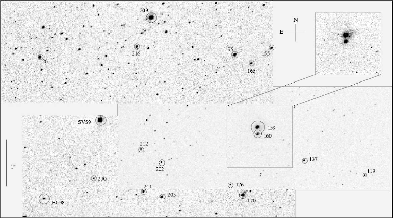
Figure 4: Arnica $K$ band mapping of the region to the NW of the $JHK$ field. ISOCAM sources are encircled and their identifications given. Sources 159, 202, 216 and EC38 are YSOs with $[14.3/6.7]$ colour excess. Sources SVS9 and 209 are without such an excess. The remaining sources are not detected at 14.3 $\mu$m. See Sect. A.

5 Characterization of the YSO population

5.1 Large fraction of Class I sources

We have combined the photometry from ISOCAM with the available $K$ band photometry from 1996 (Kaas 1999a) and calculated the two SED indices: $\alpha_{\rm IR}^{2-14}$ and $\alpha_{\rm IR}^{2-7}$, which are plotted against each other in Fig. 5 for the 39 mid-IR excess sources and the 6 sources without mid-IR excesses. The index $\alpha_{\rm IR}^{2-14}$ is close to the index originally used to define the three classes I, II and III from the shape of their SED between 2.2 and 10 (or 25) $\mu$m by Lada & Wilking (1984); Lada (1987). Figure 5 indicates the loci of these classes in addition to a transitional class referred to as ”flat spectrum” sources.

According to the updated IR spectral classification scheme (André & Montmerle 1994; Greene et al. 1994) we tentatively define YSOs with $\alpha_{\rm IR}^{2-14}>0.3$ as Class I sources, those with $-0.3<\alpha_{\rm IR}^{2-14}<0.3$ as flat-spectrum sources, and objects with $-1.6<\alpha_{\rm IR}^{2-14}<-0.3$ as Class II sources. There is a marginal hint of a gap in the distribution of sources along the $[14.3/6.7]=-0.2$ axis at $\alpha_{\rm IR}^{2-14}\approx 0.3$, which was seen also in the $\rho$ Ophiuchi sample (Bontemps et al. 2001), though at $\approx 0.5$. It is apparent that we cannot distinguish between Class III sources and field stars. (The transition sources in the “blue” group (see Fig. 2) with some mid-IR excesses are all located outside the field for which we have K-band observations.)

IR excess sources without detection at 14.3 $\mu$m (see Sec. 4.2) can be classified from the approximately linear relation between $\alpha_{\rm IR}^{2-14}$ and $\alpha_{\rm IR}^{2-7}$ found in Fig. 5. In this case Class Is are those which have $\alpha_{\rm IR}^{2-7}>1.2$, corresponding to $K-m_{7}>4.8$, Class IIs are those which have $\alpha_{\rm IR}^{2-7}<-0.25$, corresponding to $K-m_{7}<3.2$, and flat-spectrum sources are those in between. Thus, the total number of sources in each category is larger than apparent from Fig. 5. From Fig. 3 we have 1 more Class I, 2 more flat-spectrum sources, and 5 more Class IIs. Three sources (260, 277 and 308) have only $K$ and 6.7 $\mu$m detections, but their very red colours strongly suggest membership in the Class I category.

Figure 5: The spectral index $\alpha_{\rm IR}^{2-7}$ versus $\alpha_{\rm IR}^{2-14}$, or equivalently, the $K-m_{7}/K-m_{14}$ colour diagram, for a subset of the ISOCAM sample. The locations of Class I, Class II and Class III sources and field stars are indicated. Note the relatively large fraction of Class I sources in this diagram.

The number of Class I sources ($19$) is thus about equal to the number of Class II sources ($18$) in the central part of the Serpens cluster. This is very unusual since Class II sources outnumber Class I sources by typically 10 to 1 in star formation regions. If we include the $13$ ”flat spectrum” sources in the Class II group, the Class I/Class II number ratio is still as high as $19/31$. This is exceptional, also compared to the results obtained from ISOCAM surveys in other regions; in Chamaeleon I this number ratio is $5/{\bf 42}$ (Kaas 1999b) and in $\rho$ Ophiuchi: $16/123$ (Bontemps et al. 2001). Such a large population of Class I sources indicates a recent burst of star formation in this region and would be in line with the rich collection of Class 0 objects found in this cluster by Casali et al. (1993) and Hurt & Barsony (1996).

5.2 Reddening effect on the $\alpha_{\rm IR}^{2-14}$ index?

While a spectral index between two fixed wavelengths, such as 2.2 and 14.3 $\mu$m, is practical and provides a preliminary classification for a large number of sources, a truly reddening-independent classification is obtainable only when complete SEDs are available over the $\sim$ 2 to 100 $\mu$m range (or to 1.3 mm if Class 0 sources are involved). In the following we discuss the possibility that sources defined as Class Is from the $\alpha_{\rm IR}^{2-14}$ index could be heavily extinguished Class II or flat-spectrum sources.

The source CK2 (probably a background supergiant) is seen through more than 50 magnitudes of visual extinction (Kaas 1999a), and indicates an empirical slope (=1.6) of the extinction law in Fig. 5, as do five other sources without mid-IR excesses. This reddening line translates to a slope of $0.92$ in the $K-m_{7}/K-m_{14}$ diagram, which gives the relation A₁₄ = 0.88 A₇ in terms of magnitudes, by using the relation $A_{7}=0.41A_{K}$ obtained in Sect. 4. It is remarkable that the group of mid-IR excess sources are lined up along the same slope as the one outlined by the reddened field stars. In this sense, some of the sources classified as Class I objects on the basis of Fig. 5 could be interpreted as highly extinguished Class II objects, either deeply embedded in the cloud or seen edge-on. Flat-spectrum sources and Class IIs are generally expected to be optically visible objects. In Serpens, however, only one (ISO-Ser-159) of the 13 flat-spectrum sources and only three of the 18 Class IIs are optically visible. This shows the extreme degree of embeddedness, and is in agreement with the C¹⁸O map of White et al. (1995), which suggests that the visual cloud extinction is larger than 30 magnitudes everywhere in the NW-SE ridge and may reach values as high as $A_{V}\sim 200$ in some places. The fact that the slopes are so similar suggests that Class Is are either merely more embedded Class IIs, or that the extinction behaves roughly in the same way for Class I envelopes as for the cloud in general at these wavelengths. This would be in line with Padgett et al. (1999) who observed three Class I SED YSOs with HST/NICMOS and found edge-on disks in all three cases.

As shown in Fig. 2 the $\alpha_{\rm IR}^{7-14}$ index is rather insensitive to extinction. As many as 15 YSOs in our sample have $\alpha_{\rm IR}^{2-14}>0$, but $\alpha_{\rm IR}^{7-14}<0$, among them the well known DEOS. For some of these we have more spectral information than the three flux points at 2.2, 6.7 and 14.3 $\mu$m. The two sources HB1 and EC129 are relatively isolated YSOs both in the near-IR and mid-IR images and should not suffer so much from the source confusion that sets a limit to the usefulness of IRAS data for the other sources. We use HIRES IRAS fluxes and upper limits from Hurt & Barsony (1996) and extend our mid-IR SEDs to longer wavelengths. Figure 6 shows that both HB1 and EC129 (HB2) have rising spectra beyond a clear dip in the SED at $\sim$ 14 $\mu$m. These sources have clearly Class I SEDs, but the dip at $\sim$ 14 $\mu$m will produce a blue $\alpha_{\rm IR}^{7-14}$ index.

Figure 6: SEDs of HB1 and EC129. The flux points at 25, 60 and 100 $\mu$m are taken from Hurt & Barsony (1996). Note that the 60 and 100 $\mu$m points for EC129 are upper limits only.

Hurt & Barsony (1996) divided the flux from their HIRES map of IRAS 18272+0114 between the three sources DEOS, EC53 and S68N, while ISOCAM resolves six mid-IR excess sources (cf Fig. 11), of which only EC37 has $\alpha_{\rm IR}^{7-14}>0$.

It is possible that a broad silicate absorption feature and/or the presence of H₂O and CO₂ ices in the 14.3 $\mu$m band (Whittet et al. 1996; de Graauw et al. 1996) may cause absorption effects that correspond in magnitude to the observed dips in the SEDs at $\sim$ 14 $\mu$m, noting that the effect is there for the most deeply embedded sources. Recently, ISOCAM-CVF spectroscopy of 42 Class I and Class II YSOs in Serpens, $\rho$ Ophiuchi, Chamaeleon and RCrA by Alexander et al. (2003) reveals a number of absorption features from 5 to 18 $\mu$m. They find that the majority of Class I sources fall in their category a, having deep absorption features of ices and silicates, and conclude that in the cases of large extinction the continuum spectral index between 2 and 14 $\mu$m provides a truer value of the shape of the underlying continuum than the observed mid-IR spectrum. For the sub-sample of 20 sources that were studied by Alexander et al. (2003) in Serpens we found: four Class Is, six flat-spectrum sources, four Class II sources, one “blue” source, and we did not detect five of their sources. All four Class Is, three flat-spectrum sources, and one Class II fall in their group a, and two flat-spectrum sources and three Class IIs in their category b (only SVS2 is of type c). This comparison shows overall good agreement, and indicates that we have not overestimated the number of Class Is in our study.

Also, the presence of shocked molecular H₂ line emission in the 6.7 $\mu$m band (e.g. Cabrit et al. 1998; Larsson et al. 2002) included in the measured flux of some of the youngest sources could contribute to give a bluer $\alpha_{\rm IR}^{7-14}$ index than expected from a dust continuum.

Recent 2-D models of Class I source geometries by Whitney et al. (2003) which include flared disk and bipolar cavity produce mid-IR SEDs with very broad dips around 10 $\mu$m, and overall much bluer mid-IR colours than produced by simple 1D or simplified 2-D models.

Figure 7: The average flux at 6.7 and 14.3 $\mu$m versus $\alpha_{\rm IR}^{2-14}$ for a subset of the ISOCAM sample. The location of Class I, Class II and Class III sources and field stars are indicated. Filled circles mark the 15 YSOs with $\alpha_{\rm IR}^{2-14}>0$ and $\alpha_{\rm IR}^{7-14}<0$.

Based on the previous discussion we trust that the $\alpha_{\rm IR}^{2-14}$ index gives a more reliable measure of the SED than the $\alpha_{\rm IR}^{7-14}$ index. We have also looked at the mid-IR fluxes of Class Is versus Class IIs. If all the 15 YSOs with $\alpha_{\rm IR}^{2-14}>0$ and $\alpha_{\rm IR}^{7-14}<0$ were reddened Class II sources, one would expect them to be on the average fainter than (or at most as bright as) the YSOs with $\alpha_{\rm IR}^{2-14}<0$. We note, however, that there is a slight tendency that sources with large $\alpha_{\rm IR}^{2-14}$ indices also are, on the average, the brightest ones in the mid-infrared. Figure 7 shows the average flux at 6.7 and 14.3 $\mu$m versus $\alpha_{\rm IR}^{2-14}$, with a reddening vector of A${}_{K}=3$ magnitudes inserted. The filled circles in the figure mark the 15 sources that have $\alpha_{\rm IR}^{2-14}>0$ and $\alpha_{\rm IR}^{7-14}<0$. Excluding the flat-spectrum sources, the median fluxes are $0.18$ and $0.029$ Jy for 15 Class Is and 27 Class IIs (including all those from Table 6 that have mid-IR fluxes), respectively. For comparison, the median mid-IR fluxes of 16 Class Is and 76 Class IIs in $\rho$ Ophiuchi are $1.17$ and $0.095$ Jy, respectively (Bontemps et al. 2001). In Chamaeleon I for 5 Class Is and 42 Class IIs these numbers are $0.28$ and $0.077$ Jy, respectively. While the statistics is low for the Chamaeleon I Class I sources, there is an indication of luminosity evolution from the Class I to the Class II phase, the case being strongest for $\rho$ Ophiuchi. We conclude that on the basis of this statistical luminosity argument, there seems to be an intrinsic difference between the Class I and the Class II populations.

Noting that Class Is are on the average more luminous in the mid-IR than Class IIs (cf. Bontemps et al. 2001), we caution that it is not entirely excluded that the large number fraction of Class I sources in Serpens could be a direct effect of a lower sensitivity because of a larger distance. There are about 80 faint YSO candidates in the Serpens Cloud Core below the sensitivity limit of ISOCAM (Kaas 1999a).

Although the exact Class I/Class II number ratio might become subject to modification when future observations at high spatial resolution and sensitivity towards longer wavelengths are available (SIRTF-Spitzer at 24 $\mu$m and FIRST-Herschel at 90-250 $\mu$m), we believe that the main conclusion of an unusually large fraction of Class I sources in the Serpens Cloud Core will be maintained.

5.3 The protostar sample in Serpens

Based on the discussion in the previous paragraph, we have arrived at a sample of 20 Class I SED sources which are listed in Table 4 with the two SED indices $\alpha_{\rm IR}^{2-14}$ and $\alpha_{\rm IR}^{2-7}$. These are all protostar candidates. Although Class 0 sources normally are not expected to be detectable at shorter wavelengths than about 25 $\mu$m, we detect two Class I sources, ISO-241 and ISO-308, within the $\pm$ 3$\arcsec$ positional uncertainties of S68N and SMM4, respectively.

Motte & André (2001) found that about 60% of the Class I sources in Taurus-Auriga are “true protostars”, using the criterion that the envelope mass to stellar mass fraction is $\ga 0.1$. A similar method has been applied to the Serpens data. But first we exclude 3 sources in order to account for the possible confusion with Class 0 sources (in the case of EC41) or contribution of Class 0 sources (in the cases: ISO-241, ISO-308) in the sample of 19 Class Is in the region mapped by IRAM. The fraction of bona-fide protostars in the Serpens Core is then estimated to be 9 out of 16 Class Is or 56%, with an uncertainty of $\pm$ 10% because of source confusion problems with the strong clustering.

Table 4: The 20 Class I sources. $\Delta K$ and fwhm refers to measured variability 1995-1996 (Kaas 1999a) and extendedness in the K-band, respectively. K-band magnitudes from 1996 are found in Table 2.

ISO	Other ID	$\alpha_{IR}^{2-14}$	$\alpha_{IR}^{2-7}$	fwhm	$\Delta K$
#				$\arcsec$	mag
270		2.56	3.54	2.31
331		2.51	4.12	4.57
330	HB1	2.35	4.26	1.47	0.32
250	DEOS	2.06	3.52	7.52	0.92
276	GCNM53	2.02	3.05	1.89
249	EC37	1.98	2.66	1.25	0.26
241		1.74	3.26	1.49
308	HCE170/1711	-	2.84	4.48	0.64
253	EC40	1.23	2.76	1.21
265	EC53	0.98	2.27	2.27	0.59
259		-	1.942	-
260		-	1.88	1.83
258a	EC41	0.96	1.81	1.33
312	EC88/893	0.85	1.73	9.53	0.11
254	EC38	0.82	1.78	1.004	-
326	EC103	0.62	1.27	1.55	0.22
327	HCE175	0.53	1.73	1.42
306	EC80	0.44	1.70	1.32
277	EC63	-	1.21	1.26
313	GCNM94	-	1.19	1.32	0.43

¹ both are extended, HCE171=K32 is variable
² Ks = 14.48 from 2MASS PSC, 16” south-west of extended IRAS 18273+0059, possible K extendedness not investigated
³ both are extended, EC88 is variable
⁴ from image serp-nw which has better seeing

Identifier acronyms as in Table 2.

Extended, elongated and polarized near-IR emission is predicted by models of infalling envelopes which have developed cavities owing to bipolar outflows, where near-IR radiation from the central object may escape and scatter off dust in the cavity and the outer envelope, see e.g. Whitney et al. (1997). Park & Kenyon (2002) find that 70% of the bona-fide protostars in Taurus are extended in the near-IR, and that less than 10% of the sources that are extended in the near-IR show no extension in mm continuum. Our near-IR data has a spatial resolution about 10 times better than the IRAM map, and we have included in Table 4 the full width at half maximum (fwhm) of a gaussian fit to the source profiles in the $K$ band images. The median fwhm of 160 isolated and relatively bright sources over the field is $1.\arcsec 27\pm 0.\arcsec 10$. Sources with a fwhm greater than $1.\arcsec 6$, i.e. above 3$\sigma$, are here defined as extended in the K-band. For the Class I sources this concerns 8 of 19 sources or 42%, highly coinciding with continuum sources except for ISO-331 and ISO-260. There are no extended sources in the flat-spectrum and Class II samples.

Substantial K-band variability was found in 8 of the above Class I sources, 5 of the flat-spectrum sources and 5 of the Class II sources (Kaas 1999a). The brightness variations of the Class I sources are given in Table 4 as $\Delta K$. The median value of the amplitude is $0.38\pm 0.27$ mag, larger than the variations found for Class Is in Taurus (Park & Kenyon 2002).

Table 5: The 13 flat-spectrum sources. $\Delta K$ and fwhm refers to measured variability 1995-1996 (Kaas 1999a) and extendedness in the K-band, respectively. K-band magnitudes from 1996 are found in Table 1.

ISO	Other ID	$\alpha_{IR}^{2-14}$	$\alpha_{IR}^{2-7}$	fwhm	$\Delta K$
#				$\arcsec$	mag
234	EC26	-	0.63	1.31
322	EC98	-	0.17	1.31
345	EC125	0.26	0.44	1.30
317	EC92/95	0.19	-0.03	1.35
159	IRAS 18269+0116	0.11	0.23	1.001	-
237	EC28	0.07	0.99	1.23
307	SVS2	0.06	-0.06	1.38	0.19
347	EC129	0.06	0.53	1.34
314	SVS20 (double)	-0.03	0.30	2.742	0.14
318	EC94	-0.05	0.56	1.35
341	EC121	-0.14	0.30	1.27	0.21
294	EC73	-0.24	-0.18	1.31	0.66
320	EC91	-0.24	0.45	1.33	0.32

¹ From image serp-nw which has better seeing.
² Double source, not extended.

Identifier acronyms as in Table 2.

The flat-spectrum sources are believed to be in a transition phase between the Class I and the Class II stage, but a few of these might be found to be true protostars. We have listed them in Table 5 with SED indices, $K$-band fwhm and variability amplitude. Both SVS2 and SVS20 have centrosymmetric polarization patterns, indicating that evacuated bipolar cavities surround them, and both are double sources (Huard et al. 1997). Among the flat-spectrum sources ISO-159, EC129, SVS20, and ISO-237 (i.e. 30%) are detected as mm continuum sources in our IRAM map.

Table 6: The 43 ISOCAM YSOs found to be Class II sources or candidates. A hyphen for the SED indices means no detection at 14 $\mu$m. $A_{K}$ is the derived extinction in the K-band, and $L_{\star}$ is the stellar luminosity estimated as explained in Sect. 6. $\Delta K$ is the amplitude of the K-band variability 1995-1996 (Kaas 1999a). None of the sources for which Arnica $K$ images were available was found to be extended in $K$.

ISO	Other ID	$\alpha_{IR}^{2-14}$	$\alpha_{IR}^{2-7}$	$A_{K}$	$L_{\star}$	Additional information
#				(mag)	($L_{\odot}$)
29		-2.13	-3.96	0.32	0.009	Mid-IR excess, $Ks=11.17$ from 2MASS
150		-1.30	-1.59	0.30	0.19	15” north of radio source S68 3, $Ks=10.69$ from 2MASS
158	BD+01 3687	-1.88	-2.92	0.0	0.086	$K=9.8$ from Chavarria-K et al. (1988). Transition object II-III?
160		-	-0.69	2.28	2.4	See Appendix A
173	[CDF88] 6	-1.58	-2.46	0.0	0.57	$Ks=9.21$ from 2MASS
202		-1.05	-1.42	0.77	0.096	Located 30” south-east of HH460
207	STGM 3	-1.18	-1.48	0.35	0.57	$Ks=9.64$ from 2MASS, NIR excess (Sogawa et al. 1997)
216		-0.86	-1.47	0.0	0.057	Located 1’ east of HH477
219	STGM 2	-	-1.70	0.58	0.077	$Ks=11.60$ from 2MASS, NIR excess (Sogawa et al. 1997)
221	IRAS 18271+0102	-1.14	-1.53	1.09	36	$Ks=5.38$ from 2MASS, see also Clark (1991)
224	EC11	-	-1.58	0.11	0.062	Clear IR excess in the $H-K/K-m_{7}$ diagram
226	EC13	-	-0.84	$\sim$ 2.0	0.061	Clear IR excess in the $H-K/K-m_{7}$ diagram
231	EC21	-	-1.18	3.30	0.33	Uncertain, see Appendix A
232	EC23	-	-2.33	0.69	0.072	Uncertain, See Appendix A
242	K8,EC33	-1.02	-0.80	2.28	0.099	Variable, $\Delta K=0.21$
252		-0.87	-1.15	0.70	0.24	$Ks=11.12$ from 2MASS
266	GCNM35,EC51	-	-1.77	0.76	0.021	NIR excess
269	K16,EC56	-	-1.58	$\sim$ 1.7	0.029	Variable, $\Delta K=0.21$
272	EC59	-	-1.82	3.42	0.086	Uncertain, see App.A
279	STGM14,EC66	-	-1.56	$\sim$ 1.4	0.020	Variable, $\Delta K=0.21$ + NIR excess
283	EC67	-1.14	-1.22	$\sim$ 0.51	0.32
285	GCNM63,EC68	-0.89	-0.77	1.47	0.097
287		-0.80	-1.04	0.75	0.030	Mid-IR excess + optically visible, likely Class II
289	EC69,CK10	-	-1.42	2.56	0.45	See Appendix A
291	GCNM70,EC70	-	-2.05	0.09	0.016	NIR excess
298	EC74,CK9,GEL4	-0.48	-0.29	1.67	1.7	Variable, $\Delta K=0.15$
304	EC79,GEL5	-0.64	-0.52	1.42	0.50
309	EC84,GEL7	-0.49	-0.55	1.80	0.79
319	EC93,CK13	-	-0.89	2.35	0.97	Clear IR excess in the $H-K/K-m_{7}$ diagram
321	CK4,GEL12,EC97	-0.42	-0.44	1.16	2.8
328	EC105,CK8,GEL13	-0.73	-0.38	0.55	2.4	Variable, $\Delta K=0.63$
338	EC117,CK6,GEL15	-	-2.21	1.36	0.25	No IR excess, but ass. with nebulosity
348	EC135,GGD29	-1.01	-1.34	0.39	0.42
351	EC141	-	-1.12	2.05	0.16	Clear IR excess in the $H-K/K-m_{7}$ diagram
356	K40,EC152	-	-1.03	0.70	0.030	Clear IR excess in the $H-K/K-m_{7}$ diagram
357		-1.11	-1.73	0.25	0.096	$Ks=11.23$ from 2MASS
359		-0.92	-1.20	0.38	0.33	$Ks=10.56$ from 2MASS, strong H$\alpha$ emission (to be publ.)
366	STGM8	-1.08	-1.29	0.59	0.59
367		-0.87	-1.16	0.34	0.12	$Ks=11.67$ from 2MASS, strong H$\alpha$ em.
370		-0.83	-1.00	0.02	0.54	$Ks=10.13$ from 2MASS, dbl in the optical, both H$\alpha$ em. (to be publ.)
379		-1.95	-2.24	0.81	1.2	$Ks=8.09$ from 2MASS
393		-1.44	-2.27	0.44	0.066	double in $K$
407		-1.24	-2.13	0.19	0.021	$Ks=12.36$ from 2MASS

Identifier acronyms as in Tab 2.

5.4 The pre-main sequence sample in Serpens

Based on the ISOCAM YSO sample found in Table 1 we have used a combination of criteria to arrive at a tentative sample of Class II sources in Serpens. These are listed in Table 6 with SED indices, whenever available, and additional criteria used to argue for a Class II status. Since our $K$ imaging from 1996 only covers about 10% of the ISOCAM survey, we have also used published $K$ band photometry whenever available to calculate the SED indices. Also, we have assumed that if the source shows strong mid-IR excess and is optically visible, it is more likely to be a Class II than a flat-spectrum or Class I type of YSO. As a supporting argument for Class II designation we have found for a few mid-IR excess sources without JHK data, strong H$\alpha$ in emission (to be published in a future paper). When the 2MASS All-Sky Data Release became available while we were finalizing our investigation, we used the near-IR photometry from their point source catalogue for the Class II source candidates where such data was lacking, and found spectral indices in agreement with our above reasoning.

The pre-main sequence population also includes the Class III type of YSOs, objects which show no IR signatures of an optically thick disk. Since the basic criterion for selecting YSOs in our study is IR excess, we do not sample these sources. With the existing photometric data alone we cannot distinguish Class IIIs from field stars, except for a few objects in the transition zone between the Class II and Class III phases. The clear gap between the two groups formed in the ISOCAM colour-magnitude diagram in Fig. 2 demonstrates that there are few objects undergoing this transition, i.e. that the transition must be rapid. This is evident in all the star formation regions surveyed by ISOCAM. In Serpens at least five sources from Table 3 belong to this transition group, cf. Fig. 2, and we list them as candidate Class IIIs in Table 7. None of these are located in the central Cloud Core region covered by Arnica deep near-IR imaging.

Table 7: Five candidate Class III sources from Table 3. These are probably in the transition phase between Class II and III having some remaining IR excess. K-band magnitudes for two sources are obtained from Kaas et al. (1995).

ISO	Other ID	$\alpha_{IR}^{7-14}$	$\alpha_{IR}^{2-14}$	$\alpha_{IR}^{2-7}$
#
112		-1.67
190		-1.98	-1.83	-1.73
210		-2.00
311	BD+01 3689B	-1.73	-2.21	-2.54
332		-1.72

Identifier acronyms as in Table 3.

6 Luminosity distribution

Only about 10% of the Serpens area surveyed by ISOCAM was covered by deep JHK photometry. The total sample is therefore not as homogeneous as our surveys in $\rho$ Ophiuchi (Bontemps et al. 2001), Chamaeleon (Persi et al. 2000) and RCrA (Olofsson et al. 1999). Also, since Serpens is at a larger distance the overall sensitivity is lower, and source confusion is worse, especially in the very clustered active centre. With our deep RIJHK photometric coverage over the whole ISOCAM survey, which will be published in a future paper, we expect to extend the population of IR excess sources, and reveal YSOs which are below the ISO sensitivity. With near-IR photometry for the whole sample we can also improve the luminosity estimate of the Class II sources, by dereddening the J-band fluxes, analogously to what was done for $\rho$ Ophiuchi (Bontemps et al. 2001). At the moment we estimate the luminosities from the mid-IR 6.7 $\mu$m band only, because this is the most homogeneous measurement we have. The 6.7 $\mu$m luminosity function is shown in Fig. 8 for the Class I and flat-spectrum sources (lower) and Class II sources (upper).

Protostars are expected to radiate most of their luminosity at longer wavelengths. To derive their bolometric luminosities we need to integrate the observed SEDs. As shown in Sect. 8, however, the four IRAS sources found in the CE region correspond each to a number of protostars. For reasons of source confusion we have not attempted to make calorimetric luminosity estimates of the Class Is in Serpens, as was done for the Class I sample in $\rho$ Ophiuchi, see Bontemps et al. (2001) who found that the typical fraction of the luminosity radiated between 6.7 and 14.3 $\mu$m for a Class I source is $\sim 10\%$.

As shown in Fig. 8 the protostars span a range in mid-IR luminosities about equal to that of the Class IIs. It is clear that the protostars are on the average more luminous at 6.7 $\mu$m than the Class IIs. This is expected as a large fraction of the luminosity of a protostar is the accretion luminosity. The accretion can be partly continuous and partly happen in bursts, so that the luminosity of a protostar is far from being a simple function of its age and mass.

Class II sources are found to radiate the bulk of their flux in the near-IR. The 6.7 $\mu$m band is expected to be dominated by disk emission, e.g. for a simple black-body at T = 3700 K only about 8% of the luminosity is radiated in this band (Bontemps et al. 2001). Thus we can relate the mid-IR flux to the total stellar luminosity by assuming that what we see is dust emission from a passive reprocessing circumstellar disk. For most Class II sources any contribution to the luminosity from an active accretion disk is assumed to be negligible. This is supported by measurements of the disk accretion rates of CTTS in Taurus, which are found to have a median value of only $10^{-8}$ M_⊙ yr^-1 (e.g. Gullbring et al. 1998). If the dust in the disk is distributed roughly as in the ideal case of an infinite, spatially flat disk, 25 % of the central source luminosity is absorbed and reradiated by the dust (Adams & Shu 1986). If the disk is flared, the percentage increases, and if it has an inner hole, it decreases. Furthermore, the disk inclination angle $i$ (to the line of sight) determines what fraction of the disk luminosity we observe. In addition, we have to correct for cloud extinction. Since many of our Class II sources are not detected at 14.3$\mu$m we select to use the 6.7$\mu$m flux only.

Figure 8: The 6.7 $\mu$m luminosity function for the sample of Class Is and flat-spectrum sources (lower) and Class II sources (upper).

Olofsson et al. (1999) calibrated an empirical relation between the observed 6.7$\mu$m flux and the stellar luminosity by selecting sources with known spectral class and very small extinction in RCrA and Chamaeleon I. Correcting this relation to the larger distance of Serpens we get here that $\log(L_{\star}/L_{\odot})=\log F_{6.7}(Jy)+0.95$. Before we can apply this relation, however, we have to correct $F_{6.7}$ for cloud extinction. For the 21 Class IIs which have Arnica JHK photometry, we assume an intrinsic colour of $(J-H)_{0}=0.85$, which is a median value with small dispersion found for CTTS (Strom et al. 1993; Meyer et al. 1997), and estimate the extinction in the K-band, $A_{K}=0.97\times[(J-H)-(J-H)_{0}]$, applying the $\lambda^{-1.9}$ extinction law for the near-IR found for Serpens (Kaas 1999a). Sources without J-band photometry are either not detected in $J$ - probably owing to extinction - or they are located outside the area observed in the near-IR. In the first case (ISO-Ser-226, 269, 279) we interpolate extinction values of their neighbouring Class II sources, and in the second case we use the recently available 2MASS PSC and a dereddening as above. We do not transform from 2MASS $Ks$ to Arnica $K$, since the difference is less than or about equal to the estimated errors in the photometry (0.01-0.02 mag).

All extinction values are listed in Table 6 expressed as $A_{K}$, but only approximate values are given for ISO-Ser-226, 269 and 279, since it cannot be known at which depth in the cloud these objects reside. In Sect. 4 we found the relation $A_{6.7}=0.41A_{K}$, which is used to correct the 6.7 $\mu$m flux. The derived stellar luminosity $L_{\star}$ for each Class II source is also listed in Table 6. The uncertainty in the luminosity estimate is a function of the uncertainties in: 1) the extinction estimate, 2) the distance, 3) the $L_{\star}$ vs. $F_{6.7}$ relation itself, of which the last two will be systematic errors for the whole sample. Comparison with previous luminosity estimates by Eiroa & Casali (1992), but scaled to the distance we use, shows that for the 13 objects that overlap in these two samples, there is a large scatter; the fraction $L/L_{EC92}$ varies from 0.5 to 3.7 but the median value is 1.1.

The completeness estimate we found in Sect. 3.1 for detections in the 6.7 $\mu$m band is 6 mJy. Because of the variable extinction this cannot be directly translated to a completeness for Class II sources in terms of stellar luminosities. We have used the average measured extinction of $A_{K}=1.0$ for our Class II sample and calculated that the completeness limit is at $L=0.08L_{\odot}$.

7 Implications for the IMF in Serpens

Eiroa & Casali (1992) first estimated a luminosity function (LF) for the young cluster in the Serpens Cloud Core, including their 51 identified cluster members. The stellar luminosities were obtained from a trapezoidal integration over the detected wavelengths, extrapolated to longer wavelengths and extinction-corrected. This LF showed a pronounced peak around 1 $L_{\odot}$ and a turnover below 0.2 $L_{\odot}$. Giovannetti et al. (1998) evaluated synthetic K-band luminosity functions (KLFs) and found a best fit to their observed KLF with two bursts of star formation, one 0.1 Myrs ago and the other around 3 Myrs ago, and an underlying Miller & Scalo IMF. This was partly based on their finding of a turnover in the KLF above $K=14$ mag. A later study expanded the number of Serpens members and found no evidence for a turnover of the KLF down to a limit of $K=16$ mag (Kaas 1999a). The weakness of KLFs is that differential extinction is not taken into account, and for Serpens this is especially important as values as high as $A_{V}\sim 50$ mag have been observed for background stars, and $A_{V}\sim 100$ mag is expected for the densest regions of the NW-SE ridge (White et al. 1995).

By selecting sources in the Class II phase only, we here constrain the age spread somewhat (Bontemps et al. 2001). This phase is thought to last of the order of a few Myr. This means that Class IIs can have a similar age spread, but we cannot rule out that the Class IIs once formed in a burst like we see now for the protostars (cf. Sect. 8). We have here made the simple assumption of coeval star formation. In Fig. 9 we show our observed LF for the sample of 43 Class II sources (shaded histograms). The bin width of the histogram is $d\log L=0.325$, based on a factor of two uncertainty in the luminosity estimate, and the histogram has been shifted and the bin size slightly varied to check that the presented distribution remains stable. The observed LF shows a pronounced peak at $L\sim 0.09L_{\odot}$, but this corresponds roughly to the completeness limit we have estimated for this sample (dotted vertical line). The error bars are the statistical counting errors ($\sqrt{N}$). The many luminous objects of around $1L_{\odot}$ found by Eiroa & Casali (1992) have disappeared as the sample has been restricted to Class II sources.

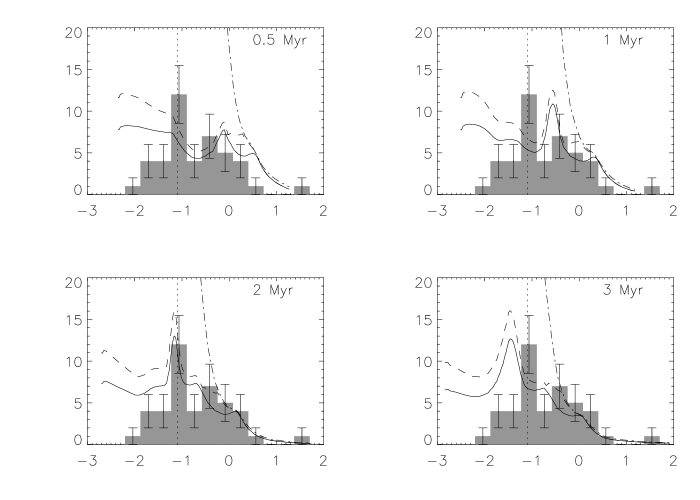
Figure 9: Synthetic LFs were calculated for 4 different ages of a coeval population on the basis of pre-main sequence tracks of D’Antona & Mazzitelli (1998) and 3 different underlying IMFs. The number of sources per bin is plotted vs. $\log L$, and the synthetic LFs are plotted over the observed LF for the Class II sources in Serpens (histogram). Both the Scalo (1998) three-segment power-law IMF (solid) and the Kroupa, Tout, Gilmore (1993) three-segment power-law IMF (dashed) seem plausible for a coeval population of $\sim$ 2 Myr all the way down to the estimated completeness limit at $L\sim 0.08L_{\odot}$ (dotted vertical line). The observed LF is also consistent with the Salpeter IMF (dashed-dotted) for this age at the high luminosity end (it has been extrapolated to low masses for reference only).

We have assumed coeval populations and three different underlying IMFs: the Salpeter IMF (Salpeter 1955), the Kroupa, Tout and Gilmore three-segment power-law IMF (Kroupa, Tout, Gilmore 1993), and the Scalo three-segment power-law IMF (Scalo 1998), hereafter S55, KTG93 and S98, respectively. With the IMF in the form: $dN/d\log M_{\star}\propto M_{\star}^{\alpha}$, the Salpeter IMF has one single index: $\alpha=-1.35$, originally determined for the mass interval 0.4 to 10 $M_{\odot}$ but in Fig. 9 extrapolated to lower masses for reference. Both the KTG93 and S98 IMFs have three different values of $\alpha$ for three (differently divided) segments. Bontemps et al. (2001) found for a large sample of Class II objects in $\rho$ Ophiuchi that the high mass end of the mass function was well fitted with the index $\alpha=-1.7$. Also, they found that the IMF starts to flatten at $M_{flat}=0.55M_{\odot}$ and stays “flat” down to $0.055M_{\odot}$ with a power-law index $\alpha_{flat}=-0.35$. These best fits of the two free parameters $M_{flat}$ and $\alpha_{flat}$ result in a mass function close to both the KTG93 and S98 IMFs for $\rho$ Ophiuchi.

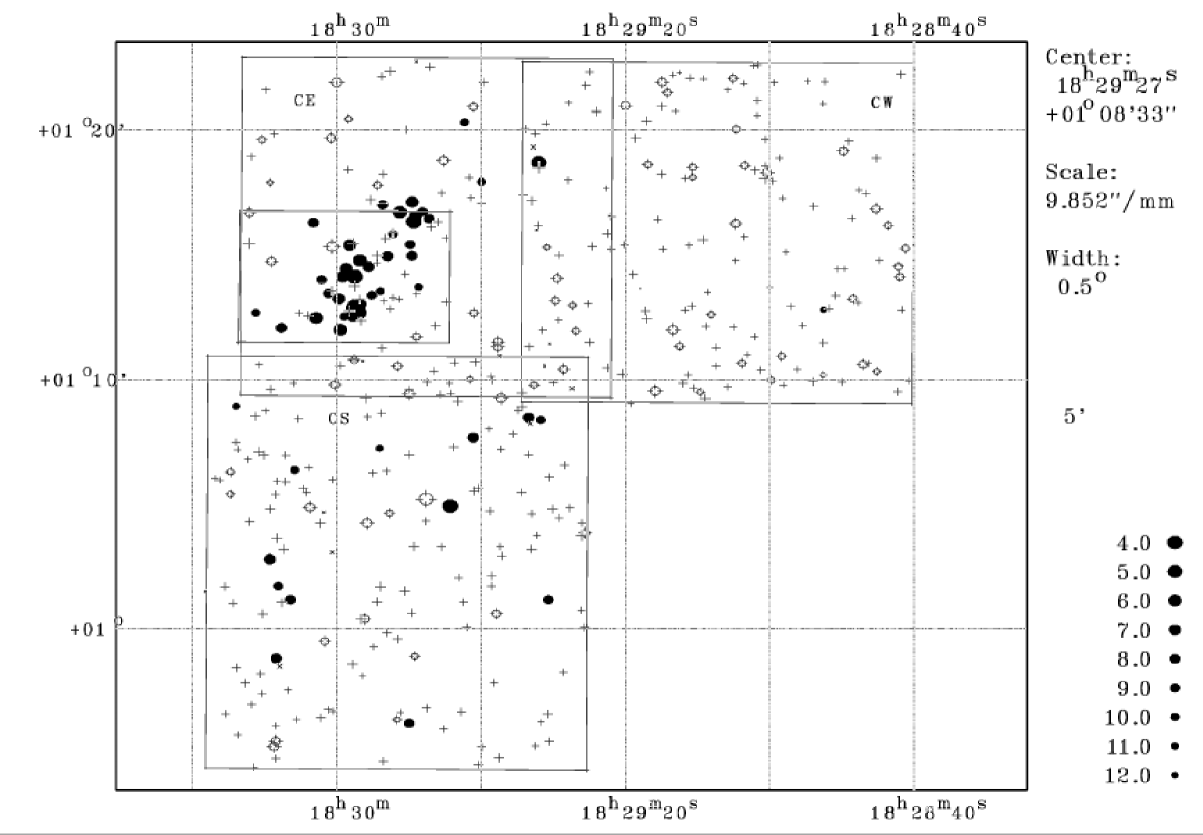
Figure 10: Spatial distribution of the ISOCAM sources in the Serpens Cloud. Sources with mid-IR excesses (filled circles) are seen to cluster strongly in the Cloud Core (field CE), while the CW field contains almost exclusively sources without mid-IR excesses (open circles). Indicated are also sources with 6.7 $\mu$m detections only (plus signs) and 14.3 $\mu$m detections only (crosses). The coordinates have epoch J2000. Each of the 3 separate ISOCAM rasters, CE, CW, and CS are indicated, and the small box outlines the region where deep JHK imaging is available (Kaas 1999a).

On the basis of the pre-main sequence evolutionary models of D’Antona & Mazzitelli (1994, 1998), with the 1998 upgrade for low mass stars, we have computed synthetic LFs for each IMF and for the four different ages: 0.5, 1, 2 and 3 Myr of a coeval cluster. Each window in Fig. 9 shows the result for one age, and the computed LFs are overplotted on the observed LF. The peak in the LF which wanders towards lower luminosities with increasing age arises because of the deuterium burning phase (Zinnecker, McCaughrean, Wilking 1993). Deuterium burning acts like a thermostat and hampers somewhat the contraction down the Hayashi track, causing a build-up of sources in a given luminosity bin for the case of coeval star formation. The peak in the observed LF, however, is approximately at the completeness limit of the sample, and we cannot put too much confidence in it. Nevertheless, it is obvious from the figure that the observed LF excludes ages of less than about 1 Myr for this Class II population for any of three underlying IMFs, which is in agreement with current understanding of YSO evolution. It is not possible to distinguish between the S98 IMF (solid line) and the KTG93 IMF (dashed), but both of them are plausible for a coeval population with an age of about 2 Myr, all the way down to the estimated completeness limit. Also the Salpeter IMF (dashed-dotted line) is in agreement with the observed LF for ages of 2-3 Myr at the high luminosity end. Its extrapolation to lower masses is given in the plots just for reference.

Note, however, that if star formation proceeds in a more continuous fashion, the structures in the model LFs will smooth out. We have checked the model LFs for the case of continuous star formation over several intervals from 0.5 to 3 Myrs. Although the statistics in the observed LF is poor, it seems we can exclude the combination of the above tested IMFs and continuous SF over periods of less than 2 Myrs. We also tested the case of a single star formation burst taking place 2 Myr ago but having various durations from 0.2 to 1.0 Myr. The peak in the observed LF is not secure enough to discriminate between the various burst durations. For the tested IMFs and SF histories, all we can conclude is that an age of less than 2 Myr for the Class II population seems implausible.

Corrections for binarity have not been applied, but such a correction would increase the populations in the lowest luminosity bins. We conclude that with the currently obtained LF the Class II mass function in Serpens is similar to the one in $\rho$ Ophiuchi (Bontemps et al. 2001), even though flat-spectrum sources were included in the $\rho$ Ophiuchi sample. We note that the typical stellar mass found for the Serpens Class II sample (i.e. the median) is 0.17 $M_{\odot}$, the same as in $\rho$ Ophiuchi (Bontemps et al. 2001). The total mass of the Class II sample in Serpens is $16.3M_{\odot}$.

We have also used the Baraffe et al. (1998) evolutionary tracks and calculated synthetic LFs with the same underlying IMFs as above and for the ages: 1, 2, 3, and 4 Myr. This model gives basically the same result as that of D’Antona & Mazzitelli (1998) for the degree of confidence we can put in our observed LF, taking the large error bars in the histogram into account.

Adopting the above deduced age of 2 Myr for the Serpens Class II population, our study is estimated to be complete to about $0.17M_{\odot}$, but to reach down to $0.03-0.04M_{\odot}$. Taking $0.08M_{\odot}$ as the border between low mass stars and brown dwarfs, we find 9 sub-stellar size objects in the Serpens Class II sample (those with $L_{\star}\leq 0.04L_{\odot}$ in Tab. 6). These are young brown dwarfs (BDs) apparently going through a Class II phase just like low mass stars. They all have IR excesses with no apparent deviations from other Class IIs in any aspect, which is consistent with the idea that they formed in the same way as low-mass stars do. Our sample of BDs is not complete, however, and we cannot discuss the frequency of occurrence of disks among BDs or set strong constraints on BD formation models.

Based on the age estimate above, we find that $\sim$ 21% of the Class II sample studied is made up of free-floating brown dwarfs. This is similar to the percentage found in $\rho$ Ophiuchi (Bontemps et al. 2001). The percentage in terms of mass is, however, only about 3% of the total mass for the whole Class II sample.

8 Spatial distributions

The spatial distribution of the ISOCAM sources is shown in Fig. 10 together with the location of the three main rasters CE, CW and CS. The filled circles indicate sources with mid-IR excesses (cf. Table 2), the open circles are the sources without mid-IR excesses (cf. Table 3), the plus signs are sources with 6.7 $\mu$m fluxes only, and crosses sources with 14.3 $\mu$m fluxes only. The small box outlines the $8\arcmin\times 6\arcmin$ field for which deep JHK imaging is obtained. The overall spatial distribution of the mid-IR excess YSOs shows a very clear concentration along a SE-NW oriented ridge within the CE field, mainly coinciding with what is known as the Serpens Cloud Core. In the CW field there is practically no sign of activity, while the distribution of IR-excess YSOs in the CS field is quite scattered. The majority of the mid-IR excess sources seem to be distributed along a curved filament pointing towards a centre of curvature around 18:29:10, +01:05:00 (J2000). Nothing particular was found at this location searching SIMBAD, however, and whether star formation along this arc may be externally triggered remains speculative. The IRAS Point Source Catalogue contains six sources in the area surveyed by ISOCAM (cf. Appendix A for details).

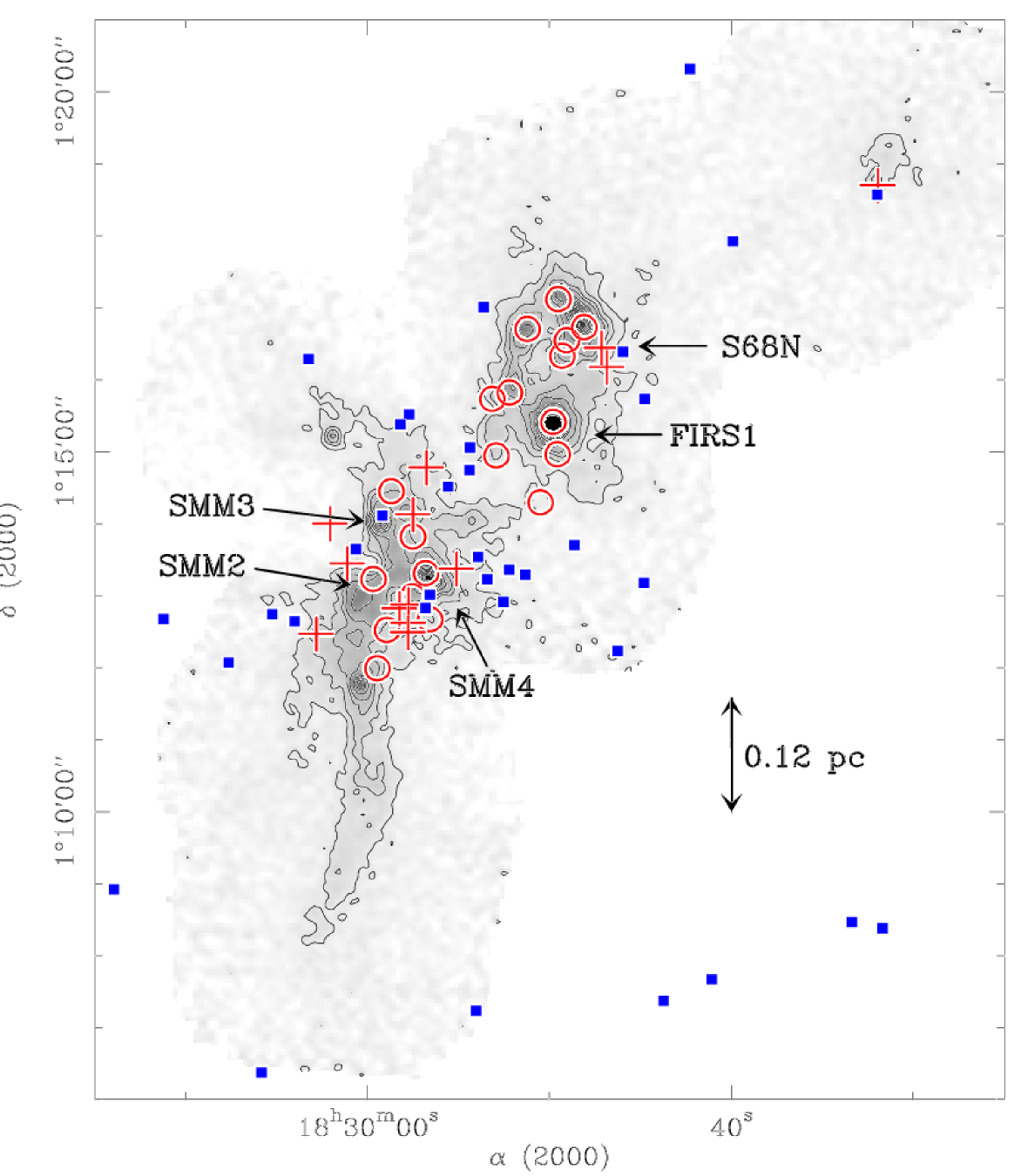
Figure 11: Dust continuum mosaic (contours and greyscale) of the Serpens main core taken at 1.3 mm with the IRAM 30m telescope and the MPIfR 37-channel bolometer array (MAMBO). Contour levels: 50. to 200 by 50, 300 to 1000. by 100. mJy/11″-beam; rms noise level: $\sim 17$ mJy/11″-beam. The Class 0 sources are indicated with names and arrows. The location of Class I sources (red circles), flat-spectrum sources (red crosses), and Class II sources (blue filled squares) demonstrates the strong clustering of protostar candidates along the dense filament.

Figure 12: A $K$ band image of the Serpens Cloud Core (6’ $\times$ 8’) from Kaas (1999a) with the Class Is (circles), flat-spectrum sources (squares) and Class IIs (hexagonals) marked. The “blue” ISOCAM sources are marked with triangles. The ridge along SE-NW is well outlined by the Class I and flat-spectrum sources.

8.1 Clustering scales

The concentration of young sources found along the NW-SE ridge, corresponds well to the pronounced density enhancement seen in the IRAM 1300 $\mu$m map in Fig. 11. It is evident that the Class I and the flat-spectrum sources are spatially more confined to the NW-SE ridge than the Class II sources, which have a more scattered distribution. In particular, the protostars seem to form a set of sub-clusters lined up along the ridge. These sub-clusters are in good positional agreement with the kinematically separated N₂H⁺ cores A,B,C,D found by Testi et al. (2000), especially with B,C, and D. The SVS4 sub-cluster lies between cores A and B, however, and is also displaced to the west of the SMM4 mm continuum peak.

Figure 13: The distribution of source separations for Class I and flat-spectrum objects (circles) and Class II sources (dots). The number of separations between sources (per bin) is plotted on the y-axis as a function of separation in arc minutes on the x-axis. The chosen bin size was 6 times the minimum separation, translating to 46.1$\arcsec$ and 66.1$\arcsec$ for the protostar and Class II source samples, respectively.

The spatial distribution of all the classes of YSOs within the central 6’ $\times$ 8’ of the Cloud Core can be seen overlaid on a $K$ band image in Fig. 12. To quantify the scale of sub-clustering of the two populations: protostar candidates (Class I and flat-spectrum sources) and Class II sources, we show for each population the distribution of separations between the sources. Figure 13 shows the result as the number of pairs vs. separation. The bin size was chosen to be 6 times the minimum separation. The difference between the two populations is clear. The protostar candidates (circles) have a minimum scale of clustering of about 0.12 pc (95$\arcsec$), a secondary peak at 0.36 pc, and practically no scattered distribution, while the Class II sources have a minimum clustering scale of about 0.25 pc, a secondary peak at 0.59 pc and a much more distributed population, in agreement with the maps. The clustering scale of 0.12 pc for the protostars agrees well with the range of radii of the N₂H⁺ cores: 0.055 to 0.115 pc (Olmi & Testi 2002), and the second peak at about 0.4 pc reflects well the size scale of the most active region in the Serpens Core.

The correspondence between the high density gas and the compactness of the protostar clusters indicates that these sources are found close to their birth place. Assuming a typical velocity dispersion in the range from 0.1 to 1 km s^-1, YSOs younger than $10^{5}$ yrs can be expected to have moved at most $0.1$ pc from their birth place. The typical ages of Class I sources are estimated to be of this order in other regions such as $\rho$ Ophiuchi (Greene et al. 1994) and Taurus (Kenyon et al. 1990). Our results indicate that the protostar candidates in each cluster must have formed from the same core at about the same time, which may put constraints on models of cloud fragmentation and core formation within clumps. Each sub-cluster contains between 6 and 12 protostar candidates, and this is just a lower limit because of the spatial resolution of ISOCAM. Adopting the Serpens distance of $260$ pc yields a protostar surface density in the sub-clusters in the range from 500-1100 pc^-2. To our knowledge, such a high spatial density of protostars has not been found in any other nearby star formation region, although we note that the Class 0 surface density in Orion-OMC3 is comparable to that in the Serpens Core (Chini et al. 1997).

The sub-clustering in the observed 2D projection of the cluster does not necessarily correspond to the true spatial distribution of the objects, but it seems highly unlikely that these concentrations are due to elongated cloud structures seen end-on. Sub-clustering was also found for the Class II sources in $\rho$ Ophiuchi (Bontemps et al. 2001), with a similar size scale as for the Class II population in Serpens. It seems likely that the strong clustering of Serpens protostars will evolve into looser clusters of Class IIs over a few 10⁶ yrs. The expansion of the clustering scales from 0.12 to 0.25 pc and the assumed ages of these two populations suggest that the velocity dispersion of the young stars is of the order of only 0.05 km s^-1.

9 Star formation rate and efficiency

Assuming that a recent burst of star formation took place $\sim 2\times$ 10⁵ yrs ago, producing the current population of protostars, we can derive a rough estimate of the star formation rate (SFR) and the star formation efficiency (SFE) in this burst. We use our sample of protostar candidates, the flat-spectrum and Class I sources found clustered along the NW-SE oriented ridge. We are not able to estimate their masses, but we hypothesize that they follow the same IMF as the Class II sample. Comparing the total mass of the Class II sample and correcting for the number of sources, we estimate a total mass of 12.1 $M_{\odot}$ for the protostar population. If these sources were formed gradually over $2\times$ 10⁵ yrs, the SFR in this microburst would be 6.1 $\times$ 10^-5 M_⊙/yr, or for typical masses of 0.17 M_⊙, one newborn star every $\sim$ 2800 yr. This SFR is significantly higher than the one found for the whole YSO population in $\rho$ Ophiuchi (Bontemps et al. 2001).

Comparing the protostellar masses with the gaseous mass in these cores will give us the star formation efficiency, defined as $SFE=M_{\rm star}/(M_{\rm star}+M_{\rm gas})$. According to Olmi & Testi (2002) the two sub-clumps they name NW and SE, which contain our four sub-clusters of protostars, are virialised with masses of 60 $M_{\odot}$ each. For our protostar candidates this yields a SFE of about 9 %. This is the local SFE for the sub-clusters along the NW-SE ridge. The global SFE calculated for the Class IIs and protostars over the entire cluster (i.e. 28.8 $M_{\odot}$ of stellar mass) is much lower. In the literature we find estimates of the total gas mass from 300 $M_{\odot}$ (McMullin et al. 2000) to 1500 $M_{\odot}$ (White et al. 1995) for surveyed areas of 5 to 10 arc minutes, which gives only upper limits on the SFE of the order of 2-9 %.

The above estimates are based on the hypothesis that the protostars follow the same IMF as the one found for the Class II sources. We have not attempted to derive the protostar mass function. Future high resolution far-IR observations (e.g. ESA’s Herschel Space Observatory) would be needed to yield bolometric luminosities of these clustered protostars, and with some assumptions on the accretion rates one could estimate their masses.

10 Summary and conclusions

We have used ISOCAM to survey 0.13 square degrees of the Serpens Cloud Core in two broad bands centred at 6.7 and 14.3 $\mu$m. In combination with our ground based deep $JHK$ imaging of the 48 square arcminute central region as well as additional $K$ band imaging of about 30 square arcminutes to the NW, and a 1.3 mm IRAM map of the central dense filament, we have investigated the mid-IR properties of the young stellar population. The following results are found:

• The number of point sources with reliable flux measurements are 392 at 6.7 $\mu$m and 139 at 14.3 $\mu$m. Of these, 124 are detected in both bands.

• On the basis of one single colour index, $[14.3/6.7]$, we found that 53 of the 124 objects possess strong mid-IR excesses. Only 28 of these were previously suggested YSO candidates. The large scale spatial distribution of these mid-IR excess sources is strongly concentrated towards the Cloud Core, where it is elongated along NW-SE.

• The near-IR $J-H/H-K$ diagram is found to have an efficiency of less than 50% in detecting IR excess sources. This efficieny is comparable to that one found in star formation regions in general from ISOCAM data (Kaas & Bontemps 2000) and $\rho$ Ophiuchi in particular (Bontemps et al. 2001) and should be kept in mind when interpreting $JHK$ based data in terms of disk fractions.

• The $H-K/K-m_{7}$ diagram separates well intrinsic IR excess from the effects of reddening. From this diagram we were able to increase the number of mid-IR excess sources to 70. This means a fractional increase in the investigated region by 25%.

• Combination of near-IR and mid-IR photometry for reddened stars without IR excesses enables us to estimate the extinction at 6.7 and 14.3 $\mu$m relative to that in the $K$ band in the Serpens direction. We find A₇ = 0.41 A_K and A₁₄ = 0.36 A_K. Our results agree with the extinction law measured towards the Galactic centre by Lutz et al. (1996), as well as with the results from the ISOGAL survey (Jiang et al. 2003).

• Classification of the Serpens YSOs in terms of the SED indices gives 20 Class I sources, 13 flat-spectrum sources, and 43 Class II sources. The number of Class I sources appears to be exceptionally large along the NW-SE oriented ridge, and the number fraction Class I/Class II is almost 10 times higher than normal, an indication that this part of the cluster is extremely young and active.

• The mid-IR luminosities of the Class I sources are on the average larger than those of the Class II sources. Since Class II sources are expected to have SEDs which peak approximately in the near and mid-IR, in contrast to Class Is which radiate most of their luminosity in the far-IR, we conclude that there is a weak indication of luminosity evolution in the Serpens Cloud Core.

• We have estimated extinction and stellar luminosities for the 43 Class II sources found in our survey. The Class II luminosity function is found to be compatible with co-eval formation about 2 Myrs ago and an underlying IMF of the three-segment power-law type (Kroupa, Tout, Gilmore 1993; Scalo 1998), similar to the mass function found in $\rho$ Ophiuchi (Bontemps et al. 2001). With this assumption on age, every fifth Class II is a young brown dwarf.

• Except for one case, the Class I sources are exclusively found in sub-clusters of sizes $\sim$ 0.12 pc distributed along the NW-SE oriented ridge. The sub-clusters also contain several flat-spectrum sources. In total, each core has formed between 6 and 12 protostars (lower limit) within a very short time. The spatial distribution of the Class II sources, on the other hand, is in general much more dispersed.

• On the assumption that the protostar candidates follow roughly the same IMF as the Class IIs, we derive a SFR of 6.1 $\times$ 10^-5 M_⊙/yr and a local SFE of 9% in the recent microburst of star formation forming the dense sub-clusters of protostars.

The results presented in this study show evidence that the sub-clusters in the central part of the Serpens Cloud Core were formed by a recent microburst of star formation. The extreme youth of this burst, deduced from the compact clusters of protostar candidates, is supported by independent investigations, such as the rich collection of Class 0 sources found by Casali et al. (1993) and Hurt & Barsony (1996) in the same regions. In addition to the clustered protostar population, we also find a more distributed population of Class II sources, for which we have deduced an age more or less typical of Class IIs found in other regions (2 Myr). In addition to these YSO generations, there is probably also a population of Class III sources, which is undistinguishable from the field star population in our study, but which should be looked for with proper search tools, such as e.g. X-ray mapping (Grosso et al. 2000).

Casali et al. (1993) suggested that their submm sources without near-IR counterparts represented a second phase of active star formation in Serpens. Here we show the co-existence of sources in the various evolutionary stages from Class II and flat-spectrum to Class I and Class 0 sources. While we find an age estimate of 2 Myr for the Class II population, it is highly unlikely that the clustered Class I and flat-spectrum sources are older than a few 10⁵ yrs. Our results therefore support the conclusions of Casali et al. (1993) that star formation has proceeded in several phases in Serpens.

Appendix A Notes on some individual sources

A.1 IRAS 18269+0116 (ISO-159, 160)

At the location of IRAS 18269+0116 we find ISO-159 and ISO-160, of which the latter is not detected at 14.3 $\mu$m. A $K$-band image shows that ISO-159 has a bow-shaped nebulosity 7$\arcsec$ to WNW (at a level of about 3-4 $\sigma$, see Fig. 4). The SED index classifies ISO-159 as a flat-spectrum source, while ISO-160 is either an extremely extinguished background source (analogous to CK2) or most likely a Class II object (cf Fig. 5).

A.2 IRAS 18271+0102 (ISO-221)

Identified as a YSO by Clark (1991) on the basis of its steeply rising SED towards longer wavelengths. With ISOCAM we see two very bright point sources (221 and 238), of which only ISO-221 has IR-excess.

A.3 EC21 (ISO-231)

This source was suggested as a YSO on the basis of its location in the $K$ vs $H-K$ diagram by Eiroa & Casali (1992). Deeper near-IR imaging detected the source also in the $J$ band, but found no near-IR excess (Kaas 1999a). It is located in the very dense and active S68N region, but whether it has intrinsic IR-excess at 7 $\mu$m or is only reddened (in that case, by 3 magnitudes in the $K$ band, which translates to $A_{V}\sim 30$ magnitudes), is not clear.

A.4 EC23 (ISO-232)

Proposed as a YSO on the basis of its $H-K$ colour and 3.08 $\mu$m ice feature (Eiroa & Casali 1992), but not found to have near-IR excess in a deeper JHK study (Kaas 1999a), nor mid-IR excess in this study.

A.5 IRAS 18272+0114 (DEOS, EC37, EC38, EC53, 234, 237, 241)

IRAS 18272+0114 is resolved into a cluster of protostar candidates: the Deeply Embedded Outburst Source (Hodapp et al. 1996), EC37, EC38 and EC53 (Eiroa & Casali 1992), and three new ISOCAM sources (234, 237, 241). ISO-241 is within the positional uncertainties associated with S68N, a radio source detected by McMullin et al. (1994) and found to satisfy the Class 0 criteria. We use the position at its 450 $\mu$m emission peak (Wolf-Chase et al. 1998). ISO-241 is a Class I, however, from the shape of its SED from 2 to 14 $\mu$m. Hodapp (1999) denotes the $K$-band source SMM9-IR, since it is located close to the SMM9 positions quoted in the literature (White et al. 1995; Wolf-Chase et al. 1998; Testi & Sargent 1998; Davis et al. 1999), and shows that it has a very faint $K$ companion about 2$\arcsec$ to the NE.

A.6 EC41 (ISO-258a) and FIRS1 (ISO-258b)

IRAS 18273+0113, also called FIRS1 and SMM1 (Rodriguez et al. 1989; Eiroa & Casali 1989; Casali et al. 1993), is associated with 5 mid-IR excess sources (EC41, 253, 270, 276, 277) plus one 14.3 $\mu$m source (258b).

ISO-Ser-258a is in agreement with the near-IR source positions of EC41 (Eiroa & Casali 1992) and GCNM23 (Giovannetti et al. 1998), and these are most likely the same source, a Class I YSO according to the $\alpha_{\rm IR}^{2-14}$ index. The ISOCAM source appeared slightly extended towards the SE both at 6.7 and 14.3 $\mu$m in most of our data. Larsson et al. (2000) found evidence for two separate sources, however, tracing pixel by pixel the 5 to 15 $\mu$m SED from CVF observations. This prompted us to take a more careful look, and we identified two clearly separated sources at 14.3 $\mu$m (rather than one extended source) in one of the deeper (and higher resolution) survey maps, D2 (cf. Fig. 14). The new source (called 258b), is located about 13$\arcsec$ to the SE of EC41. Since the radio position at RA(2000) = 18 29 49.73, DEC(2000) = 01 15 20.8 (Curiel et al. 1993) is 8.6$\arcsec$ to the west of 258b we find it unlikely that this source is the mid-IR counterpart of the far-IR source FIRS1, but it could be scattered light we see in the mid-IR. It is not entirely clear if this source is just a knot of the extended emission which appears to begin somewhat south of DEOS and is seen in both filters in Fig. 14. The northernmost part of this extended emission is, however, disturbed by a memory feature from the strong DEOS source in the raster scanning.

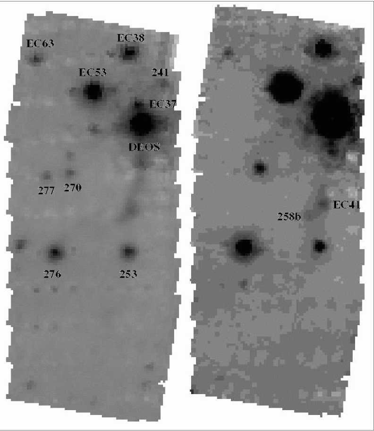
Figure 14: The deep map D2 at 6.7 $\mu$m (left) and 14.3 $\mu$m (right). North up and East left.

A.7 IRAS 18273+0059 (ISO-259)

A prominent extended emission seen in the ISOCAM images corresponds in position to IRAS 18273+0059 (Clark 1991). With ISOCAM, however, we see no apparent bright point source embedded in the nebulosity, but a moderately faint object is detected at 6.7 $\mu$m only. On optical plates the SE part of this extended emission is recognised as an optical reflection nebula.

A.8 IRAS 18274+0112

IRAS 18274+0112 is also composed of multiple mid-IR excess sources centred on SVS20 (cf. Fig 12). Higher spatial 25 $\mu$m resolution was obtained by Hurt & Barsony (1996), and their sources PS1 and PS2 (EC129) are among the bright mid-IR excess sources resolved with ISOCAM.

A.9 EC59 (ISO-272)

Included as a YSO candidate solely on the basis of its location in the $K$ vs $H-K$ diagram (Eiroa & Casali 1992), and no near-IR excess found in a deeper JHK study (Kaas 1999a). Since we have no indication of mid-IR excess its status remains inconclusive.

A.10 EC69 ISO-289

This source (also called CK10) was suggested as a YSO on the basis of its location in the $K$ vs $H-K$ diagram (Eiroa & Casali 1992), and while near-IR excess was found by Sogawa et al. (1997), no near-IR excess was found in a deeper JHK study (Kaas 1999a). The J-band magnitude has varied though: 15.7 in 1989, 14.96 in May 1992, 15.6 in Nov 1992, and 16.15 in Aug 1996 (Eiroa & Casali 1992; Sogawa et al. 1997; Giovannetti et al. 1998; Kaas 1999a). We conclude that it is a YSO, and with an $\alpha_{\rm IR}^{2-7}=-1.42$ it belongs in the Class II group.

A.11 EC95 & EC92 (ISO-317)

ISO-317 is located at the position of EC92 according to the coordinates given by Eiroa & Casali (1992), but the positional uncertainty is roughly $\pm 3\arcsec$. Also, the spatial resolution of ISOCAM is not sufficient to resolve the two neighbours EC92 and EC95, and it is likely that both are included in the ISOCAM fluxes. The mid-IR SED suggests a flat-spectrum source. Slightly closer to the position of EC95, but also with some positional uncertainty, Preibisch (1998) found an extremely strong X-ray source (Ser-X3).

A.12 ISO-331

This bright mid-IR source is detectable in $K$ as a nebulous spot only. Probably the $K$ flux is dominated by scattered light, and it is therefore not entirely correct to place ISO-331 in colour diagrams together with continuum sources. Nevertheless, the $K$ measurement gives a lower limit to the colour index of the object, which is classified as a Class I source. Its mid-IR position is about 25″to the NNW of SMM2 (Casali et al. 1993), and coincides roughly with the VLA 3.6 cm continuum source #11 found by Bontemps (1996).

A.13 CK2 (ISO-337)

According to ISOCAM data the source CK2, which is extremely red in the near-IR, has no mid-IR excess and can be interpreted as a background source, consistent with the suggestions of Churchwell & Koornneef (1986), Chiar et al. (1994), Casali & Eiroa (1996) and Sogawa et al. (1997). The extinction towards CK2 is high, A${}_{V}>$ 50 mag.