Statistical Significance of Small Scale Anisotropy in Arrival Directions of Ultra-High Energy Cosmic Rays

Abstract

Recently, the High Resolution Fly’s Eye (HiRes) experiment claims that there is no small scale anisotropy in the arrival distribution of ultra-high energy cosmic rays (UHECRs) above $E>10^{19}$ eV contrary to the Akeno Giant Air Shower Array (AGASA) observation. In this paper, we discuss the statistical significance of this discrepancy between the two experiments. We calculate arrival distribution of UHECRs above $10^{19}$ eV predicted by the source models constructed using the Optical Redshift Survey galaxy sample. We apply the new method developed by us for calculating arrival distribution in the presence of the galactic magnetic field. The great advantage of this method is that it enables us to calculate UHECR arrival distribution with lower energy ($\sim 10^{19}$ eV) than previous studies within reasonable time by following only the trajectories of UHECRs actually reaching the earth. It has been realized that the small scale anisotropy observed by the AGASA can be explained with the source number density $\sim 10^{-5\sim-6}$ Mpc^-3 assuming weak extragalactic magnetic field ($B\leq 1$ nG). We find that the predicted small scale anisotropy for this source number density is also consistent with the current HiRes data. We thus conclude that the statement by the HiRes experiment that they do not find small scale anisotropy in UHECR arrival distribution is not statistically significant at present. We also show future prospect of determining the source number density with increasing amount of observed data.

1 INTRODUCTION

The small scale anisotropy in the observed arrival distribution of ultra-high energy cosmic rays (UHECRs) is key in identifying their sources which will tell us a great deal about acceleration mechanisms, composition of UHECRs, and so on. The Akeno Giant Air Shower Array (AGASA) observation reveals the existence of the small scale clusterings in the isotropic arrival distribution of UHECRs (Takeda et al., 1999, 2001). The current AGASA data set of 57 events above 4 $\times 10^{19}$ eV contains four doublets and one triplet within a separation angle of 2.5^∘. Chance probability to observe such clusters under an isotropic distribution is only about 1 $\%$ (Hayashida et al., 2000; Takeda et al., 2001).

On the other hand, the recent claim by the High Resolution Fly’s Eye (HiRes; Wilkinson et al., 1999) experiment is that there is no small scale anisotropy in the UHECR arrival distribution above $E>10^{19}$ eV (162 events) which is observed by a stereo air fluorescence detector (Finley et al., 2003). The discrepancy between the AGASA and HiRes involves a number of consideration. Among them are the different numbers of the events, the possibility of the measured energies being shifted between the two experiments, (Marco, Blasi, & Olinto, 2003) and the different angular resolutions. The purpose of this paper is to discuss the first possibility. That is, we consider whether the discrepancy between the two experiments is statistically significant or not at present.

There is furthermore the contradiction on the presence or absence of the GZK cutoff (Greisen, 1966; Zatsepin & Kuz’min, 1966) in the cosmic-ray energy spectrum due to photopion production with the photons of the cosmic microwave background (CMB). The HiRes spectrum shows the GZK cutoff (Abu-Zayyad et al., 2002), but the AGASA spectrum does not (Takeda et al., 1998). The statistical significance of this discrepancy is already discussed in Marco, Blasi, & Olinto (2003) and shown to be low at present. This issue is left for future investigation by new large-aperture detectors under development, such as South and North Auger project (Capelle et al., 1998), the EUSO (Benson & Linsley, 1982), and the OWL (Cline & Stecker, 2000) experiments.

When we consider the statistical significance of the small scale anisotropy, we need to compare the observations with numerical calculations predicted by some kind of source distributions. In this paper, we use the Optical Redshift Survey (ORS; Santiago et al., 1995) galaxy sample to construct realistic source models of UHECRs. This sample has been adopted in our previous studies (Yoshiguchi et al., 2003a; Yoshiguchi, Nagataki, & Sato, 2003c, d). It has been realized that the small scale anisotropy well reflect the number density of UHECR sources (Yoshiguchi et al., 2003a; Yoshiguchi, Nagataki, & Sato, 2003c; Blasi & Marco, 2004). And also, it is shown that the small scale anisotropy above $E=4\times 10^{19}$ eV observed by the AGASA can be explained with the source number density $\sim 10^{-5\sim-6}$ assuming weak extragalactic magnetic field ($B\leq 1$ nG, EGMF) and that observed UHE particles are protons (Yoshiguchi et al., 2003a; Yoshiguchi, Nagataki, & Sato, 2003c; Blasi & Marco, 2004). We thus take the source number density as a parameter of our source model, and discuss the statistical significance of the small scale anisotropy by considering to what extent we can determine the source number density from the comparison of our model predictions with the HiRes observation.

As mentioned above, the claim by the HiRes experiment on the small scale anisotropy is based on the data of UHECR arrival directions above $10^{19}$ eV. UHE protons at such energies are significantly deflected by the galactic magnetic field (GMF) by a few $-\sim 10$ degrees. In order to accurately calculate the expected UHECR arrival distribution and compare with the observations, this effect should be taken into account.

In our recent work (Yoshiguchi, Nagataki, & Sato, 2003d), we presented a new method for calculating UHECR arrival distribution which can be applied to several source location scenarios including modifications by the GMF. Brief explanation of our method is as follows. We numerically calculate the propagation of anti-protons from the earth toward the outside of the Galaxy (we set a sphere centered around the Galactic center with radius $r_{\rm src}=$40 kpc as the boundary condition), considering the deflections due to the GMF. The anti-protons are ejected isotropically from the earth. By this calculation, we can obtain the trajectories and the sky map of position of anti-protons that have reached to the boundary at radius $r_{\rm src}=$ 40 kpc.

Next, we regard the obtained trajectories as the ones of PROTONs from the outside of the galaxy toward the earth. Also, we regard the obtained sky map of position of anti-proton at the boundary as relative probability distribution (per steradian) for PROTONs to be able to reach to the earth for the case in which the flux of the UHE protons from the extra-galactic region is isotropic (in this study, this flux corresponds to the one at the boundary $r_{\rm src}=40$ kpc). The validity of this treatment is supported by the Liouville’s theorem. When the flux of the UHE protons at the boundary is anisotropic (e.g., the source distribution is not isotropic), this effect can be included by multiplying this effect (that is, by multiplying the probability density of arrival direction of UHE protons from the extra-galactic region at the boundary) to the obtained relative probability density distribution mentioned above.

By adopting this new method, we can consider only the trajectories of protons which arrive to the earth, which, of course, helps us to save the CPU time efficiently and makes calculation of propagation of CRs even with low energies ($\sim 10^{19}$ eV) possible within a reasonable time.

With this method, we calculate the arrival distribution of UHE protons above $10^{19}$ eV for our source models. We also consider the energy loss processes when UHE protons propagate in the intergalactic space. Using the two point correlation function as statistical quantities for the small scale anisotropy, we compare our model prediction with the HiRes observation. We then discuss to what extent we can determine the source number density of UHECRs by the current HiRes data. We also briefly discuss future prospect of determining the source number density with the event number expected by future experiments.

In section 2, we introduce the GMF model. We explain the method for calculating UHECR arrival distribution in section 3. Results are shown in section 4. In section 5, we summarize the main results.

2 GALACTIC MAGNETIC FIELD

In this study, we adopt the GMF model used in Alvarez-Muniz, Engel & Stanev (2002); Yoshiguchi, Nagataki, & Sato (2003d, 2004), which is composed of the spiral and the dipole field. In the following, we briefly introduce this GMF model.

Faraday rotation measurements indicate that the GMF in the disk of the Galaxy has a spiral structure with field reversals at the optical Galactic arms (Beck, 2001). We use a bisymmetric spiral field (BSS) model, which is favored from recent work (Han, Manchester, & Qiao, 1999; Han, 2001). The Solar System is located at a distance $r_{||}=R_{\oplus}=8.5$ kpc from the center of the Galaxy in the Galactic plane. The local regular magnetic field in the vicinity of the Solar System is assumed to be $B_{\rm Solar}\sim 1.5~{}\mu{\rm G}$ in the direction $l=90^{\rm o}+p$ where the pitch angle is $p=-10^{\rm o}$ (Han & Qiao, 1994).

In the polar coordinates $(r_{||},\phi)$, the strength of the spiral field in the Galactic plane is given by

$$B(r_{||},\phi)=B_{0}~{}\left({R_{\oplus}\over r_{||}}\right)~{}\cos\left(\phi-\beta\ln{r_{||}\over r_{0}}\right)$$ (1)

where $B_{0}=4.4~{}\mu$G, $r_{0}=10.55$ kpc and $\beta=1/\tan p=-5.67$. The field decreases with Galactocentric distance as $1/r_{||}$ and it is zero for $r_{||}>20$ kpc. In the region around the Galactic center ($r_{||}<4$ kpc) the field is highly uncertain, and thus assumed to be constant and equal to its value at $r_{||}=4$ kpc.

The spiral field strengths above and below the Galactic plane are taken to decrease exponentially with two scale heights (Stanev, 1996)

$$|B(r_{||},\phi,z)|=|B(r_{||},\phi)|\left\{\begin{array}[]{lcl}\exp(-z):&|z|\leq 0.5~{}{\rm kpc}\\ \exp(\frac{-3}{8})~{}\exp(\frac{-z}{4}):&|z|>0.5~{}{\rm kpc}\end{array}\right.$$ (2)

where the factor $\exp(-3/8)$ makes the field continuous in $z$. The BSS spiral field we use is of even parity, that is, the field direction is preserved at disk crossing.

Observations show that the field in the Galactic halo is much weaker than that in the disk. In this work we assume that the regular field corresponds to a A0 dipole field as suggested in (Han, 2002). In spherical coordinates $(r,\theta,\varphi)$ the $(x,y,z)$ components of the halo field are given by:

$$B_{x}=-3~{}\mu_{\rm G}~{}{\sin\theta\cos\theta\cos\varphi}/r^{3}$$

$$B_{y}=-3~{}\mu_{\rm G}~{}{\sin\theta\cos\theta\sin\varphi}/r^{3}$$ (3)

$$B_{z}=\mu_{\rm G}~{}{(1-3\cos^{2}\theta)}/r^{3}~{}~{}~{}~{}~{}~{}~{}$$

where $\mu_{\rm G}\sim 184.2~{}{\rm\mu G~{}kpc^{3}}$ is the magnetic moment of the Galactic dipole. The dipole field is very strong in the central region of the Galaxy, but is only 0.3 $\mu$G in the vicinity of the Solar system, directed toward the North Galactic Pole.

There may be a significant turbulent component, $B_{\rm ran}$, of the Galactic magnetic field. Its field strength is difficult to measure and results found in literature are in the range of $B_{\rm ran}=0.5\dots 2B_{\rm reg}$ (Beck, 2001). However, we neglect the random field throughout the paper for simplicity. Possible dependence of the results on the assumption is discussed in the final section.

3 NUMERICAL METHOD

3.1 Propagation of UHE protons in the Intergalactic Space

The energy spectrum of UHECRs injected at extragalactic sources is modified by the energy loss processes when they propagate in the intergalactic space. In this subsection, we explain the method of Monte Carlo simulations for propagation of UHE protons in intergalactic space.

We assume that the composition of UHECRs are protons which are injected with a power law spectrum within the range of ($10^{19}$ - $10^{22}$)eV. We inject 10000 protons in each of 31 energy bins (10 bins per decade of energy). Then, UHE protons are propagated including the energy loss processes (explained below) over $3$ Gpc for $15$ Gyr. We take a power law index as 2.6 to fit the predicted energy spectrum to the one observed by the HiRes (Marco, Blasi, & Olinto, 2003).

UHE protons below $\sim 8\times 10^{19}$ eV lose their energies mainly by pair creations and adiabatic energy losses, and above it by photopion production (Berezinsky & Grigorieva, 1988; Yoshida & Teshima, 1993) in collisions with photons of the CMB. We treat the adiabatic loss as a continuous loss process. We calculate the redshift $z$ of source at a given distance using the cosmological parameters $H_{0}=71$ km s^-1 Mpc^-1, $\Omega_{m}=0.27$, and $\Omega_{\Lambda}=0.73$. Similarly, the pair production can be treated as a continuous loss process considering its small inelasticity ($\sim 10^{-3}$). We adopt the analytical fit functions given by Chodorowski, Zdziarske, & Sikora (1992) to calculate the energy loss rate for the pair production on isotropic photons.

On the other hand, protons lose a large fraction of their energy in the photopion production. For this reason, its treatment is very important. We use the interaction length and the energy distribution of final protons as a function of initial proton energy which is calculated by simulating the photopion production with the event generator SOPHIA (Mucke et al., 2000). The same approach has been adopted in our previous studies (Ide et al., 2001; Yoshiguchi et al., 2003a; Yoshiguchi, Nagataki, & Sato, 2003c, d).

In this study, we neglect the effect of the EGMF because of the following two reasons. First, numerical simulations of UHECR propagation in the EGMF including lower energy ($\sim 10^{19}$ eV) ones take a long CPU time. Secondly, we show in our previous study that small scale clustering observed by the AGASA can be well reproduced in the case of weak EGMF $(B<1{\rm nG})$ (Yoshiguchi et al., 2003a; Yoshiguchi, Nagataki, & Sato, 2003c). The purpose of this paper is to discuss whether the claim by the HiRes experiment is contrary to the AGASA result with statistical significance. We should calculate the arrival distribution of UHECRs in the situation that the AGASA experiment can be explained.

Of course, effects of strong EGMF (say, $\sim 100$ nG) on UHECR propagation are intensively investigated (Sigl, Miniati, & Ensslin, 2003, 2003b, 2004; Aloisio & Berezinsky, 2004), and can be hardly excluded considering the limited amount of observational data on the EGMF. However, we assume extremely weak EGMF throughout the paper.

3.2 Source Distribution

In this study, we apply the method for calculating the UHECR arrival distribution with modifications by the GMF (section 3.3) to our source location scenario, which is constructed by using the ORS (Santiago et al., 1995) galaxy catalog.

In order to calculate the distribution of arrival directions of UHECRs realistically, there are two key elements of the galaxy sample to be corrected. First, galaxies in a given magnitude-limited sample are biased tracers of matter distribution because of the flux limit (Yoshiguchi et al., 2003b). Although the sample of galaxies more luminous than $-20.5$ mag is complete within 80 $h^{-1}$ Mpc (where $h$ is the Hubble constant divided by 100 km s^-1 and we use $h=0.71$), it does not contain galaxies outside it for the reason of the selection effect. We distribute sources of UHECRs outside 80 $h^{-1}$ Mpc homogeneously. Their number density is set to be equal to that inside 80 $h^{-1}$ Mpc.

Secondly, our ORS sample does not include galaxies in the zone of avoidance ($|b|<20^{\circ}$). In the same way, we distribute UHECR sources in this region homogeneously, and calculate its number density from the number of galaxies in the observed region.

As mentioned above, we take the number density of UHECR sources as our model parameter when we construct the source models. For a given number density, we randomly select galaxies from the above sample with probability proportional to the absolute luminosity of each galaxy. In this paper, the model parameters are taken to be $10^{-3}$, $10^{-4}$, $10^{-5}$, and $10^{-6}$ Mpc^-3.

3.3 Calculation of the UHECR Arrival Distribution with modifications by the GMF

This subsection provides the method of calculation of UHECR arrival distribution with modifications by the GMF. The explanations largely follows our recent paper (Yoshiguchi, Nagataki, & Sato, 2003d). We start by injecting anti-protons from the earth isotropically, and follow each trajectory until

1. anti-proton reaches a sphere of radius $40$ kpc centered at the galactic center, or

2. the total path length traveled by anti-proton is larger than $200$ kpc,

by integrating the equations of motion in the magnetic field. It is noted that we regard these anti-protons as PROTONs injected from the outside of the Galaxy toward the earth. The number of propagated anti-proton is 2,000,000. We have checked that the number of trajectories which are stopped by the limit (2) is smaller than $0.1$% of the total number. The energy loss of protons can be neglected for these distances. Accordingly, we inject anti-protons with injection spectrum similar to the observed one $\sim E^{-2.7}$. (Note that this is not the energy spectrum injected at extragalactic sources.)

The result of the velocity directions of anti-protons at the sphere of radius $40$ kpc is shown in the right panel of figure 1 in the galactic coordinate. From Liouville’s theorem, if the cosmic-ray flux outside the Galaxy is isotropic, one expects an isotropic flux at the earth even in the presence of the GMF. This theorem is confirmed by numerical calculations shown in figure 6 of Alvarez-Muniz, Engel & Stanev (2002), which is the same figure as our figure 1 except for threshold energy. Thus, the mapping of the velocity directions in the right panel of figure 1 corresponds to the sources which actually give rise to the flux at the earth in the case that the sources (including ones which do not actually give rise to the flux at the earth) are distributed uniformly.

Figure 1: Arrival directions of anti-protons with $E>10^{19.0}$ eV at the sphere of Galactocentric radius of $40$ kpc (right panel) in the galactic coordinate. The anti-protons are injected at the earth isotropically (as shown in the left panel) with an injection spectrum $E^{-2.7}$.

We calculate the UHECR arrival distribution for our source scenario using the numerical data of the propagation of UHE anti-protons in the Galaxy. Detailed method is as follows. At first, we divide the sky into a number of bins with the same solid angle. The number of bins is taken to be $360(l)\times 200(b)$. We then distribute all the trajectories into each bin according to their directions of velocities (source directions) at the sphere of radius $40$ kpc. Finally, we randomly select trajectories from each bin with probability $P_{\rm selec}(j,k,E)$ defined as

$$P_{\rm selec}(j,k,E)\propto\sum_{i}\frac{1}{d_{i}^{2}}\,\frac{dN/dE(d_{i},E)}{E^{-2.7}}.$$ (4)

Here subscripts j and k distinguish each cell of the sky, $d_{i}$ is distance of each galaxy within the cell of (j,k), and the summation runs over all of the galaxies within it. $E$ is the energy of proton, and $dN/dE(d_{i},E)$ is the energy spectrum of protons at our galaxy injected at a source of distance $d_{i}$.

The normalization of $P_{\rm selec}(j,k,E)$ is determined so as to set the total number of events equal to a given number, for example, the event number of the current HiRes data. When $P_{\rm selec}>1$, we newly generate events with number of $(P_{\rm selec}-1)\times N(j,k)$, where $N(j,k)$ is the number of trajectories within the sky cell of $(j,k)$. The arrival angle of newly generated proton (equivalently, injection angle of anti-proton) at the earth is calculated by adding a normally distributed deviate with zero mean and variance equal to the experimental resolution $2.8^{\circ}$ $(1.8^{\circ})$ for $E>10^{19}$ eV $(4\times 10^{19}{\rm eV})$ to the original arrival angle.

3.4 Statistical Methods

A standard tool for searching the small scale anisotropy is the two point correlation function. This subsection provides the explanation of this function.

We start from a set of simulated events. For each event, we divide the sphere into concentric bins of angular size $\Delta\theta$, and count the number of events falling into each bin. We then divide it by the solid angle of the corresponding bin, that is,

$$N(\theta)=\frac{1}{2\pi|\cos\theta-\cos(\theta+\Delta\theta)|}\sum_{\theta\leq\phi\leq\theta+\Delta\theta}1\;\;\;[\rm sr^{-1}],$$ (5)

where $\phi$ denotes the separation angle of the two events. $\Delta\theta$ is taken to be $2^{\circ}$ in this analysis. We also evaluate $N_{\rm uni}(\theta)$ for an equal number of events simulated in a Monte Carlo for uniform source distribution. The estimator for the correlation function is then defined as $w(\theta)=N(\theta)/N_{\rm uni}(\theta)-1$.

The two point correlation function of the HiRes data with 164 events above $10^{19}$ eV do not show significant small scale anisotropy, and is consistent with isotropic source distribution within $1\sigma$ confidence level. We thus compare the two point correlation functions predicted by our source models with that expected for isotropic source distribution rather than the HiRes data itself. When we consider to what extent we can determine the source number density of UHECRs, we have to quantify deviations of predictions by our source models from isotropic sources. To do so, we define the variable $\chi^{2}$ as

$$\chi^{2}=\frac{1}{N_{\rm bin}}\sum_{i=1}^{i=N_{\rm bin}}\frac{(w_{\rm th}(\theta_{\rm i})-w_{\rm uni}(\theta_{i}))^{2}}{(\sigma_{\rm i}^{\rm th})^{2}+(\sigma_{\rm i}^{\rm uni})^{2}},$$ (6)

where $\theta_{\rm i}$ is the angle at i-th bin. $\sigma_{\rm i}^{\rm th}$ and $\sigma_{\rm i}^{\rm uni}$ are the statistical fluctuations of $w_{\rm th}$ and $w_{\rm uni}$ at the angle $\theta_{\rm i}$. The summation is taken over the angular bins, whose number is denoted by $N_{\rm bin}$.

Even if we specify the source number density, source distribution itself can not be determined because of randomness when we select galaxies from the ORS sample. Therefore, we first evaluate $\chi^{2}$ for a source distribution in the case of a given number density of UHECR sources. We then repeat such calculations for a number of realizations of the source selection, and obtain the probability distribution of $\chi^{2}$ for a source number density. The source selections are performed 100 times for all the source number densities.

4 RESULTS

4.1 Arrival Distribution of UHECRs

In this subsection, we present the results of arrival distribution of UHECRs above $10^{19}$ eV obtained by using the method explained in section 3.3. Figure 2 and 3 show realizations of the event generations in the case of the source number density $10^{-3}$ and $10^{-5}$ Mpc^-3, respectively. The events are shown by color according to their energies. Note that the event number of HiRes data is 162 ($E>10^{19}$ eV). This roughly corresponds to 300 events of figure 2 and 3, considering the difference of the range $\delta$ (declination) between the observation and numerical calculation.

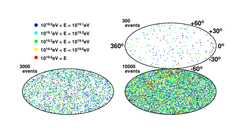
Figure 2: Arrival directions of protons with $E>10^{19}$ eV predicted by a source distribution for the source number density $10^{-3}$ Mpc^-3 in Galactic coordinates. Events are shown by color according to their energies.

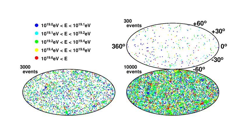
Figure 3: Same as figure 2, but for the source number density $10^{-5}$ Mpc^-3.

As is evident from figure 2 and 3, arrival distributions of UHECRs are quite isotropic. The harmonic analysis to the right ascension distribution of events is the conventional method to search for global anisotropy of cosmic ray arrival distribution. Using this analysis, we have checked that large scale isotropy predicted by our source models is consistent with isotropic source distribution within a 90$\%$ confidence level with event number equal to the current HiRes and AGASA observations. On the other hand, arrival distributions observed by the HiRes and AGASA do not also show any significant global anisotropy. There is no discrepancy between the two experiments. Thus we do not discuss large scale isotropy in the following.

Comparing figure 2 and 3, we easily find that arrival distribution expected for smaller source number density exhibits stronger anisotropy on small angle scale. This is simply because contributions from each source to the total events are larger for smaller source number density. Furthermore, the clustered events are aligned in the sky according to the order of their energies, reflecting the direction of the GMF at each direction. This interesting feature becomes evident with increasing amount of the event number.

4.2 Statistical significance of the small scale anisotropy

Next, we discuss the statistics on arrival distribution of UHECRs. Figure 4.2 and 4.2 show the two point correlation function expected in the case of source distributions of figure 2 and 3, respectively. We calculate the two point correlation function for the simulated events within only $0^{\circ}\leq\delta\leq 90^{\circ}$ in accordance with the HiRes exposure. For this reason, the event numbers written in figure 4.2 and 4.2 differ from the ones in figure 2 and 3. The error bars represent 1 $\sigma$ statistical fluctuations of our numerical calculations due to the finite number of events. The shaded regions represent 1 $\sigma$ fluctuations for uniform source distribution. The event selections are performed $1000$, $100$, and $30$ times for the event number $150$, $1500$, and $5000$, respectively. It is noted that we compare our numerical results with not the HiRes data itself but the prediction of uniform source distribution. We do not have to consider the non-uniform observation in the angular sky.

Two point correlation function predicted by a realization of the source selection for the number density $10^{-3}$ Mpc^-3. We calculate the two point correlation function for the simulated events within only $0^{\circ}\leq\delta\leq 90^{\circ}$ in accordance with the HiRes exposure. The error bars represent 1 $\sigma$ statistical fluctuations due to the finite number of events for our numerical calculations. The shaded regions represent 1 $\sigma$ fluctuations for uniform source distribution. The event selections are performed $1000$, $100$, and $30$ times for the event number $150$, $1500$, and $5000$, respectively.

As mentioned before, it is evident that smaller source number density predicts stronger correlation between events at small angle scale. The small scale anisotropy well reflects the number density of UHECR sources. It is already shown that the small scale anisotropy above $E=4\times 10^{19}$ eV observed by the AGASA can be explained with the source number density $\sim 10^{-5\sim-6}$ Mpc ^-3 assuming weak extragalactic magnetic field ($B\leq 1$ nG, EGMF) (Yoshiguchi et al., 2003a; Yoshiguchi, Nagataki, & Sato, 2003c; Blasi & Marco, 2004). We thus discuss the statistical significance of the discrepancy between the HiRes and AGASA by considering to what extent we can determine the UHECR source number density from the current HiRes data.

Even if we specify the source number density, source distribution itself can not be determined because of randomness when we select galaxies from the ORS sample. Therefore, we first evaluate the statistical significance of deviation of the two point correlation function predicted by a source distribution for a given number density from that expected for uniform source distribution. We then repeat such calculations for a number of realizations of the source selection, and obtain the probability distribution of $\chi^{2}$ for a given source number density.

Same as figure 4.2, but for the number density $10^{-5}$ Mpc^-3.

Probability distribution of statistical significance of deviation of our model prediction from that of isotropic sources ($\chi^{2}$) when the source selection from our ORS sample is performed 100 times. The data of the two point correlation at the smallest angle are used ($N_{\rm bin}=1$).

The results of the probability distribution of $\chi^{2}$ for $N_{\rm bin}=1$ and $5$ are shown as histograms in figure 4.2 and 4.2, respectively. The source selection is performed 100 times for all the source number densities. As we can see from the figures, differences between probability distributions of $\chi^{2}$ for different source number densities are clearer when $N_{\rm bin}=1$. This is related to the fact that the two point correlation function is most sensitive to the source number density at the smallest angular bin (see, figure 4.2 and 4.2). We thus focus our attention to the result for $N_{\rm bin}=1$ in the following.

Same as figure 4.2, but for $N_{\rm bin}=5$.

As mentioned, we know that the small scale anisotropy observed by the AGASA can be explained with the number density $\sim 10^{-6\sim-5}$ Mpc^-3. From figure 4.2, it is found that the small scale anisotropy predicted by this source number density is also consistent with the prediction of isotropic source distribution when the event number is equal to the HiRes data ($\sim 150$). It is noted that the AGASA data have about 1000 events above $10^{19}$ eV. The possibility that the number density is about $\sim 10^{-6\sim-5}$ Mpc^-3 can not be ruled out, although the HiRes result seems to be in agreement with the isotropic source distribution. We thus conclude that the statement by the HiRes experiment that they do not find small scale anisotropy in UHECR arrival distribution is not statistically significant at present.

We now turn to the future prospects of determining the UHECR source number density. The probability distributions of $\chi^{2}$ with larger event number than the current observations are also shown in figure 4.2. Of course, there is no observational data to be compared. We thus compare the model predictions with the case of isotropic source distribution. The results should be interpreted as quantifying deviations of our calculations from the prediction of isotropic sources in the unit of statistical fluctuations.

As is evident from figure 4.2, difference between the probability distribution of $\chi^{2}$ for different source number densities become clear when the number of data increases. We will be able to determine the source number density by the future observations of the small scale anisotropy. In order to discuss to what accuracy we can know the source number density, we need to calculate the probability distribution of $\chi^{2}$ more precisely with a large number of simulations of the source selection. This issue is beyond the scope of the present paper. We will study it in a future publication.

5 SUMMARY AND DISCUSSION

In this paper, we considered the statistical significance of the discrepancy between the HiRes and the AGASA experiment on the small scale anisotropy in arrival distribution of UHECRs. We calculated arrival distribution of UHECRs above $10^{19}$ eV predicted by our source models constructed using the ORS galaxy sample. We applied the new method developed by us (Yoshiguchi, Nagataki, & Sato, 2003d) for calculating arrival distribution with the modifications by the GMF. The great advantage of this method is that it enables us to calculate UHECR arrival distribution with lower energy ($\sim 10^{19}$ eV) than previous studies by following only the trajectories actually reaching the earth.

It has been realized that the small scale anisotropy in the UHECR arrival distribution well reflects the number density of UHECR sources (Yoshiguchi et al., 2003a; Yoshiguchi, Nagataki, & Sato, 2003c; Blasi & Marco, 2004). And also, it is shown that the small scale anisotropy above $E=4\times 10^{19}$ eV observed by the AGASA can be explained with the source number density $\sim 10^{-5\sim-6}$ assuming weak extragalactic magnetic field ($B\leq 1$ nG, EGMF) and that observed UHE particles are protons (Yoshiguchi et al., 2003a; Yoshiguchi, Nagataki, & Sato, 2003c; Blasi & Marco, 2004). We thus took the source number density as a parameter of our source model, and discussed the statistical significance of the small scale anisotropy by considering to what extent we can determine the source number density from the comparison of the model predictions with the HiRes observation.

When we consider to what extent we can determine the source number density of UHECRs, we have to quantify deviations of predictions by our source models from the observation. And also, even if we specify the source number density of our model, source distribution itself can not be determined because of randomness when we select galaxies from the ORS sample. Therefore, we first evaluated the statistical significance of deviation ($\chi^{2}$) of the two point correlation function predicted by a source distribution for a given number density from that expected for uniform source distribution. We then repeated such calculations for a number of realizations of the source selection. This gave the probability distributions of $\chi^{2}$ for various number densities of UHECR sources.

The results for $N_{\rm bin}=1$ and $5$ show that differences between probability distributions of $\chi^{2}$ for different source number densities are clearer when $N_{\rm bin}=1$. This is related to the fact that the two point correlation function is most sensitive to the source number density at the smallest angular bin. We thus focused our attention to the result of $N_{\rm bin}=1$. As mentioned above, we know that the small scale anisotropy observed by the AGASA can be explained with the number density $\sim 10^{-6\sim-5}$ Mpc^-3. It is found that the small scale anisotropy predicted by this source number density is also consistent with the prediction of isotropic source distribution when the event number is equal to the HiRes data ($\sim 150$). Note that the data number of AGASA is about $1000$ above $10^{19}$ eV. The possibility that the number density is about $\sim 10^{-6\sim-5}$ Mpc^-3 can not be ruled out, although the HiRes result seems to be in agreement with the isotropic source distribution. We thus concluded that the statement by the HiRes experiment that they do not find small scale anisotropy in UHECR arrival distribution is not statistically significant at present.

We also discussed the future prospects of determining the UHECR source number density. As is evident from figure 4.2, difference between the probability distribution of $\chi^{2}$ for different source number densities become clear when the number of data increases. We will be able to determine the source number density by the future observations of the small scale anisotropy. In order to discuss to what accuracy we can know the source number density, we need to calculate the probability distribution of $\chi^{2}$ more precisely with a large number of simulations of the source selection. This issue deserves further investigation.

Finally, we mention the assumptions made in this paper. We neglected the effects of the extragalactic magnetic field and the random component of the GMF. If we take these effect into account, the small scale anisotropy obtained by numerical calculations become less obvious. In this case, our statement that the small scale anisotropy for $\sim 10^{-5\sim-6}$ Mpc^-3 is also consistent with the prediction of isotropic sources when the event number is equal to the HiRes data ($\sim 150$) remains to be valid. Hence, the assumptions are not so important for our conclusion.

Note added: While we are finishing this study, a paper by the HiRes collaboration (Abbasi et al., 2004) appears on the net, where they present the results of a search for small scale anisotropy in the observed arrival distribution of UHECRs. They find no small scale anisotropy in 271 events above $10^{19}$ eV, which is slightly larger than the event number considered in the present study (164). However, this increase of the event number will not affect our conclusion very much, as seen from figure 4.2.

References

- Abu-Zayyad et al. (2002) Abu-Zayyad T. et al. (The HiRes Collaboration) 2002, astro-ph/0208243
- Abbasi et al. (2004) Abbasi R.U. et al. (The HiRes Collaboration) 2004, astro-ph/0404137
- Alvarez-Muniz, Engel & Stanev (2002) Alvarez-Muniz J., Engel R., & Stanev T. 2002, ApJ, 572, 185
- Beck (2001) Beck R. 2001, Space. Sci. Rev. 99, 243
- Benson & Linsley (1982) Benson R., & Linsley J. 1982, A&A, 7, 161
- Berezinsky & Grigorieva (1988) Berezinsky V., & Grigorieva S.I. 1988, A&A, 199, 1
- Aloisio & Berezinsky (2004) Aloisio R., & Berezinsky V. 2004, astro-ph/0403095
- Bird et al. (1994) Bird D.J., et al. 1994, ApJ, 424, 491
- Blasi & Marco (2004) Blasi P., & Marco D.D. 2004, Astropart. Phys., 20, 559
- Capelle et al. (1998) Capelle K.S., Cronin J.W., & Parente G., Zas E. 1998, APh, 8, 321
- Chodorowski, Zdziarske, & Sikora (1992) Chodorowski M.J., Zdziarske A.A., & Sikora M. 1992, ApJ, 400, 181
- Cline & Stecker (2000) Cline D.B., & Stecker F.W. OWL/AirWatch science white paper, astro-ph/0003459
- Finley et al. (2003) Finley C.B., Westerhoff S., for the HiRes Collaboration 2003, Proceeding of 28th ICRC, 433
- Greisen (1966) Greisen K. 1966, Phys. Rev. Lett., 16, 748
- Han & Qiao (1994) Han J.L., & Qiao G.J. 1994, A&A, 288, 759
- Han, Manchester, & Qiao (1999) Han J.L., Manchester R.N., & Qiao G.J. 1999, MNRAS, 306, 371
- Han (2001) Han J.L., 2001, Ap&SS, 278, 181
- Han (2002) Han J.L., 2002, astro-ph/0110319.
- Hayashida et al. (1999) Hayashida N., et al. 1999 APh, 10, 303
- Hayashida et al. (2000) Hayashida N., et al. 2000, astro-ph/0008102
- Ide et al. (2001) Ide Y., Nagataki S., Tsubaki S., Yoshiguchi H., & Sato K. 2001, PASJ, 53, 1153
- Isola & Sigl (2002) Isola C., & Sigl G. 2002, astro-ph/0203273
- Marco, Blasi, & Olinto (2003) Marco D.D., Blasi P., & Olinto A.V. 2003, astro-ph/0301497
- Mucke et al. (2000) Mucke A., Engel R., Rachen J.P., Protheroe R.J., & Stanev T. 2000, Comput. Phys. Commun. 124, 290
- Santiago et al. (1995) Santiago B.X., Strauss M.A., Lahav O., Davis M., Dressler A., & Huchra J.P. 1995, ApJ, 446, 457
- Sigl, Miniati, & Ensslin (2003) Sigl G., Miniati F., & Ensslin T.A. 2003, astro-ph/0302388
- Sigl, Miniati, & Ensslin (2003b) Sigl G., Miniati F., & Ensslin T.A. 2003, astro-ph/0309695
- Sigl, Miniati, & Ensslin (2004) Sigl G., Miniati F., & Ensslin T.A. 2004, astro-ph/0401084
- Stanev (1996) Stanev T. 1996, ApJ, 479, 290
- Takeda et al. (1998) Takeda M., et al. 1998, Phys. Rev. Lett., 81, 1163
- Takeda et al. (1999) Takeda M., et al. 1999, ApJ, 522, 225
- Takeda et al. (2001) Takeda M., et al. 2001, Proceeding of ICRC 2001, 341
- Wilkinson et al. (1999) Wilkinson C.R., et al. 1999, APh, 12, 121
- Yoshida & Teshima (1993) Yoshida S., & Teshima M. 1993, Prog. Theor. Phys. 89, 833
- Yoshida et al. (1995) Yoshida S., et al. 1995 Astropart. Phys., 3, 105
- Yoshiguchi et al. (2003a) Yoshiguchi H., Nagataki S., Tsubaki S., & Sato K. 2003a, ApJ, 586, 1211
- Yoshiguchi et al. (2003b) Yoshiguchi H., Nagataki S., Sato K., Ohama N., & Okamura S. 2003b, PASJ, 55, 121 (astro-ph/0212061)
- Yoshiguchi, Nagataki, & Sato (2003c) Yoshiguchi H., Nagataki S., Sato K. 2003c, ApJ, 592, 311
- Yoshiguchi, Nagataki, & Sato (2003d) Yoshiguchi H., Nagataki S., Sato K. 2003d, ApJ, 596, 1044
- Yoshiguchi, Nagataki, & Sato (2004) Yoshiguchi H., Nagataki S., Sato K. 2004, ApJ, in press
- Zatsepin & Kuz’min (1966) Zatsepin G.T., & Kuz’min V.A. 1966, JETP Lett., 4, 78