Theoretical isochrones in several photometric systems

Following Paper I, we provide extended tables of bolometric corrections, extinction coefficients, stellar isochrones, and integrated magnitudes and colours of single-burst stellar populations, for the Sloan Digital Sky Survey (SDSS) $ugriz$ photometric system. They are tested on comparisons with DR1 data for a few stellar systems, namely the Palomar 5 and NGC 2419 globular clusters and the Draco dSph galaxy.

1 Introduction

The Sloan Digital Sky Survey (SDSS; see York et al. 2000) is one of the most impressive astronomical campaigns ever carried out. It aims at providing photometry and subsequent spectroscopy for objects covering about one quarter of the entire sky. SDSS photometry is being obtained near-simultaneously in five broad-band filters in drift-scan mode, which results in highly homogeneous data. The effective exposure time for imaging is approximately 54 s with a limiting magnitude of $r\sim 22.6$. The primary science goals of the SDSS are at extragalactic and cosmological studies such as galaxy evolution as a function of redshift (e.g., Gómez et al. 2003; Eisenstein et al. 2003; Blanton et al. 2001), the search for high-redshift quasars (e.g., Fan et al. 2001, 2003), weak lensing (e.g., Fischer et al. 2000; McKay et al. 2002), and the large-scale structure distribution of galaxies (e.g., Dodelson et al. 2002; Zehavi et al. 2002). However, the SDSS also provides a huge database for various areas of stellar and Galactic astronomy, e.g., the search for rare or special stellar objects (e.g., Margon et al. 2002; Hawley et al. 2002; Helmi et al. 2003), the study of resolved star clusters and nearby Milky Way satellites (e.g., Odenkirchen et al. 2001a,b), and studies of Milky Way substructure (e.g., Chen et al. 2001; Newberg et al. 2002; Yanny et al. 2003). For an overview of SDSS science, see Grebel (2001). Our paper aims at providing tools for the interpretation of SDSS stellar photometry data, i.e., isochrones transformed to the SDSS photometric system.

The SDSS began regular operations in 2000 and will run until 2005. The SDSS data products include images in five passbands, photometrically and astrometrically calibrated object catalogs with a wealth of information on the properties of the recorded objects, and wavelength- and flux-calibrated spectra with redshifts. An Early Data Release (EDR) of SDSS commissioning data occurred in July 2001 (Stoughton et al. 2002), and Data Release 1 (DR1) took place in May 2003 (DR1; Abazajian et al. 2003). The currently publicly available SDSS photometry data cover 2099 square degrees, about one fifth of the total anticipated survey area. The subsequent data releases are planned to occur on a yearly basis. The final one is scheduled for 2006. It is estimated that the SDSS will ultimately comprise some $8\cdot 10^{7}$ stars with high-quality five-band photometry, including Galactic halo and disk field stars, stars in globular clusters, and in nearby resolved dwarf galaxies.

The SDSS has designed, defined, and calibrated its own photometric system (Fukugita et al. 1996; Gunn et al. 1998; Smith et al. 2003), which is characterized by the following particularities: (1) the use of a modified Thuan-Gunn broadband filter system called $ugriz$; (2) a zero-point definition in the AB magnitude system; (3) the use of a modified, non-logarithmic, definition of the magnitude scale (Lupton, Gunn, & Szalay 1999). As a consequence, SDSS photometry cannot be easily transformed into traditional systems, or at least any transformation is likely to lead to a significant loss of the photometric information contained in SDSS data of fainter sources. This presents a problem not only for users of the SDSS databases, but also for astronomers who obtain new data in the SDSS filters now offered at various observatories.

Therefore, in order to fully take advantage of the valuable and growing SDSS database and to enable the quantitative interpretation of data obtained in the SDSS filter system elsewhere, converting stellar models directly into the SDSS system is an obvious requirement. This is the goal of the present paper. This paper is a continuation of a series of papers dedicated to the conversion of theoretical stellar models to a wide variety of photometric systems. In Paper I (Girardi et al. 2002), we have described the assembly of a large library of stellar spectra, a simple formalism to compute tables of bolometric corrections from this, and the application of these corrections to a large database of theoretical isochrones. The systems there considered were the Johnson-Cousins-Glass, Washington, HST/WFPC2, HST/NICMOS, and ESO Imaging Survey ones (for the WFI, EMMI, and SOFI cameras in use at the European Southern Observatory at La Silla, Chile).

The basic procedures and the input stellar data involved in the present work are the same as in Paper I. Thus, here we will skip most of the description, detailing just the particular aspects that are inherent to the SDSS photometric system. In Section 2, we describe the SDSS AB and asinh magnitude systems and the synthetic photometry required to transform theoretical isochrones into these systems. In Section 3, we apply these isochrones to multi-color DR1 data. Section 4 contains our conclusions.

2 Synthetic photometry and results

The basic procedures of synthetic photometry are extensively discussed in Paper I, as well as the adopted library of synthetic and empirical spectra. Skipping all the details, we just recall that our primary target is the derivation of bolometric corrections $BC_{S_{\lambda}}$, for each filter $S_{\lambda}$ and for each star of intrinsic spectrum $F_{\lambda}$. According to section 2.2 of Paper I, they are given by

$$BC_{S_{\lambda}} = M_{\rm bol,\odot}-2.5\,\log\left[4\pi(10\,{\rm pc})^{2}F_{\rm bol}/L_{\odot}\right]$$

$$+2.5\,\log\left(\frac{\int_{\lambda_{1}}^{\lambda_{2}}\lambda F_{\lambda}\,10^{-0.4A_{\lambda}}S_{\lambda}\mbox{${\rm d}$}\lambda}{\int_{\lambda_{1}}^{\lambda_{2}}\lambda f^{0}_{\lambda}S_{\lambda}\mbox{${\rm d}$}\lambda}\right)-m_{S_{\lambda}}^{0}$$

where $f^{0}_{\lambda}$ is a reference spectra which produces the standard magnitudes $m_{S_{\lambda}}^{0}$.

We have initially constructed a library of intrinsic stellar spectra $F_{\lambda}$, consisting basically of: spectral library:

• ATLAS9 non-overshooting models (Castelli et al. 1997; Bessell et al. 1998), complemented with

• blackbody spectra for $\mbox{$T_{\rm eff}$}>50\,000$ K,

• Fluks et al. (1994) empirical M-giant spectra, extended with synthetic ones in the IR and UV, and modified shortward of 4000 Åso as to produce reasonable $T_{\rm eff}$–$U-B$ and $T_{\rm eff}$–$B-V$ relations for cool giants,

• Allard et al. (2000; see also Chabrier et al. 2000) ”DUSTY99” synthetic spectra for M, L and T dwarfs.

Again, we refer to Paper I for all definitions and details. We now simply shift to a description of the SDSS filter system and derived isochrones.

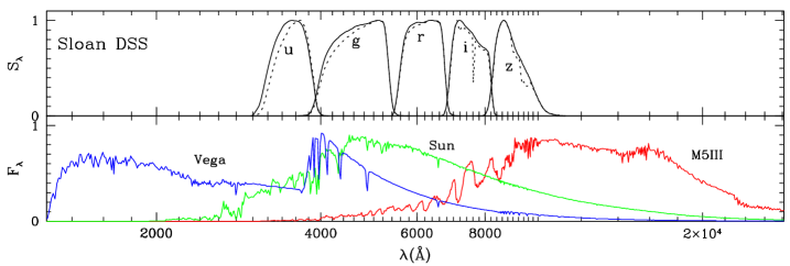
Figure 1: The SDSS filter+detector transmission curves $S_{\lambda}$ adopted in this work. They refer to the filter and detector throughputs as seen through airmasses of 1.3 (dashed lines) at Apache Point Observatory. For the sake of comparison, the curves for a null airmass (solid lines) are also presented. All curves are re-normalized to their maximum value of $S_{\lambda}$. The bottom panel presents the spectra of Vega (A0V), the Sun (G2V), and a M5 giant, in arbitrary scales of $F_{\lambda}$. The $\lambda$ scale here adopted is the same as in Figure 3 of Paper I.

The SDSS photometric system is defined by Fukugita et al. (1996); in this paper, it is described by means of normal AB magnitudes. Later on, Lupton et al. (1999) devised a modified way of expressing magnitudes – namely a change from a logarithmic to a inverse hyperbolic sine function of flux – that has been adopted by the SDSS project. It is worth discussing both cases separately.

2.1 Isochrones in the usual AB magnitude scale

As described by Fukugita et al. (1996), the SDSS uses an AB magnitude system (Oke & Gunn 1983), which considerably simplifies the derivation of bolometric correction tables: The zero-points are completely defined by using a synthetic spectrum of constant flux per unit frequency, without making any reference to the spectrum of real stars. This is detailed in Section 2.3.2 of Paper I. Here, suffice it to recall that the adopted reference spectra and magnitudes are $f_{{\rm AB},\nu}^{0}=3.631\times 10^{-20}\,\,\,{\rm erg\,s^{-1}\,cm^{-2}\,Hz^{-1}}$, and $m_{{\rm AB},\nu}^{0}=0$ for all filters, respectively.

Therefore, the bolometric corrections and AB magnitudes of the SDSS system have been computed in the same way used in Paper I to generate HST/WFPC2 and HST/NICMOS AB magnitudes.

For the transmission curves $S_{\lambda}$ of the $ugriz$ filters, we use the SDSS filter curves available from the DR1 webpages. They are illustrated in Fig. 1, and include the filter and detector throughputs, and the atmosphere as seen through an airmass of 1.3 at Apache Point Observatory. Details of these transmission curves may change as future measurements of the filters are done.

It is worth mentioning that Fukugita et al. (1996) use the spectra of real stars – namely the Oke & Gunn (1983) spectrophotometric standards – in order to define the zero-points of SDSS photometry, even suggesting a revision in the spectra of these spectrophotometric standards. But actually these revisions regard only the transformation of observations into the standard ABmag system, and do not imply any change in the definition of AB magnitudes. Therefore, the zero-points of our theoretical models are not affected: they are, by construction, strictly in the ABmag system.

2.2 Conversion to the Lupton et al. modified magnitude scale

Lupton et al. (1999) suggested a modified magnitude definition where the classical logarithmic scale

$$m(f)=m_{0}-2.5\log f$$ (2)

(where $m$ is a magnitude, $m_{0}$ is a zero-point, and $f$ is the photon flux as integrated over a filter pass-band) is replaced by an inverse hyperbolic sine function

$$\mu(f)=(m_{0}-2.5\log b^{\prime})-a\sinh^{-1}(f/2b^{\prime})\,\,\,$$ (3)

where $a=2.5\log e$, and $b^{\prime}$ is the constant (in photon flux units) that gives $\mu(0)=m_{0}-2.5\log b^{\prime}$ for a null flux. In practice, $b^{\prime}$ is related to the limiting magnitude of a given photometric survey, and has to be furnished together with the apparent $\mu$ in any of its data releases. This magnitude definition reproduces the traditional definition for objects measured with a signal-to-noise $>5$, avoids problems with negative fluxes for very faint objects, and retains a well-behaved error distribution for fluxes approaching zero. Hence it is primarily of importance for objects near the detection limit.

It is clear that this definition of magnitude is not compatible with the formalism we adopt to derive bolometric corrections. Actually, basic quantities like bolometric corrections, absolute magnitudes, and distance modulus, cannot be defined in any simple way if we use the Lupton et al. scale, because it is a non-logarithmic one. As a corollary, we can say that such a scale represents a convenient way to express apparent magnitudes and colours near the survey limit (as demonstrated by Lupton et al. 1999), but represents a complication if we want to represent absolute magnitudes.

Considering this, we do not even try to express our theoretical models by means of Lupton et al. (1999) modified magnitude scale. We do, however, provide a prescription of how to convert absolute magnitudes $M_{S_{\lambda}}$ – given by our models in the AB system – into an apparent $\mu_{S_{\lambda}}$ – as given in the SDSS data releases. This can be done in the following way:

1. convert from absolute to apparent magnitudes using the usual definitions of distance modulus and absorption, i.e., $m_{S_{\lambda}}=M_{S_{\lambda},0}+(m-M)_{0}+A_{S_{\lambda}}$;

2. convert from classical apparent magnitudes to a photon flux, i.e. $f=\int(\lambda/hc)\mbox{${\rm d}$}\lambda$ in the case of ABmags; this requires knowledge of the effective throughputs in each pass-band $S_{\lambda}$, referring to the complete instrumental configuration (pratical hints on this step, regarding SDSS DR1 data, can be found in the URL http://www.sdss.org/dr1/algorithms/fluxcal.html);

3. convert the photon flux to Lupton et al. (1999) modified magnitude scale by means of Eq. 3, using the $b^{\prime}$ constant typical of the observational campaign under consideration.

Of course, the procedure is not as simple as one would like. Since at good signal-to-noise ratios ($f>b^{\prime}$) the Lupton et al. scale coincides with the classical definition of magnitudes, the question arises whether it is necessary at all to convert models to Lupton et al. (1999) scale. In fact, for most analyses of stellar data it will not be worthwhile, since one is rarely tempted to derive astropysical quantities from stars measured with large photometric errors.

For diffuse and faint objects like distant galaxies, however, the situation might well be the opposite one: even relatively noisy data may contain precious astrophysical information. Useful hints about the dominant stellar populations may result, for instance, from a comparison between the integrated magnitudes and colours of single-burst stellar populations (provided in this paper in the usual magnitude scale) to those of faint galaxy structures from SDSS (given in the Lupton et al. scale). If this is the case, the conversion problem has to be faced.

2.3 Extinction coefficients

Table 1: Computed $A_{\lambda}/A_{V}$ values for a few stars and extinction cases.

Star:			extinction:		$A_{\lambda}/A_{V}$ for:
$T_{\rm eff}$	$\log g$	$[{\rm M/H}]$	$A_{V}$	$R_{V}$	$u$	$g$	$r$	$i$	$z$
5777	4.44	0	0.5	3.1	1.574	1.199	0.879	0.675	0.490
5777	4.44	0	1.0	3.1	1.574	1.196	0.878	0.674	0.490
5777	4.44	0	2.0	3.1	1.573	1.190	0.876	0.672	0.489
5777	4.44	0	3.0	3.1	1.571	1.184	0.875	0.671	0.488
5777	4.44	0	1.0	5.0	1.331	1.126	0.903	0.732	0.564
3500	0.00	0	0.5	3.1	1.551	1.154	0.874	0.662	0.481
3500	2.00	0	0.5	3.1	1.551	1.175	0.877	0.660	0.479
3500	4.50	0	0.5	3.1	1.558	1.178	0.874	0.663	0.482
3750	0.00	0	0.5	3.1	1.553	1.154	0.872	0.667	0.484
3750	2.00	0	0.5	3.1	1.553	1.170	0.874	0.665	0.484
3750	4.50	0	0.5	3.1	1.558	1.178	0.874	0.665	0.485
4000	0.00	0	0.5	3.1	1.558	1.156	0.872	0.670	0.485
4000	2.00	0	0.5	3.1	1.557	1.170	0.873	0.669	0.486
4000	4.50	0	0.5	3.1	1.560	1.180	0.874	0.668	0.486
4500	0.00	0	0.5	3.1	1.567	1.166	0.875	0.672	0.487
4500	2.00	0	0.5	3.1	1.569	1.175	0.875	0.672	0.487
4500	4.50	0	0.5	3.1	1.568	1.185	0.875	0.672	0.488
5000	0.00	0	0.5	3.1	1.564	1.179	0.876	0.673	0.489
5000	2.00	0	0.5	3.1	1.570	1.184	0.877	0.673	0.489
5000	4.50	0	0.5	3.1	1.574	1.189	0.877	0.673	0.489
6000	2.00	0	0.5	3.1	1.565	1.204	0.879	0.675	0.490
6000	4.50	0	0.5	3.1	1.574	1.202	0.879	0.675	0.490
8000	4.50	0	0.5	3.1	1.573	1.221	0.883	0.678	0.491
10000	4.50	0	0.5	3.1	1.573	1.231	0.885	0.679	0.491
12500	4.50	0	0.5	3.1	1.578	1.235	0.886	0.680	0.492
15000	4.50	0	0.5	3.1	1.581	1.237	0.886	0.680	0.493
20000	4.50	0	0.5	3.1	1.585	1.240	0.886	0.680	0.494
30000	4.50	0	0.5	3.1	1.588	1.243	0.887	0.681	0.495
40000	4.50	0	0.5	3.1	1.589	1.245	0.887	0.681	0.495
50000	5.00	0	0.5	3.1	1.590	1.246	0.887	0.681	0.495
4000	2.00	-2	0.5	3.1	1.560	1.173	0.873	0.670	0.487
4000	4.50	-2	0.5	3.1	1.564	1.179	0.872	0.670	0.487
6000	4.50	-2	0.5	3.1	1.576	1.209	0.879	0.675	0.490
10000	4.50	-2	0.5	3.1	1.573	1.231	0.885	0.679	0.491
Schlegel et al. (1998):					1.579	1.161	0.843	0.639	0.453
Fiorucci & Munari (2003), $R_{V}=3.1$:					$1.61^{1.58}_{1.69}$	$1.19^{1.16}_{1.20}$	$0.83^{0.84}_{0.85}$	$0.61^{0.61}_{0.64}$	$0.45^{0.45}_{0.48}$

$T_{\rm eff}$	$\log g$	$[{\rm M/H}]$	$A_{V}$	$R_{V}$	$U$	$B$	$V$	$R$	$I$	$J$	$H$	$K$
5777	4.44	0	0.5	3.1	1.562	1.298	1.006	0.826	0.600	0.292	0.186	0.116
Schlegel et al. (1998)
(for CTIO and UKIRT filters):					1.521	1.324	0.992	0.807	0.601	0.276	0.176	0.112
Fiorucci & Munari (2003), $R_{V}=3.1$:					$1.58^{1.54}_{1.62}$	$1.31^{1.25}_{1.32}$	$0.99^{1.00}_{1.00}$	$0.77^{0.75}_{0.79}$	$0.56^{0.56}_{0.58}$	$0.27^{0.27}_{0.28}$	$0.17^{0.17}_{0.18}$	$0.11^{0.11}_{0.12}$

The basic formalism of synthetic photometry as introduced in Paper I, allows an easy assessment of the effect of interstellar extinction on the output data. As can be readily seen in Eq. (2), each stellar spectrum $F_{\lambda}$ in our database can be reddened by applying a given extinction curve $A_{\lambda}$, and hence the bolometric corrections computed as usual. The difference between the BCs derived from reddened spectra and the original (unreddened) ones, divided by the amount of total reddening in a reference passband (say $A_{V})$, gives the so-called extinction coefficients

$$A_{\lambda}/A_{V}=\frac{BC_{S_{\lambda}}(A_{V})-BC_{S_{\lambda}}(0)}{A_{V}}$$ (4)

These quantities are of course useful for consistently computing the amount of extinction expected in different passbands.

In order to derive $A_{\lambda}/A_{V}$ values, we first assume the Cardelli et al. (1989) extinction curve for a typical Galactic total-to-selective ratio of $R_{V}=A_{V}/E_{B-V}=3.1$. The derived values of $A_{\lambda}/A_{V}$ are tabulated in Table 1, for a few different stellar spectra (from ATLAS9 models) ranging in $T_{\rm eff}$, $\log g$, and metallicity $[{\rm M/H}]$.

The first line in the table presents our reference $A_{\lambda}/A_{V}$ values, namely those derived for a Sun-like yellow dwarf ($\mbox{$T_{\rm eff}$}=5777$ K, $\log g=4.44$, $[{\rm M/H}]=0$; Kurucz 1993) with low reddening and a normal $R_{V}=3.1$ extinction curve. They will be adopted in the simple comparisons with data to follow in Sect. 3. For the same star and for the sake of comparison, $A_{\lambda}/A_{V}$ coefficients are presented also for the Johnson-Cousins-Glass system as defined by Bessell & Brett (1988) and Bessell (1990).

Then, the table presents a sequence of $A_{\lambda}/A_{V}$ ratios for increasing values of total extinction $A_{V}$ at constant $R_{V}=3.1$. It illustrates that $A_{\lambda}$ has a very small, non-linear trend with $A_{V}$ (see also Grebel & Roberts 1995). The $R_{V}=5.0$ value, suitable for dense star-forming regions as the Orion Nebulae, is also considered. In this case, $A_{\lambda}/A_{V}$ ratios become very different from the previous ones.

Most of Table 1 is dedicated to present $A_{\lambda}/A_{V}$ ratios obtained for stars of different $T_{\rm eff}$ and $\log g$, for both solar and metal poor compositions ($[{\rm M/H}]=0$ and $-2$, respectively), in the limit of low total extinction and for $R_{V}=3.1$. They are all derived from Bessell et al. (1997) ATLAS9 spectra. It can be noticed that $A_{\lambda}/A_{V}$ depends in a non-negligible way on $T_{\rm eff}$ and $\log g$, and to a much lower extent on $[{\rm M/H}]$. All these effects are thoroughly discussed in Grebel & Roberts (1995). For the present paper, suffice it to mention that we are able to provide $A_{\lambda}/A_{V}$ values for any other extinction curve and stellar spectra, upon request.

We also note that the extinction coefficients we find for the SDSS system are somewhat different from those mentioned in the SDSS Early Data Release by Stoughton et al. (2002), and derived by Schlegel et al. (1998; see values in Table 1). Assessing the detailed reasons for these differences is beyond the scope of this paper. Anyway, we remark that Schlegel et al. (1998) compute their extinction values using a very different spectrum (an elliptical galaxy one), which is likely one of the main sources of the discrepancy. On the other hand, our $A_{\lambda}/A_{V}$ values are also different from those computed by Fiorucci & Munari (2003) using essentially the same stellar spectra and extinction curves. In this latter case, the discrepancies are likely to be ascribed to the different numerical methods and, to a lower extent, to their use of Fukugita et al. (1996) filter transmission curves instead of DR1 ones. Among the possible differences in numerical methods, it is remarkable that both Schlegel et al. (1998) and Fiorucci & Munari (2003) use the concept of photon-energy integration in their definition of $A_{\lambda}$, instead of the photon-count integration we perform in ours Eq. 2 (see Paper I for a discussion on this topic).

2.4 Presently available isochrones

All isochrone sets from the Padova group have been converted into the SDSS ABmag system. Their input stellar tracks and particularities are listed in Table 1 of Paper I. Here, suffice it to recall the main isochrone sets available:

• A “basic set” derived by using the Girardi et al. (2000) evolutionary tracks for $0.15\leq M/\mbox{$M_{\odot}$}\leq 7$ together with previous Padova tracks for massive stars of $M\geq 7\mbox{$M_{\odot}$}$ (from Bressan et al. 1993; Fagotto et al. 1994ab; Girardi et al. 1996). This set has also been complemented with newest tracks (Girardi et al. 2003) for massive $Z=0.001$ stars, and covers a very wide range of metallicities (from $Z=0.0001$ to $0.03$). It also represents a sort of fusion between the Bertelli et al. (1994) isochrones for ages $t\la 10^{8}$ yr, with the Girardi et al. (2000) ones for $t>10^{8}$ yr;

• A set for metal-free ($Z=0$) stars, from Marigo et al. (2001).

• The Salasnich et al. (2000) isochrones for both solar-scaled and $\alpha$-enhanced chemical compositions, and moderate to high metallicity range (from $Z=0.008$ to $0.07$).

• The Marigo & Girardi (2001) isochrones, derived by complementing the Girardi et al. (2000) tracks with the very detailed TP-AGB sequences from Marigo et al. (1999), available for $Z=0.004$, $0.008$ and $0.019$.

In the following sections, we will only use the above-mentioned “basic set” of isochrones, which covers the widest range of ages and metallicities.

The list of isochrone sets is in continuous expansion and subject to revision at any time (see for instance the main addition anticipated by Marigo et al. 2003). Importantly, the present paper does not present any new isochrone set, but just their transformation into a new system. Users of SDSS isochrones should better refer also to the original source of stellar data, listed in the items above and detailed in the electronic database that contains all data tables.

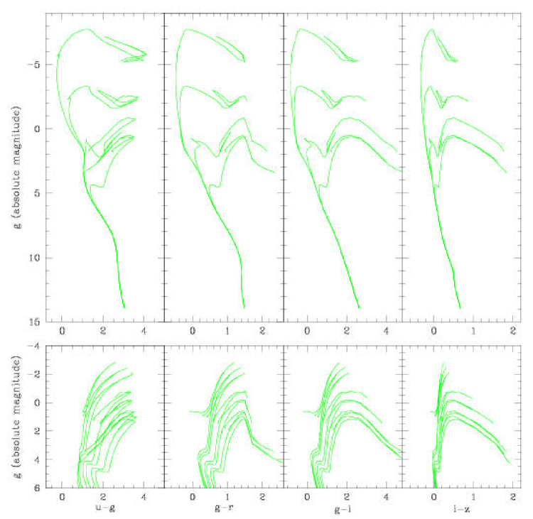
Figure 2: Isochrones in several CMDs of SDSS photometry. Top panels: a sequence of solar-metallicity ($Z=0.019$) isochrones of increasing ages, namely $10^{7}$, $10^{8}$, $10^{9}$, $10^{10}$ yr, going from the brightest to faintest turn-off. Bottom panels: a sequence of 12-Gyr old isochrones of increasing metallicities, namely $Z=0.0001$, $0.0004$, $0.001$, $0.004$, $0.008$, $0.019$ and $0.03$, going from the bluest to the reddest turn-off.

Figure 2 shows two different isochrone sequences – taken from the “basic set” – in CMDs of SDSS photometry: one of varying age at solar metallicity, and another of varying metallicity at old ages. The figure well illustrates the expected locus of some main evolutionary phases (main sequence, RGB, red clump, HB, cepheid loop, AGB, red supergiants), as well as the expected appearance of CMDs for star clusters, in this yet unfamiliar photometric system.

3 Tests using DR1 data

We chose three different objects in order to test the isochrones: Two globular clusters (Palomar 5 and NGC 2419) and one nearby dwarf spheroidal galaxy (Draco), which are all three included in the DR1 database. In fact, these three objects are the only globular clusters and nearby resolved dwarf galaxies currently available from the public SDSS database. All three objects have been extensively studied in the past in standard photometric systems such as Johnson-Cousins and also have spectroscopic metallicity measurements. We can use them now for isochrone consistency checks for old populations at intermediate ($-1.4$ dex) and low ($\sim-2$ dex) metallicities. We require that Johnson and SDSS data can be fit with isochrones in these two photometric systems that use the same parameters (internal consistency), and that these parameters are consistent with previous results from the literature (external consistency).

Before proceeding, we recall that a preliminary version of our isochrones – using 2001 filter tranmission curves from Strauss & Gunn, as retrieved from http://archive.stsci.edu/sdss/documents/response.dat – have been recently compared to data for the open cluster M 48 by Rider et al. (2004). Their data were obtained using $u^{\prime}g^{\prime}r^{\prime}i^{\prime}z^{\prime}$ filters available at the CTIO Curtis-Schmidt, US Naval Observatory (USNO) 1.0m, and SDSS 0.5m Photometric telescopes. Thus, Rider et al.’s work shall be considered as an additional test to the theoretical isochrones we are presenting in this paper.

3.1 Palomar 5

Palomar 5 is a sparse halo globular cluster at a distance of $\sim 23$ kpc (Harris 1996). Its current mass is only 4.5 to $6\cdot 10^{3}$ M_⊙ (Odenkirchen et al. 2002), and it is undergoing significant tidal disruption as evidenced by its two well-defined, symmetric tidal tails (Odenkirchen et al. 2001a, 2003; Rockosi et al. 2002). With a metallicity of $\mbox{\rm[{\rm Fe}/{\rm H}]}\sim-1.4$ dex (Harris 1996), it is the most metal-rich resolved single-age stellar population presently available from the public SDSS photometry database. Therefore we will use this cluster despite its sparseness for our isochrone comparison.

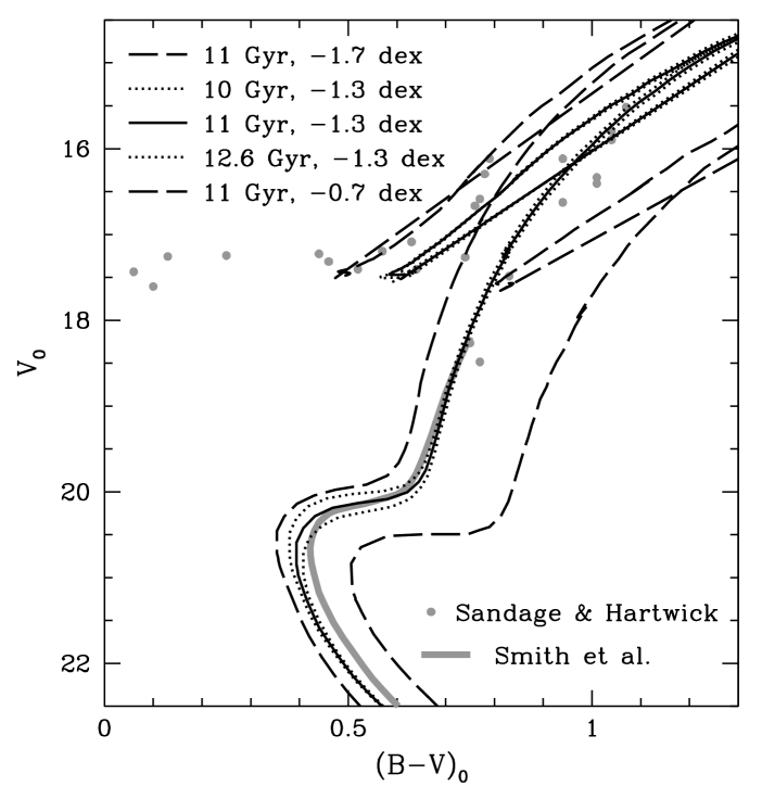
Figure 3: Reddening-corrected color-magnitude diagram of Palomar 5 in the Johnson $B$ and $V$ filters. The data points (grey dots) were taken from Sandage & Hartwick (1977). The thick grey solid line represents the mean location of the lower red giant branch, subgiant branch, and main sequence as given by Smith et al. (1986). The thinner black lines – dashed, dotted, and solid – are Johnson isochrones from Girardi et al. (2002) as detailed in the legend (sequence from left to right). The $Z=0.001$ ($-1.3$ dex) isochrone with an age of 11 Gyr provides the closest match to the Smith et al. fiducial. Older and younger isochrones (dotted lines) have main-sequence turn-offs that are too faint or too luminous, respectively.

We first attempt to constrain the age and other parameters of Pal 5 using Johnson photometry data that extend well below the main-sequence turn-off. If the Johnson and the SDSS isochrones are internally consistent, then the parameters that we derive from the Johnson data should also apply to the SDSS data. Published Johnson $B$, $V$ photometry is available from Sandage & Hartwick (1977) and Smith et al. (1986). In Fig. 3, we show data points from Sandage & Hartwick’s photoelectric study and the fiducial sequence derived by Smith et al., together with isochrones from Girardi et al. (2002) in the generic Johnson system. We find the $Z=0.001$ (or $\mbox{\rm[{\rm Fe}/{\rm H}]}\sim-1.3$ dex) and $\log(t)=10.05$ (11 Gyr) isochrone to provide the closest fit to the overall slope of the fiducial and to the location of the main-sequence turn-off. This metallicity is in good agreement with the literature value (see above). We also found that the use of a slightly higher reddening than found in earlier studies (cf. Sandage & Hartwick 1977), $\mbox{$E_{B\!-\!V}$}=0.04$ mag, improves the fit. The deviations between the fiducial main sequence and the isochrone along the color axis may be caused, in part, by differences between the filter and detector combination used by Smith et al. and the Johnson filter definition used by Girardi et al., and by the procedure used by Smith et al. (1986) to derive the mean fiducial values. For instance, Smith et al. do not find evidence for a binary main sequence and consequently do not correct for it, while new deep CCD data (Koch et al. 2003, in prep.) show clear evidence for the presence of binaries.

The SDSS photometric database provides an estimate of the Galactic foreground extinction along the line of sight of each catalogued object, which is based on the extinction maps of Schlegel, Finkbeiner, & Davis (1998) and which thus applies primarily to objects outside of the Milky Way. The mean reddening value resulting from the Schlegel et al. (1998) maps is $\langle\mbox{$E_{B\!-\!V}$}\rangle=0.056$ mag. We choose to adopt the same constant reddening value of $\mbox{$E_{B\!-\!V}$}=0.04$ mag as used above for the Johnson photometry and convert it into the SDSS system using the extinction coefficients given in Table 1. As an investigation into large-scale extinction properties in the region of Pal 5 has shown, the reddening at the location of the cluster is low and homogeneous (see Odenkirchen et al. 2003, Figure 12), which further supports our use of one single, fixed reddening value. The amount of interstellar extinction also depends on the target star’s effective temperature, surface gravity, and metallicity as detailed in Grebel & Roberts (1995), and as illustrated for SDSS filters in Table 1. In the limit of low extinction (for say $\mbox{$E_{B\!-\!V}$}\la 0.1$), the magnitude of these effects is small, so that we do not take them into account in this section.

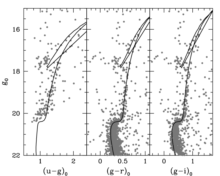
Figure 4: Color-magnitude diagrams of Palomar 5 in different SDSS filters. The grey dots represent stars with photometric uncertainties $<0.1$ mag. The solid line is one of our new SDSS isochrones with an age of $\log(t)=10.05$ and $Z=0.001$, i.e., with the best-fit parameters as found in Fig. 3. This isochrone provides the closest match to the SDSS data.

Fig. 4 shows the resulting, de-reddened CMDs of Pal 5 using different SDSS filter combinations. Only stars whose photometric uncertainties are below 0.1 mag are plotted. Colors including the SDSS $z$-band were omitted, since no well-defined giant branch was visible for Pal 5. Our SDSS isochrones were shifted by the appropriate distance modulus (see above). As before, an isochrone with a metallicity of $Z=0.001$ and an age of 11 Gyr ($\log t=10.05$) approximates the observed CMD best, especially in the part corresponding to the RGB. A careful inspection of the figure however reveals that below the turn-off level this isochrone runs slightly to the blue ($\la 0.1$ mag) with respect to the mean colour of main sequence stars. Such a discrepancy could be caused either by a real colour shift in the models, or by the presence of binaries in the data.

3.2 NGC 2419

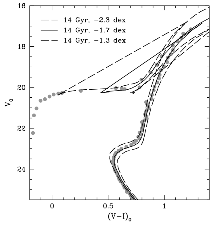
Figure 5: $V$, $I$ color-magnitude diagram of NGC 2419. The grey dots mark the fiducial derived for this cluster by Harris et al. (1997). Also shown are three of our new SDSS isochrones with an age of $\log(t)=10.10$. Of these, the $Z=0.0004$ isochrone ($\mbox{\rm[{\rm Fe}/{\rm H}]}=-1.7$ dex; solid line) provides the closest match to the data and best reproduces the slope of the red giant branch when using the reddening and distance modulus found by Harris et al. (1997).

NGC 2419 is a massive, very distant outer halo globular cluster. Harris et al. (1997) quote a distance of $\sim 81$ kpc and a metallicity of $\mbox{\rm[{\rm Fe}/{\rm H}]}=-2.14$ dex. The $V$, $I$ data of Harris et al. extend well below the main-sequence turn-off of NGC 2419 near $V\sim 24$ mag. Since the SDSS limiting magnitude is much brighter than this, we use the fiducial points provided by Harris et al. to find the best-fitting Padua isochrone. For a reddening of $\mbox{$E_{B\!-\!V}$}=0.11$ mag as suggested by Harris et al. (1997), we find the closest fit for an isochrone with $\log(t)=10.15$ ($\sim 14$ Gyr) and $Z=0.0004$ ($\mbox{\rm[{\rm Fe}/{\rm H}]}\sim-1.7$ dex). The $Z=0.0001$ isochrone (Fig. 5), while being closest to the spectroscopic metallicity, is too steep and does not reproduce the slope of the red giant branch. This appears to be a general property of metal-poor Padua isochrones (see, e.g., Fig. 5 in Grebel 1999) and does not affect the goals of our present work, since we care primarily about establishing an intrinsically consistent set of isochrones in different photometric systems.

Figure 6: Johnson/Kron-Cousins $BVRI$ color-magnitude diagrams of NGC 2419 based on Stetson’s (2000) homogeneous photometry (grey dots). Superimposed we show Johnson/Kron-Cousins isochrones from Girardi et al. (2000) with the same parameters as in Fig. 5. As before, the $-1.7$ dex, 14 Gyr isochrone matches the multi-color data well, apart from a general shift to redder colours and fainter magnitudes.

We note that Harris et al. (1997) found NGC 2419 to be essentially indistinguishable in age from the ancient, metal-poor halo globular cluster M92, provided that these two clusters do not show pronounced differences in their chemical abundance ratios, particularly in their $\alpha$ elements. In this context it is interesting to note that Newberg et al. (2003) recently found NGC 2419 to be probably associated with a distant tidal arm of the Sagittarius dwarf spheroidal galaxy (see also Zhao 1998). While this could be taken as an indication that this cluster’s $\alpha$ element abundances differ from those measured in the Galactic halo, Shetrone, Côté, and Sargent (2001) found the element ratios in NGC 2419 very similar to those in M92 (based on the analysis of one star). Hence we cautiously consider it justified to use isochrones with $\alpha$ element ratios akin to those in the Galactic halo.

The $Z=0.0004$, 14 Gyr isochrone with the above reddening and distance also provides a good fit to CMDs of NGC 2419 in other Johnson/Kron-Cousins bands as shown in Fig. 6. There seems to be a general shift of the isochrones to redder colours and fainter magnitudes, which might be indicating an overestimation of the reddening towards this cluster. Such a shift was not apparent in the former Fig. 5, hence suggesting an off-set in the photometric data rather than in the models. The input photometry in this case was taken from Stetson’s (2000) on-line database of homogeneous $BVRI$ photometry for star clusters and resolved galaxies, which includes only photometry based on multiple independent measurements.

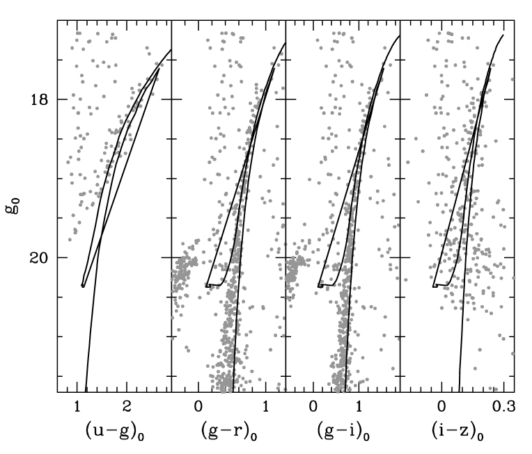
Figure 7: SDSS ugriz color-magnitude diagrams of NGC 2419 for stars with photometric uncertainties $<0.1$ mag (grey dots). Superimposed we show our new SDSS isochrone with the parameters found to work best for Johnson/Kron-Cousins photometry (see Fig. 5 and 6). This isochrone also provides a fully consistent fit to the multi-color SDSS data.

In Fig. 7 the SDSS $ugriz$ photometry is shown together with the newly transformed isochrone that also provided the best fit to the Johnson/Kron-Cousins data. As before for the Johnson/Kron-Cousins photometry, we used a fixed reddening of $\mbox{$E_{B\!-\!V}$}=0.11$ mag, which we transformed using the SDSS extinction coefficients listed in Table 1. As in the case of Johnson/Kron-Cousins photometry, there is a good match between the SDSS isochrone and the SDSS data but for a slight overall shift of the isochrones to redder colours and fainter magnitudes. The magnitude of this shift in the different passbands indicates that a better match to the NGC 2419 data could be obtained with smaller values of reddening, closer to $\mbox{$E_{B\!-\!V}$}=0$ than to the value of $\mbox{$E_{B\!-\!V}$}=0.11$ mag here considered. If we assume this is the case, the good overall fit of isochrones to NGC 2419 data shows that we get consistent results also for metal-poor abundances.

3.3 Draco

While the dwarf spheroidal galaxy Draco is dominated by old populations, it differs from single-age, single-population objects like globular clusters in showing a considerable abundance spread of more than one dex in [Fe/H] (Lehnert et al. 1992; Shetrone, Bolte, & Stetson 1998; Shetrone et al. 2001; and references therein). Draco’s mean spectroscopic metallicity is $\sim-1.9$ dex according to Lehnert et al. (1992; based on 14 red giants) and $\sim-2.0$ dex following Shetrone et al. (2001; based on six giants). Aparicio et al. (2001) found a mean photometric metallicity of $-1.8$ dex when applying Padua isochrones to Johnson $B,R$ photometry. Bellazzini et al. (2002) compared $V$, $I$ photometry of Draco’s red giants to globular cluster fiducials and derived a mean photometric metallicity of $-1.7$ dex. Aparicio et al. (2001) did not see indications of a metallicity gradient across the galaxy within the $\sim 1$ deg² area they studied. On the other hand, Klessen, Grebel, & Harbeck (2003), who analyzed a much larger area based on SDSS data, noted a population gradient in the sense that blue horizontal branch stars show a spatially more extended distribution than red horizontal branch stars. Spatial gradients in the horizontal branch morphology are commonly found in dwarf spheroidal galaxies (see Hurley-Keller, Mateo, & Grebel 1999; Grebel 2000; Harbeck et al. 2001; Grebel, Gallagher, & Harbeck 2003) and are likely either due to age spreads in the central regions of these galaxies, due to metallicity spreads, or a combination thereof.

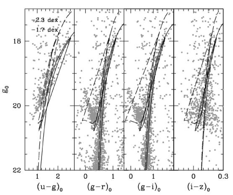
Figure 8: SDSS ugriz color-magnitude diagrams of the central $9^{\prime}\times 9^{\prime}$ of the Draco dwarf spheroidal galaxy for stars with photometric uncertainties $<0.1$ mag (grey dots). Superimposed we show our new SDSS isochrones for ages of $\log(t)=10.1$ and the parameters discussed in the text. The main concentration of the red giant branch of Draco lies blueward of the $-1.7$ dex isochrone (solid line).

In order to test the new SDSS isochrones, we confine ourselves to the central $9^{\prime}\times 9^{\prime}$ region of Draco, which has the added advantage of reducing the contribution of contaminating Galactic foreground stars. As described above, we are very likely sampling a mix of (predominantly old) populations with a range of metallicities and an age spread. The analysis by Aparicio et al. (2001), using Padua isochrones, does indeed suggest a range of ages. We therefore choose an age of $\log(t)=10.1$ for the SDSS isochrones, which corresponds roughly to the mean age indicated by the star formation histories of Aparicio et al. (2001). We adopt the Draco distance obtained through various methods by Bellazzini et al. (2002), i.e., $\sim 93$ kpc. The interstellar extinction along the line of sight to Draco is low but variable (see the extinction map in Odenkirchen et al. 2001b, their Fig. 1). We used both the individual, star-by-star Schlegel et al. (1998) extinction values available from the DR1 database and a constant value of $\mbox{$E_{B\!-\!V}$}=0.03$ mag together with the extinction coefficients in Table 1 and did not find qualitative differences in the resulting CMDs for the central region considered here.

The resulting SDSS CMDs are shown in Figure 8, using the above parameters and individual dereddening. The $Z=0.0004$ (or $\mbox{\rm[{\rm Fe}/{\rm H}]}=-1.7$ dex is closest to the main body of the red giant branch of Draco in the different filters and provides a red envelope. If we were to derive a mean metallicity from the comparison with the SDSS isochrones, it would be closer to the lower metallicity estimates ($-1.8$ to $-1.9$ dex). As pointed out by Shetrone et al. (2001), Draco’s [$\alpha$/Fe] ratio is lower by $\sim 0.2$ dex than what is found in the Galactic halo, which will affect age estimates when isochrones with Galactic halo $\alpha$ ratios are used, but this should not affect the internal consistency check for the SDSS isochrones presented here. Considering the photometric uncertainties and the known metallicity spread in Draco, we consider the comparison between the isochrones at fixed metallicity spacing with the multi-color SDSS data to demonstrate very satisfactory consistency.

4 Concluding remarks

We have computed bolometric corrections and extinction coefficients specific for the SDSS ABmag photometric system. They have been applied to transform previous Padova isochrones and integrated magnitudes of single-burst stellar populations into SDSS $ugriz$ absolute magnitudes. All data tables mentioned in this paper are available in the web site http://pleiadi.pd.astro.it. They have a structure similar to those already released with Paper I, and extended descriptions are also included in the form of electronic files.

Comparisons between the present isochrone sets and SDSS DR1 data, together with the recent results by Rider et al. (2004), are encouraging. Our hope is that this database will be useful for the analysis of the huge amount of photometric data that has been, and will yet be, released by the SDSS project. Obvious applications go from the derivation of parameters for star clusters and nearby dwarf galaxies (distances, reddenings, ages and metallicities), to the isolation of particular objects in colour-colour diagrams, to the application in analyses of star counts and Galactic structure. The further use of SDSS filters in other observatories, in programs not related to the original survey, may well expand the possible range of use for these tables.