XMM-Newton Observation of Solar Wind Charge Exchange Emission

Abstract

We present an XMM-Newton spectrum of diffuse X-ray emission from within the solar system. The spectrum is dominated by probable C VI lines at 0.37 keV and 0.46 keV, an O VII line at 0.56 keV, O VIII lines at 0.65 keV and $\sim 0.8$ keV, Ne IX lines at $\sim 0.92$ keV, and Mg XI lines at $\sim 1.35$ keV. This spectrum is consistent with that expected from charge exchange emission between the highly ionized solar wind and either interstellar neutrals in the heliosphere or material from Earth’s exosphere. The emission is clearly seen as a low-energy ($E<1.5$ keV) spectral enhancement in one of a series of four observations of the Hubble Deep Field North. The X-ray enhancement is concurrent with an enhancement in the solar wind measured by ACE, Wind, and SoHO spacecraft. The solar wind enhancement reaches a flux level an order of magnitude more intense than typical fluxes at 1 AU, and has a significantly enhanced O⁺⁷/O⁺⁶ ratio. Besides being of interest in its own right for studies of the solar system, this emission can have significant consequences for observations of cosmological objects. It can provide emission lines at zero redshift which are of particular interest in studies of diffuse thermal emission (e.g., O VII and O VIII), and which can therefore act as contamination in the spectra of objects which cover the entire detector field of view. We propose the use of solar wind monitoring data as a diagnostic to screen for such possibilities.

1 Introduction

Diffuse X-ray emission from the solar system was clearly observed during the ROSAT All-Sky Survey (RASS) as a background component with temporal variations on scales from a large fraction of a day to many days. These variations were dubbed Long-Term Enhancements (LTEs, Snowden et al. (1995)), and provided a significant background particularly at $1\over 4$ keV. Although the origin of these LTEs at the time was unknown, the LTEs were associated with solar wind parameters (Freyberg, 1994). With the observation of X-rays from comets (Lisse et al., 1996), emission from solar wind charge exchange (SWCX) between solar wind ions and neutral material within the heliosphere was demonstrated (Cravens, 1997). SWCX emission subsequently was suggested as the origin for LTEs (Cox, 1998; Cravens, 2000), and has recently been suggested as being responsible in quiescence for a significant fraction of diffuse X-ray emission at $1\over 4$ keV (Lallement, 2004; Robertson & Cravens, 2003b) previously attributed to the Local Hot Bubble (Snowden et al., 1998).

More recently, evidence for geocoronal emission (SWCX with exospheric material) has been detected in Chandra observations of the dark moon (Wargelin et al., 2004). This emission clearly originates in the near-Earth environment, which is consistent with the likely production of X-rays from the terrestrial magnetosheath (Robertson & Cravens, 2003a). The statistics of the dark moon data are somewhat limited but they clearly show excess O VII and O VIII emission.

Analysis of cometary X-ray spectra suggest that solar wind charge state composition and speed affect the X-ray emission (Lisse et al., 2001; Kharchenko et al., 2003; Schwadron & Cravens, 2000). Thus through a combination of techniques, including X-ray and neutral atom imaging among others, it may be possible to continuously monitor the solar wind from well inside Earth’s magnetosphere. However, the nature of solar system X-ray emission is strongly dependent on the point of view of the observer. While the observation of SWCX X-ray emission samples aspects of the solar system of interest to astronomers, the emission can also provide a contaminating component which strongly impacts observations of extended cosmic X-ray sources. The SWCX emission spectrum is dominated by highly ionized carbon, oxygen, neon, possibly iron, and magnesium lines, which are also of great astrophysical interest. (The oxygen lines are particularly important as they are commonly used for temperature and density diagnostics of thermal emission from diffuse plasmas.) For objects at zero redshift (i.e., emission from the Milky Way and nearby galaxies) where the emission is expected to fill the entire field of view of the detector, SWCX emission is indistinguishable from that of the object, except to the extent that temporal variation can be detected.

While there is likely to be SWCX emission at some quiescent level (Robertson & Cravens, 2003b; Lallement, 2004), the strongest emission will be associated with flux enhancements of the solar wind. These enhancements are long enough in duration that they can “contaminate” an entire observation, but variable enough that if there are multiple observations of a single target they can be identified, at least to some level. This was the basis of the LTE “cleaning” of the RASS (Snowden et al., 1995, 1997), and of ROSAT pointed observations which were typically distributed over the period of a few days if not weeks (Snowden et al., 1994).

In this paper we report the detection of SWCX emission during an XMM-Newton observation of the Hubble Deep Field North. We correlate that detection with a concurrent enhancement in the solar wind density observed by Advanced Composition Explorer (ACE), Solar and Heliospheric Observatory (SoHO), and Wind. In § 2 we present the data, data reduction, and analysis, in § 3 we discuss the results, and in § 4 we detail our conclusions both in regards to the emission itself and the implications for X-ray observations of more distant objects.

2 Data and Data Analysis

2.1 X-ray Data

2.1.1 Data Preparation

The SWCX emission discussed in this paper was observed in the fourth (2001 June 1–2) XMM-Newton pointing of the Hubble Deep Field North (HDF-N, $\alpha=12^{hr}36^{m}50.00^{s},\delta=+62^{\circ}13^{\prime}00.0^{\prime\prime}$, a project Guaranteed Time observation). Because of satellite constraints and the total length of the observation, it was broken into four segments (pointings), which were scheduled over a period of 16 days (Table 1 gives the specifics of the pointings). Because of this multiple coverage, the length of the individual pointings, and relative freedom from other non-cosmic backgrounds (most critically the soft proton flaring), the HDF-N observation was chosen as a test case for a new non-cosmic background modeling and subtraction method for XMM-Newton EPIC data (Kuntz et al., 2004). The serendipitous detection of the SWCX emission came from that testing.

Outside of time intervals obviously affected by proton flaring (which were removed for this analysis), the light curves for the observations were reasonably flat indicating at least a low if not zero level of residual flaring. Figure 1 shows the X-ray light curves for the non-flaring periods of the fourth observation, and also includes the ACE data (discussed below). The light curve for the 2–8 keV band is relatively constant but the 0.52–0.75 keV band (covering the O VII and most of the O VIII lines) shows a significant drop in the last quarter of the interval. We used this light curve to separate the spectrum into high and low states at $T=81578$ s in Figure 1 (22:39:38 UT on 2001 June 1; $T_{XMM}=107822378$ seconds after 0 UT, 1998 January 1, in the XMM-Newton time reference system). Table 1 also lists the average count rates in the 0.52–0.75 keV and 2–8 keV bands for the different pointings. The 2–8 keV band count rate is reasonably consistent among all of the pointings, as is the average count rate for the 0.52–0.75 keV band, except for the time period affected by the SWCX emission. The minor, but greater-than-statistical scatter of the X-ray count rates in Table 1 during the non-SWCX periods is likely due to the contribution of the unsubtracted particle background which is temporally variable, and/or variations in the residual SWCX emission.

Data from the full field of view were used in this analysis. They were conservatively filtered by screening the events using the parameters “FLAG==0” and “PATTERN$<$=12” (only the best events selected by position and limiting the CCD pixel pattern to legitimate quadruple and lower pixel-number events). The non-cosmic background was modeled using the method of Kuntz et al. (2004), which is currently limited to the EPIC MOS data (i.e., excludes data from the EPIC PN detector). The nominal non-cosmic background, which is dominated by the quiescent high-energy particle-induced background, is modeled using closed filter data scaled by data from the unexposed corners of the detectors in the individual observation. The scaling is energy dependent and based on the hardness and intensity of the corner data (which are temporally variable). This background modeling removes most of the non-cosmic background but unfortunately leaves untouched any backgrounds (particle or X-ray) originating in, or passing down the telescope tube (i.e., backgrounds which are blocked by the detector mask used in the closed-filter data collection). Most notably there are strong fluorescent Al K$\alpha$ and Si K$\alpha$ lines, and the possibility of soft protons at some quiescent level.

After background subtraction, the spectra from the full field of view of the first three HDF-N pointings and the low state of the fourth were reasonably statistically consistent, while the high-state data from the fourth pointing showed a strong enhancement at energies less than 1.4 keV (consistent with the light curve), which was dominated by line emission. The spectra at higher energies of all four pointings (including both high and low states of the fourth) were consistent with each other as expected from their average count rates (Table 1).

2.1.2 Spectral Fitting

For the spectral fits of the XMM-Newton X-ray data we used spectral redistribution matrices (RMFs) and effective areas (ARFs) produced by the project Standard Analysis Software (SAS) package (Version 5.4.1). Xspec (Version 11.2, Arnaud (2001)) was used to fit a model of the cosmic X-ray background (CXB), SWCX line emission (a number of discrete lines), probable residual soft proton contamination (represented by a power law not folded through the instrumental efficiency), and the two instrumental lines (Al K$\alpha$ and Si K$\alpha$) to the data after subtraction of the modeled non-cosmic background. In order to constrain the cosmic contribution to the spectrum, we simultaneously fit RASS data provided through the HEASARC X-Ray Background Tool, which uses data from Snowden et al. (1997) to create Xspec compatible spectra for selected directions on the sky. The spatial distribution of the CXB emission within the observed field, which includes the HDF-N, is relatively simple (by design there are no significantly bright point sources or extended objects in the field), and can be modeled using the four standard components listed in Kuntz & Snowden (2000): a cooler unabsorbed thermal component with $T\sim 0.1$ keV representing emission from the Local Hot Bubble (e.g., Snowden et al. (1998)), an absorbed cooler thermal component also with $T\sim 0.1$ keV representing emission from the lower halo, an absorbed hotter thermal component with $T\sim 0.6$ keV representing Milky Way halo or local group emission (e.g., McCammon et al. (2002)), and an absorbed power law with a spectral index of 1.46 representing the unresolved emission of AGN and other cosmological objects (e.g., Chen, Fabian, & Gendreau (1997)). The absorption was fixed to the Galactic column density of H I ($1.5\times 10^{20}$ cm^-2).

The spectral fitting was done simultaneously for eleven spectra: MOS1 and MOS2 data from the four observations with two spectra (high and low states) for the fourth observation, plus the RASS spectrum. The CXB model was fit to all spectra with no scaling between the different instruments besides the normalization for solid angle, which was fixed. The instrumental lines and soft-proton power law were fit only to the MOS data. The normalizations were allowed to differ between the MOS1 and MOS2 detectors but were constrained to be the same for all observations. The lines representing the SWCX were fit only to the MOS data from the high state of the fourth observation with the fit parameters constrained to be the same for the MOS1 and MOS2 data.

Figure 2 shows the results with the excess emission attributed to SWCX being clearly visible. The aluminum and silicon instrumental lines are the strong peaks at 1.49 keV and 1.74 keV, respectively. The SWCX emission was modeled by a set of Gaussians whose widths were set to zero except for the component at $E\sim 0.8$ keV which covers multiple lines from O VIII and possible lines from Fe XVII. The fitted line strengths are listed in Table 2. Two Gaussian lines with energies less than 0.5 keV were included in the fits, which can be associated with emission from highly ionized carbon (C VI at 0.37 keV and 0.46 keV). They are included in Table 2 with the following caveats. At energies less than 0.5 keV the energy resolution and effective areas of the MOS instruments fall off significantly and while the additional lines are necessary for reasonable fits ($\Delta\chi^{2}=39$ when one line is removed, $\Delta\chi^{2}=124$ when both lines are removed) the specific energies of the lines are not well constrained. However, there is no degrading of the quality of the fit when the line energies are fixed at the C VI values, and once the energies are fixed fluxes can be measured at better than the 3$\sigma$ level. Still, lines at other energies may fit the data as well so the attribution of the emission to C VI is not certain, it is however reasonable (cf. Kharchenko & Dalgarno (2000)). Note, however, that the addition of the C V line at 0.30 keV (also listed in Kharchenko & Dalgarno (2000)) did not improve the quality of the fit.

The power-law background component, which is assumed to represent residual soft proton contamination, was added to bring consistency between the RASS and MOS data. Because this power law is best fit without being folded through the MOS effective area, it is not due to X-rays originating externally to the satellite as they would be cut off at lower energies by the filter. The effective flux in this component is $\sim 0.85\times 10^{-8}$ ergs cm^-2 sr^-1 s^-1 while the flux of the cosmic background model is $7.15\times 10^{-8}$ ergs cm^-2 sr^-1 s^-1 in the 0.2–5.0 keV band, with $3.82\times 10^{-8}$ ergs cm^-2 sr^-1 s^-1 from the extragalactic power law. Figure 3 shows the MOS1 spectra from the first pointing and the high state of the fourth pointing along with the various components to the fit folded through the instrumental response.

The fit to the data is rather good with $\chi^{2}_{\nu}=1.13$ with 1922 degrees of freedom. The fitted values for the energies of the lines were consistent with the expected values in initial fits, and were subsequently fixed (except for the O VIII and the possible Fe complex at $E\sim 0.8$ keV). In general it is possible to move power between one spectral component and another in fits of such complex models as used here. The fitted parameters of the cosmic background model are, for example, strongly correlated. However, the measurement of the SWCX emission is very robust (as indicated by the quoted 90% probability statistical errors in the line fluxes listed in Table 2) as the background is so well constrained and the SWCX emission is in a limited number of discrete lines.

2.2 The Solar Wind

2.2.1 Monitoring the Solar Wind

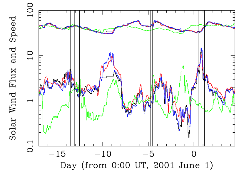
Figure 4: Measurement of the solar wind proton speed (upper curves, divided by 10 for clarity) and flux (lower curves) by four spacecraft during the period of the XMM-Newton HDF-N observations. The colors show data from ACE (black), Wind (red), SoHO (blue), and Ulysses (green). The deviation of the ACE from those of Wind and SoHO near day -9 is due to missing data. The vertical bars indicate the time intervals of the four XMM-Newton observations.

Solar wind speed and flux data from four spacecraft during the period of the HDF-N observations are shown in Figure 4. Three of them, ACE, Wind, and SoHO sample the near-Earth environment. ACE and SoHO have been, for the most part, located in halo orbits around the Sun-Earth libration point (L1, $\sim 1.5\times 10^{6}$ km, 235 $R_{E}$ from Earth). Wind has led a more peripatetic life and at the time of these measurements was no longer in an orbit around L1. ACE was launched on 1997 August 25, SoHO was launched on 1995 December 2, and Wind was launched 1994 November 1. The three spacecraft function, in part, as upstream monitors of the solar wind, the hot ($\sim 10^{6}$ K) plasma continually flowing from the Sun, and provide almost continual measurements of the solar wind density, speed, and magnetic field, among many other parameters. The fourth spacecraft, Ulysses, follows a high-inclination ($i\sim 79^{\circ}$), elliptical ($e\sim 0.6$ with a semi-major axis of $\sim 3.4$ AU) orbit around the Sun. Ulysses was launched 1990 October 6 and reached its roughly polar orbit after a fly-by of Jupiter.

At the time of these measurements, Earth was at $\sim 1.01$ AU, $0.0^{\circ}$ ecliptic latitude, and $\sim 251^{\circ}$ ecliptic longitude. The solar wind speed and flux data from the three near-Earth spacecraft are in reasonably good agreement showing the same structure (Figure 4). The major enhancements in the flux at all three spacecraft are roughly contemporaneous while discrepancies in the fluxes, although typically small but sometimes as much as a factor of two, may be in part due to the sometimes large separation ($>200~{}R_{E}$) between the spacecraft perpendicular to the Sun-Earth line. (Note that the deviation of ACE near day –9 in Figure 4 is due to missing data.) On the other hand Ulysses, which is in a polar orbit around the Sun, at this time was $\sim 1.34$ AU from the Sun with an ecliptic latitude of $\sim 5.6^{\circ}$ and an ecliptic longitude of about $\sim 339^{\circ}$. This location is farther from the Sun than the other spacecraft and $\sim 90^{\circ}$ ahead of the Earth. Thus, the Ulysses flux in Figure 4 is only qualitatively similar to that observed near Earth and shifted in time. These differences reflect the large scale structure of the interplanetary medium at this time. In addition, the Ulysses direction was $\sim 110^{\circ}$ away from the HDF-N, and so is not particularly relevant for the SWCX observation, but the comparison of the data provides an illustration of the variation of the solar wind from a uniform shell-like expansion.

2.2.2 The Solar Wind Enhancement

Although there exists considerable variability, solar wind speeds are typically about 450 km s^-1 (about 1 keV/nucleon) with fluxes at 1 AU of about $3\times 10^{8}$ cm^-2 s^-1 (Rucinski et al., 1996). The solar wind by is about 95% protons and 4% helium nuclei by number. High charge state heavy ions (i.e., other than protons and He⁺²) comprise less than 1% of the solar wind by number. These ions include carbon, dominated by charge states C⁺⁵ and C⁺⁶, oxygen, dominated by charge states O⁺⁶ and O⁺⁷, neon dominated by charge state Ne⁺⁸, and iron with a wide range of charge states sometimes as high as Fe⁺¹⁷ (Gloeckler et al., 1999; Collier et al., 1996). The solar wind source ion for the C VI lines in the X-ray spectrum is C⁺⁶ and the source ions for the O VII and O VIII lines are O⁺⁷ and O⁺⁸, respectively. Although typically the dominant charge states of solar wind oxygen are +6 and +7, under certain conditions, e.g., in the CME-related solar wind (coronal mass ejection), O⁺⁸ can be comparable to and even dominate the O⁺⁷ (Galvin, 1997). Ne⁺⁹ and Mg⁺¹¹, the solar wind source ions for Ne IX and Mg XI SWCX emission, have also been observed in the solar wind (A. B. Galvin, private communication). O VIII and Ne IX lines have been observed in cometary spectra (Kharchenko et al., 2003)

During the period of the 2001 June 1-2 XMM-Newton HDF-N pointing, the ACE Level 2 data show that the O⁺⁷/O⁺⁶ ratio was highly variable (Figure 1) compared to the first three pointings. The average ratio was enhanced by over a factor of two during the period when the SWCX emission was detected, and dropped by nearly an order of magnitude at the end of the pointing concurrent with the reduction in solar wind flux (Table 3). This large increase in the relative abundance of the higher ionization state during the SWCX period might suggest that the relative abundances of the ionization states of O⁺⁸, Ne⁺⁹, and Mg⁺¹¹ may also be significantly enhanced. Thus observation of SWCX emission from these species would be reasonable. However, preliminary results from ACE indicate that the O⁺⁸/O⁺⁷ ratio was actually relatively low at $\sim 0.05$ during the period of SWCX emission (Zurbuchen & Raines, private communication; the analysis continues). The picture becomes even more murky as the preliminary results also show the O⁺⁸/O⁺⁷ ratio increasing by a factor of 20 to 30 just as the SWCX emission and solar wind flux enhancement were cutting off. In addition, the (0.72–0.61 keV)/(0.52–0.61 keV) count rate ratio, which is a measure of the relative emission of O VIII and O VII, was consistent with a constant value ($\chi^{2}=25.8$ for 22 degrees of freedom) over the period of the SWCX emission. This is in spite of the variation in solar wind ionization state distributions.

The temporal variation of the X-ray data requires that the enhancement originates locally, at least in the solar system if not in the satellite/near-Earth environment. The presence of X-ray emission lines corresponding to the highly ionized charge states of oxygen, neon, and magnesium eliminates an origin internal to the satellite, and strongly implicates SWCX as the source of the emission enhancement. Furthermore, data from the Low Energy Neutral Atom LENA imager on the IMAGE spacecraft inside the magnetosphere during this event show an enhancement which suggests a neutral solar wind resulting from SWCX (Collier et al., 2001).

3 Discussion

3.1 Observation Geometry

The geometry of the 2001 June 1–2 observation with respect to the near-Earth environment is shown in Figure 5. The satellite is on the Sun side of the Earth with an angle of $\sim 83^{\circ}$ between the Sun and look directions. (Due to satellite constraints, the look direction of XMM-Newton must lie within $20^{\circ}$ of perpendicular to the Earth-Sun line.) The satellite and the observation line of sight are outside of Earth’s magnetosphere, based on the magnetospheric model of Petrinec & Russell (1996) (using a ram pressure of 7.4 nPa and a northward $B_{z}$). However, the line of sight may possibly pass through the magnetosheath relatively near the sub-solar point. Such an observation trajectory would sample the region of strongest production of X-rays by SWCX with exospheric material (Robertson & Cravens, 2003a). On the other hand, the trajectory may be entirely outside of the magnetosheath and therefore miss much of that emission. Because of this uncertain geometry, the SWCX emission can be from either exospheric material in Earth’s magnetosheath or from interstellar neutrals in the heliosphere, or more likely both (at least to some level). The detailed analysis of this geometry will be the subject of a following paper.

On a more global scale (with perhaps no particular relevance to this observation), during the time period of the 2001 June 1–2 observation the location of Earth in its orbit placed it almost directly upstream from the Sun relative to the flow of interstellar material through the solar system. (Earth is in the nominal upstream direction about 4 June.)

3.2 The SWCX Emission Spectrum

From Table 2 and Figure 2 it is clear that the excess emission can be well characterized by a limited number of highly significant lines with energies consistent with those expected from SWCX. With certain assumptions it is possible to use the observed X-ray line ratios to derive the concurrent ion ratios.

The fitted O VIII(0.65&0.81 keV)/O VII(0.56 keV) line ratio from Table 2 is 1.09. However, from Kharchenko et al. (2003), the $3^{3}P\rightarrow 1^{1}S$ and (at the 2% level) O VII $3^{1}P\rightarrow 1^{1}S$ lines contaminate the O VIII line at $\sim 0.65$ keV, and contribute $\sim 0.58$ cm^-2 sr^-1 s^-1 (using a factor of 0.079, derived from the relative intensities of the relevant lines in their Table 1, to scale from the O VII 0.56 keV flux). Correcting for this contribution, and assuming that the 0.81 keV emission is all from O VIII (see below), the O VIII(0.65&0.81 keV)/O VII(0.56&0.67 keV) emission ratio is then $\sim 0.94$ (Table 4). To convert the emission ratio to an ion number ratio we use the SWCX cross sections in Wargelin et al. (2004). The ratios between the hydrogen and helium SWCX cross sections for O⁺⁷ and O⁺⁸ are roughly the same, so we use the O⁺⁸/O⁺⁷ hydrogen cross section ratio of 1.66 to scale the flux ratio (this assumes that the scattering is optically thin and hydrogen is the dominant SWCX target neutral). This implies a solar wind O⁺⁸/O⁺⁷ abundance ratio of $0.57\pm 0.07$, which is somewhat higher than the more typical value of 0.35 (e.g., Schwadron & Cravens (2000)), but not unreasonable, as would be expected considering the enhancement of the O⁺⁷/O⁺⁶ ratio. However, as noted above, the preliminary O⁺⁸/O⁺⁷ ratio from ACE for the SWCX period is $\sim 0.05$, a significant discrepancy which we will revisit in a subsequent paper when the O⁺⁸/O⁺⁷ ratio data are more robust.

The energy and non-zero width for the fitted line at $E\sim 0.8$ keV is consistent with the expected O VIII Ly$\beta$ through Ly$\epsilon$ emission (Wargelin et al. (2004)). However, this is also the energy of possible Fe XVII emission. The ratio of the line strengths, Ly$\alpha$/Ly($\beta-\epsilon$), predicted by Wargelin et al. (2004) is 2.75 (with a $\sim 30\%$ uncertianty), while our measured ratio is $3.9\pm 0.8$. The two values are therefore in reasonably good agreement but the result does not rule out a contribution from Fe XVII. It does suggest that any Fe contribution to the observed flux is relatively limited.

3.3 Contemplation of the Temporal Variation

As measured by ACE, the solar wind during the 2001 June 1–2 period was in its “slow” state but with with fairly uncharacteristic ion abundances and flux during the enhancement period. At solar maximum, the solar wind at 1 AU shows a complex structure most likely resulting from the appearance of equatorial coronal holes. In contrast, at solar minimum, there tends to be a two state speed structure observed in the solar wind with fewer but well-formed transients such as coronal mass ejections and corotating interaction regions. Smith et al. (2003) provide a recent review of the complex variation of the solar wind during the solar cycle.

Solar wind fluxes during the first three XMM-Newton HDF-N observations were close to nominal levels (see Figure 4). However, during the observation on 2001 June 1-2, the solar wind flux observed by the ACE spacecraft was enhanced (as shown in Figures 1 and 4) by a factor of five over its typical value of $\sim 3\times 10^{8}$ cm^-2 s^-1. The average O⁺⁷/O⁺⁶ ionization state ratios for the observation (Table 3) were also significantly enhanced. This flux enhancement was relatively localized; it lasted 5-6 hours at a solar wind speed of $\sim 350$ km s^-1 implying a width of about 0.05 AU in the direction toward the Sun. The X-ray flux decrease at $T\sim 81000$ (2001 June 1, 22:30 UT) and the sharp drop in both the solar wind flux and O⁺⁷/O⁺⁶ ratio propagated to Earth from the L1 point (a delay of $\sim 4000$ s) are approximately contemporaneous, which suggests the X-ray flux is responding primarily to local solar wind conditions.

However, comparison of the solar wind flux and ionization state variation and X-ray light curves raises two critical questions. First, if the SWCX emission enhancement observed by XMM-Newton is due to a local phenomena, why is the large variation in solar wind flux not reflected in the X-ray intensity, or in a variation of the relative intensity of the O VII and O VIII emission? Over the course of 20 ks (roughly six hours) the solar wind flux increases by a factor of six while the X-ray light curve is essentially constant (Figure 1). If the SWCX emission was due solely to interactions with material from Earth’s exosphere, then the X-ray light curve should be closely linked to the solar wind flux measured by ACE at the L1 point. Robertson & Cravens (2003a) point out that the geometry of the magnetosheath is strongly affected by the density and velocity of the solar wind. With the observation geometry considered by Robertson & Cravens (2003a), i.e., looking out through the flanks of the magnetosheath, there is some buffering of the X-ray emission which smooths out the effects of strong solar wind enhancements. However, with the geometry of this observation where the line of sight possibly runs tangentially through their region of maximum X-ray emission near the magnetosheath sub-solar point, the situation is much more confused, and perhaps more likely to produce variations rather than to smooth out the SWCX flux.

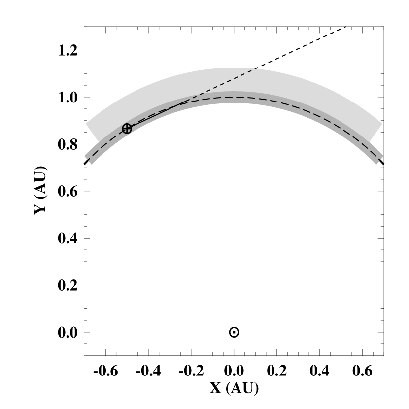
Figure 6: A cartoon of the solar system geometry for the observation of charge exchange from the density enhancement in the solar wind. The X,Y plane is defined by the Earth-Sun line and the look direction. The strongest part of the enhancement, shown as the darkest shading, lasts about a quarter of a day, which with the typical velocity of the solar wind (about a quarter of an AU per day) extends about 5% of an AU. The solar wind density was enhanced by about a factor of three (shown by the lighter shading) for more than a half a day preceding the main enhancement. The solid line from the Earth shows the look direction, and shows how the solar wind enhancement is sampled with the assumption of a spherically symmetric propagation.

Given the possible difficulty in turning the large variation of the solar wind flux into a relatively constant X-ray light curve, a possible solution might be to distribute the emission along the line of sight through the heliosphere. This would smooth out temporal variations originating with the solar wind. However, this brings up the second question. If the emission is distributed through the heliosphere why do the solar wind and X-ray enhancements cut off at nearly the same time? Note again the large differential variation in the solar wind flux as measured by ACE and Ulysses, up to a factor of 20, during SWCX observation. Figure 6 illustrates the observation geometry on a larger scale. Since the pointing direction is $\sim 83^{\circ}$ from the Earth-Sun line, the observation samples a relatively long path length through the solar wind enhancement with a heliocentric distance similar to that of the Earth. If the solar wind enhancement is a spherically symmetric shell moving outward there should still be a strong enhancement in the SWCX emission roughly concurrent with the ACE measurement. However, even introducing large variations in the density profile and arrival time of the solar wind enhancement as a function of direction from the Sun will not in general smooth out the X-ray light curve significantly. In addition, once the position along the line of sight is greater than 1 AU from the Sun (the short dashed part of the line of sight in Figure 6), it is sampling the solar wind enhancement after it would have passed Earth, and therefore the X-ray count rate should fall off after the fall-off of the solar wind enhancement as measured at Earth. One might argue that such a fall-off could slow down and therefore not be obvious in the relatively limited lower flux part of the 0.52–0.75 keV light curve. However, the absence of O VIII emission during that period indicates that the SWCX emission really has cut off.

The quandary is therefore: 1) If the X-ray emission is from the magnetosheath why is it so constant? 2) if the X-ray emission is distributed through the heliosphere why does the emission fall off concurrently with the end of the solar wind enhancement, and why (again) is the SWCX emission light curve so constant?

3.4 Comparison with RASS LTEs

The episode of SWCX emission reported here lasted for at least 38 ks ($\sim 10.6$ hours) which would have extended over seven ROSAT orbits. This is sufficiently long enough to be classified as a LTE in the RASS processing. However, this SWCX episode has considerably more $3\over 4$ keV flux than LTEs observed during the RASS. The fluxes listed in Table 2 would have produced a ROSAT PSPC count rate of $\sim 210\times 10^{-6}$ counts arcmin^-2 s^-1 in the R45 ($3\over 4$ keV) band, only slightly less than twice the typical intensity of the cosmic background at high Galactic latitudes. Most LTEs were dominated by emission in the R12 ($1\over 4$ keV) band and the brightest $3\over 4$ keV band LTE enhancements were only roughly half of the intensity of this detection.

4 Conclusions

The data from the XMM-Newton observation of the Hubble Deep Field North show clear evidence for a time-variable component of the X-ray background that is most reasonably attributed to charge exchange emission between the highly ionized solar wind and exospheric or interplanetary neutrals. The SWCX emission is dominated by the lines from C VI, O VII, O VIII, Ne IX, and Mg XI, and possibly lines from highly ionized iron (e.g., Fe XVII). The emission is concurrent with the passage of a strong enhancement in the solar wind observed by the ACE satellite, and which is also strongly enhanced in its O⁺⁷/O⁺⁶ ratio, and possibly other highly ionized species (although preliminary results for the O⁺⁸/O⁺⁷ ratio indicate otherwise). However, the light curve of the X-ray enhancement is relatively constant while the flux of the solar wind enhancement varies considerably.

The observation of SWCX emission allows the monitoring of interactions between the solar wind and solar system and/or interstellar neutrals without the need for in situ measurements, albeit with the uncertainty of just where along the line of sight the emission arises. However, in certain circumstances the distance ambiguity can be resolved allowing the detailed study of the related phenomena. Two such situations are mentioned above: the case of SWCX emission from comets and exospheric material in the Chandra dark moon observation. The ability to remotely sense the solar wind and its interactions can also be used when the emission is expected to have a predictable variation, such as an X-ray scan across the magnetopause sub-solar point (Robertson & Cravens, 2003a). Also, for example, ROSAT data from the All-Sky Survey suggest that the downstream helium focusing cone can be imaged in X-rays (e.g., Collier et al. (2003)).

The charge exchange line emission can provide a significant contaminating background to observations of more distant objects (by any X-ray observatory with sensitivity at energies less than 1.5 keV) which use those lines for diagnostics. However, the correlation of the X-ray enhancement with the solar wind density enhancement suggests a diagnostic. For those observations at risk because of such contamination, e.g., observations of sources which cover the entire field of view and have thermal spectra, the data from solar wind monitoring observatories such as ACE, Wind, and SoHO should be used for screening. Should the SWCX emission be primarily exospheric in origin (e.g., from the magnetosheath), then the specific geometry of the observation should be examined as well. An observation where the observatory is outside of the magnetosheath and looking away from Earth would clearly have significantly less exospheric SWCX emission than the case of the emission reported in this paper where the observation line of sight may be passing tangentially through the magnetopause near the sub-solar point.

While SWCX emission is likely responsible for the LTEs observed during the ROSAT All-Sky Survey, the SWCX episode presented here was significantly brighter at $3\over 4$ keV than what was typically observed (a factor of two brighter than the most intense $3\over 4$ keV RASS LTE). However, one important issue to note is that none of the X-ray emission lines discussed here (or discussed in Wargelin et al. (2004)) contribute significantly to the $1\over 4$ keV band, where most of the LTE emission was observed. Also of note is that the geometry of this observation relative to Earth’s geomagnetic environment is considerably different from that of the RASS. In this case we may be looking tangentially through the magnetosheath near the sub-solar point while ROSAT with its low circular orbit effectively looked radially outward through the flanks of the magnetosheath.

Figure 1: Various parameter values for the observation affected by the SWCX emission (HDF-N #4). The dot-dash curve shows the hourly ACE SWEPAM proton velocity data in units of 100 km s^-1. The solid curve shows the hourly ACE SWEPAM proton flux data in units of $10^{8}$ cm^-2 s^-1. The dashed curve shows the hourly ACE SWICS O⁺⁷/O⁺⁶ ratio data smoothed with a five hour running average. ACE data have not been adjusted for travel time from the L1 point to Earth (a delay of $\sim 4000$ s). The upper set of points shows the XMM-Newton MOS1 light curve for the 2–8 keV band in counts s^-1. The lower set of points shows the light curve for the 0.52-0.75 keV band in counts s^-1, which includes the O VII and most of the O VIII line emission. Periods of soft proton-flaring have been removed. The time used to separate the spectra with and without the SWCX emission is shown by the vertical line. The X-ray count rates do not have the particle background subtracted.

Figure 2: Fitted MOS1, MOS2, and ROSAT All-Sky Survey spectra for the four observations of the Hubble Deep Field North. The black curve and data are from Observation #4 (2001 June 1–2) during the higher count rate period (see Figure 1). The red curve and data are from Observation #4 during the lower count rate period. The green, blue, and light blue curves and data are from observations #1, #2, and #3, respectively. The lower data and curve (purple) are the RASS data and model, which have been scaled by a factor of 100 for display purposes. The excess of the black spectrum can be modeled with C VI, O VII, O VIII, Ne IX, and Mg XI emission. The additional bump at $\sim 0.8$ keV likely consists of O VIII lines but may also have contributions from Fe XVII. Note the absence of a strong O VIII bump in the no-excess spectra. Below the instrumental lines ($E<1.4$ keV) the model particle background accounts for roughly 25% of the observed counts, above 2 keV about 40% of the observed counts.

Figure 3: Model components of the best spectral fit folded through the instrumental response. The MOS1 spectra from HDF-N #1 (red) and from the SWCX emission period of HDF-N #4 (black) are shown along with the SWCX, cosmic background, instrumental lines, and power law (likely soft proton) background components.

Figure 5: The geometry of the 2001 June 1 (fourth HDF-N) observation. The upper panel shows the observation line of sight projected onto the plane of the ecliptic where the positive X-axis points toward the Sun and the positive Y-axis is opposite to Earth’s velocity vector. The bottom panel shows the observation line of sight projected onto the vertical plane where the positive Z-axis is toward the north ecliptic pole. Note that the line of sight is slightly sunward and lies in all cases outside of the magnetosphere. However, also note that there is some uncertainty in the exact location in the magnetosheath and magnetosphere boundaries.

Table 1: XMM-Newton Hubble Deep Field North Observations.

Observation ID	Start Date and Time	Exposure	Useful Exp	Count Rate	Count Rate
		(ks)	(ks)	0.52–0.75 keV	2.0–8.0 keV
0111550101	2001-05-18T08:46:57	46.4	39.5	$0.078\pm 0.002$	$0.413\pm 0.004$
0111550201	2001-05-18T22:17:34	46.6	35.1	$0.080\pm 0.002$	$0.407\pm 0.005$
0111550301	2001-05-27T06:15:22	52.6	13.8	$0.074\pm 0.003$	$0.428\pm 0.007$
0111550401	2001-06-01T08:16:36	95.4	38.1	$0.126\pm 0.002$	$0.405\pm 0.003$
0111550401	–	–	17.2	$0.084\pm 0.002$	$0.400\pm 0.005$

Table 2: Fitted heliospheric emission line fluxes.

Line	Energy	Photon Flux	Energy Flux
	keV	(cm-2 sr-1 s-1)	($10^{-9}$ ergs cm-2 sr-1 s-1)
C VI	0.37	$9.0\pm 2.5$	5.3
C VI	0.46	$2.9\pm 0.8$	2.1
O VII	0.56	$7.39\pm 0.79$	6.66
O VIII	0.65	$6.54\pm 0.34$	6.84
O VIII	0.81	$1.52\pm 0.28$	1.96
Ne IX	0.91	$0.85\pm 0.22$	1.24
Mg XI	1.34	$0.40\pm 0.08$	0.85

Table 3: Average ACE solar wind values during the XMM-Newton observations.

Observation ID	H+ Speed	H+ Density	H+ Flux	O+7/O+6 Ratio
	(km s-1)	(cm-3)	($10^{8}$ cm-2 s-1)
0111550101	447	6.4	2.9	0.46
0111550201	451	3.3	1.5	0.43
0111550301	457	2.0	0.9	0.41
0111550401	345	23.3	8.0	0.99
0111550401	418	7.6	3.2	0.15

Table 4: Total  SWCX oxygen ion emission fluxes.

SW Ion	Energy	Photon Flux
	(keV)	(cm-2 sr-1 s-1)
O+7	0.56 & 0.65	$7.97\pm 0.85$
O+8	0.65 & 0.81	$7.48\pm 0.44$

Table 5: Heliospheric Emission and Abundance Ratios.

SW Ion Ratio	X-ray Flux	Implied Ion	ACE Ion Ratio	Typical Ion Ratio
	Ratio	Ratio	(2001 June 1)	(Slow Wind)
O+7/O+6	–	–	0.99	0.27
O+8/O+7	$0.94\pm 0.11$	$0.57\pm 0.07$	–	0.35
Ne+9/O+7	$0.11\pm 0.03$	–	–	–
Mg+11/O+7	$0.05\pm 0.01$	–	–	–

References

- Arnaud (2001) Arnaud, K. A. 2001, ASP Conference Proceedings, 238, 415
- Chen, Fabian, & Gendreau (1997) Chen, L.-W., Fabian, A. C., & Gendreau, K. C. 1997, MNRAS, 285, 449
- Cox (1998) Cox, D. P. 1998, Lecture Notes in Physics, (Berlin:Springer Verlag), 506, 121
- Collier et al. (1996) Collier, M. R., Hamilton, D. C., Gloeckler, G., Bochsler, P., Sheldon, & R. B. 1996, Geophys. Res. Lett., 23, 1191
- Collier et al. (2001) Collier et al. 2001, J. Geophys. Res., 106, 24893
- Collier et al. (2003) Collier, M. R., Snowden, S., Moore, T. E., Simpson, D., Pilkerton, B., Fuselier, S., & Wurz, P. 2003, Eos Trans. AGU, 84(46), Fall Meet. Suppl., Abstract SH11A-1123
- Cravens (1997) Cravens, T. E. 1997, Geophys. Res. Lett., 24, 105
- Cravens (2000) Cravens, T. E. 2000, ApJ, 532, L153
- Freyberg (1994) Freyberg, M. J., 1994, Ph.D. Thesis, Teschnische Universität München
- Galvin (1997) Galvin, A. B. 1997, Geophysical Monograph 99, ed. N. Crooker, J. Joselyn, & J. Feynman, (AGU:Washington, D.C.), 253
- Gloeckler et al. (1999) Gloeckler et al. 1999, Geophys. Res. Lett., 26, 157
- Kharchenko & Dalgarno (2000) Kharchenko, V., & Dalgarno, A., 2000, J. Geophys. Res., 105(A8), 18,351
- Kharchenko et al. (2003) Kharchenko, V., Rigazio, M., Dalgarno, A., & Krasnopolsky, V. A. 2003, ApJ, 585, L73
- Kuntz & Snowden (2000) Kuntz, K., & Snowden, S. L. 2000, ApJ, 543, 195
- Kuntz et al. (2004) Kuntz, K., et al. 2004, ApJ, in preparation
- Lallement (2004) Lallement, R. 2004, A&A, in press
- Lisse et al. (1996) Lisse, C. M. et al. 1996, Science, 274, 205
- Lisse et al. (2001) Lisse, C. M., Christian, D. J., Dennerl, K., Meech, K. J., Petre, R., Weaver, H. A., and Wolk, S. J. 2001, Science, 292, 1343
- McCammon et al. (2002) McCammon, D., et al. 2002, ApJ, 576, 188
- Petrinec & Russell (1996) Petrinec, S. M., & Russell, C. T. 1996, J. Geophys. Res., 101, 137
- Richardson & Paularena (2001) Richardson, J. D., & Paularena, K. I. 2001, J. Geophys. Res., 106, 239
- Robertson & Cravens (2003a) Robertson, I. P., & Cravens, T. E. 2003a, Geophys. Res. Lett., 30(8), 1439
- Robertson & Cravens (2003b) Robertson, I. P., & Cravens, T. E. 2003b, J. Geophys. Res., 108 (A10), 8031
- Rucinski et al. (1996) Rucinski, D., Cummings, A. C., Gloeckler, G., Lazarus, A. J., Mobius, E., & Witte, M. 1996, Space Sci. Rev., 78, 73
- Schwadron & Cravens (2000) Schwadron, N. A., & Cravens, T. E. 2000, ApJ, 544, 558
- Smith et al. (2003) Smith, E. J. et al. 2003, Science, 302, 1165
- Snowden et al. (1994) Snowden, S. L., McCammon, D., Burrows, D. N., & Mendenhall, J. A. 1994, ApJ, 424, 714
- Snowden et al. (1995) Snowden, S. L., Freyberg, M. J., Schmitt, J. H. M. M., Voges, W., Trümper, J. , Edgar, R. J., McCammon, D., Plucinsky, P. P., & Sanders, W. T. 1995, ApJ, 454, 643
- Snowden et al. (1997) Snowden, S. L., Egger, R., Freyberg, M. J., McCammon, D., Plucinsky, P. P., Sanders, W. T., Schmitt, J. H. M. M., Trümper, J., & Voges, W. 1997, ApJ, 485, 125
- Snowden et al. (1998) Snowden, S. L., Egger, R., Finkbeiner, D. P., Freyberg, M. J., & Plucinsky, P. P. 1998, ApJ, 493, 715
- Wargelin et al. (2004) Wargelin, B. J., Markevitch, M., Juda, M., Kharchenko, V., Edgar, R. J., & Dalgarno, A. 2004, ApJ, submitted