High energy gamma ray counterparts of astrophysical sources of ultra-high energy cosmic rays

Abstract

If ultra-high energy cosmic rays (UHECRs) are accelerated at astrophysical point sources, the identification of such sources can be achieved if there is some kind of radiation at observable wavelengths that may be associated with the acceleration and/or propagation processes. No radiation of this type has so far been detected or at least no such connection has been claimed. The process of photopion production during the propagation of UHECRs from the sources to the Earth results in the generation of charged and neutral pions. The neutral (charged) pions in turn decay to gamma quanta and electrons that initiate an electromagnetic cascade in the universal photon background. We calculate the flux of this gamma radiation in the GeV-TeV energy range and find that for source luminosities compatible with those expected from small scale anisotropies in the directions of arrival of UHECRs, the fluxes can be detectable by future Cerenkov gamma ray telescopes, such as VERITAS and HESS, provided the intergalactic magnetic field is not larger than $\sim 10^{-10}$ Gauss and for source distances comparable with the loss length for photopion production.

1 Introduction

The discovery of the cosmic microwave background radiation (CMBR) [1] has been a major breakthrough not only for cosmology but for cosmic ray physics as well. Soon after its discovery, it was shown that cosmic rays would suffer severe energy losses due to the inelastic process of photopion production, provided the energy of cosmic rays being higher than the kinematic threshold for this process. This effect was predicted to result in a flux suppression at energies around $10^{20}$ eV [2, 3] for a homogeneous distribution of the sources, something which is now known as the GZK feature. Despite the efforts dedicated to the experimental detection of this feature, to date we do not have a definite answer to whether the GZK suppression is there or not. The two largest detectors currently operating, AGASA and HiRes, give results which appear discrepant, although the statistics of events does not allow us to infer a definitive conclusion on this issue [4]. The detection of the GZK feature in the spectrum of UHECRs would be the clearest proof that UHECRs are generated at extragalactic sources.

Despite the efforts in building several large experiments for the detection of particles with the highest energies in the cosmic ray spectrum, the nature of the sources of these particles and the acceleration processes at work are still unknown. No trivial counterpart has been identified by any of the current experiments: there is no significant association with any large scale local structure nor with single sources. The lack of counterparts is particularly puzzling at the highest energies, where the loss length of the detected particles is small enough that only a few sources can be expected to be located within the error box of current experiments.

It has been recently proposed that a statistically significant correlation may exist between the arrival directions of UHECRs with energy above $2\times 10^{19}$ eV and the spatial location of BL Lac objects, with redshifts larger than 0.1 [5, 6] (but see also [7] for a criticism and [8] for the reply). Since at these energies the loss length is comparable with the size of the universe, no New Physics would be needed to explain the possible correlation. On the other hand, since no BL Lac is known to be located close to the Earth, the spectrum of UHECRs expected from these sources would have a very pronounced GZK cutoff.

The potential for discovery of the sources has recently improved after the identification of a few doublets and triplets of events clustered on angular scales comparable with the experimental angular resolution of AGASA. A recent analysis of the combined results of most UHECR experiments [9] revealed 8 doublets and two triplets on a total of 92 events above $4\times 10^{19}$ eV (47 of which are from AGASA). The recent HiRes data do not show evidence for significant small angle clustering, but this might well be the consequence of the smaller statistics of events and of the energy dependent acceptance of this experiment: one should remember that in order to reconstruct the spectrum of cosmic rays, namely to account for the unobserved events, a substantial correction for this energy dependence need to be carried out in HiRes (the acceptance is instead a flat function of energy for AGASA at energies above $10^{19}$ eV). This correction however does not give any information on the distribution of arrival directions of the missed events.

The statistical significance of these small scale multiplets of events have recently been questioned in [10]. If the appearance of these multiplets in the data will be confirmed by future experiments as not just the result of a statistical fluctuation or focusing in the galactic magnetic field [11], then the only way to explain their appearance is by assuming that the sources of UHECRs are in fact point sources. This would represent the first true indication in favor of astrophysical sources of UHECRs, since the clustering of events in most top-down scenarios for UHECRs seems unlikely. A clear identification of the GZK feature in the spectrum of UHECRs would make the evidence in favor of astrophysical sources even stronger.

In some recent work [12, 13, 14, 15, 16] it has been shown that the small scale anisotropies can be used as a powerful tool to measure the number density of sources of UHECRs. In particular, in [12] the number density of sources that best fits the observed number of doublets and triplets was found to be of order $10^{-6}-10^{-5}$ $\rm Mpc^{-3}$, with an average luminosity per source of $2\times 10^{42}-2\times 10^{43}\rm erg\leavevmode\nobreak\ s^{-1}$ at energies in excess of $10^{19}$ eV. The extrapolation of these numbers down to GeV energies are strongly dependent upon the injection spectrum, assumed here in such a way to fit the observed spectrum of cosmic rays above $10^{19}$ eV.

Alternative estimates of the density of sources of UHECRs recently appeared in the literature: the number obtained in [17] is in fair agreement with the result of [12], while more complex is the comparison with the case investigated in [18, 46]. In [18], a source density of $\sim 10^{-4}-10^{-3}\rm Mpc^{-3}$ was derived, while the large scale isotropy of UHECRs was used to infer a local field strength of $\sim 0.1\mu G$ in the local supercluster. This conclusion was mainly due to the fact that the authors neglected the contribution of distant sources of cosmic rays with energy above $4\times 10^{19}$ eV. When this effect is accounted for, as in a more recent paper [46] by the same authors, the revised estimate of the source density appears to be in rough agreement with that of [12] for the cases of weak magnetization. The authors of [46] also investigate the cosmic ray propagation in a magnetized universe, as obtained from numerical simulations of large scale structure formation with passive magnetic fields. In these cases the estimate of the source density becomes more model dependent. It is probably worth stressing however, that the magnetic fields obtained in [46] do not appear to be compatible with those derived in the numerical MHD simulations of [45]: while the magnetic field obtained inside clusters of galaxies in both numerical approaches appears to have roughly the same strength, the fields outside clusters differ by 2-4 orders of magnitude. Not surprisingly the conclusions that the two groups draw on the propagation of UHECRs are incompatible with each other. It would be auspicable that the two pieces of work can achieve some kind of agreement, so to clarify the situation.

The interactions of cosmic ray protons at the highest energies with the photons in the CMBR, responsible for the appearance of the GZK feature in the diffuse spectrum of UHECRs, also generate gamma radiation through the decay of neutral pions and electrons through the decay of charged pions (actually mostly positrons are produced, but hereafter we will refer to both electrons and positrons as electrons). The very high energy gamma radiation produced in this way initiates an electromagnetic cascade that results in the appearance of a gamma ray flux in the energy region accessible to Cerenkov detectors. We investigate in detail this process and assess the detectability of this signal from the directions where the sources of UHECRs are located.

The paper is organized as follows: in section 2 we present an analytical estimate of the development of the electromagnetic cascade initiated by UHECRs; in section 3 we detail the background radiation field we used for our calculations; in section 4 we present the detailed calculation of the electromagnetic cascade developement; in section 5 we present our results for different luminosities of the sources and different values and topologies of the extragalactic magnetic field; in section 6 we draw our conclusions.

2 The electromagnetic cascade initiated by UHECRs: an analytical approach

The purpose of this section is to provide an estimate of the expected flux of gamma rays due to the cascade initiated by UHECRs. A detailed calculation will be presented in the next sections, where many effects neglected here will be properly accounted for.

UHECRs with energy above the threshold for photopion production are kinematically allowed to interact inelastically with the photons in the CMBR and generate charged and neutral pions mainly through the reactions

$$p+\gamma\to\pi^{+}+n\leavevmode\nobreak\ \leavevmode\nobreak\ \leavevmode\nobreak\ \leavevmode\nobreak\ \leavevmode\nobreak\ \leavevmode\nobreak\ \leavevmode\nobreak\ \leavevmode\nobreak\ \leavevmode\nobreak\ p+\gamma\to\pi^{0}+p.$$ (1)

The decay of neutral pions results almost instantaneously in the production of two photons with typical energy $E_{\gamma}\sim E_{\pi}/2\sim 0.1E_{p}$ (here, for the purpose of a rough estimate we assumed an inelasticity of $\sim 20\%$).

These photons start an electromagnetic cascade through pair production on the universal photon background. A similar cascade is initiated by positrons resulting from the decays of $\pi^{+}$’s.

Cosmic rays with energy above $\sim 4\times 10^{17}$ eV can interact with the CMBR through proton pair-production, which results in electrons and positrons which can also initiate an electromagnetic cascade. This process becomes however relevant for the propagation of UHECRs only at energies above $\sim 10^{18}$ eV, when adiabatic energy losses due to the expansion of the universe become less severe. We estimated that the contribution of the proton pair production to the electromagnetic cascade is of few percent of the contribution initiated through photopion production but can be up to $\sim 50\%$ for distant sources. In the rest of this calculation we shall focus on the contribution from photopion production, while a full treatment of additional contributions will be properly considered in an upcoming paper (Ferrigno, Blasi & De Marco, in preparation).

We will provide a detailed description of our calculations of the development of the cascade in the next section. Here we estimate the expected effect using an approach which was proposed in [19] and detailed in [20].

Let us consider a simple situation in which the cosmic photon background is dominated by the radio radiation and the CMBR. For our purposes here we can assume that the typical energy of the radio photons is $\epsilon_{radio}=4\times 10^{-9}$ eV (corresponding to a frequency of $1$ MHz). For the CMBR, the reference energy will be taken as $\epsilon_{CMB}=6\times 10^{-4}$ eV.

Most of the gamma rays that initiate the electromagnetic cascade have energy $E_{\gamma}\geq 10^{19}$ eV. We define here the two quantities $x_{radio}=E\epsilon_{radio}/m_{e}^{2}$ and $x_{CMB}=E\epsilon_{CMB}/m_{e}^{2}$, where $E$ is the energy of the leading particle, which in our case starts as being either a photon or an electron. Clearly $x_{radio}\ll x_{CMB}$ therefore the cascade develops first on the radio photon background. For the particles that start the cascade, $x_{radio}\approx 0.1-1$. In fact $x_{radio}$ can be quite higher for higher energy photons, that are also generated as a result of the photopion production. For the range of values $x_{radio}\gg 1$ the pair production of photons and the inverse Compton scattering (ICS) of electrons once they have been produced, occur in the Klein-Nishina (KN) limit and the leading particle loses a fraction of its energy which is approximately $f=\Delta E/E\approx 1/\ln(2x_{radio})$. The energy of the secondary particle produced will therefore be $E^{\prime}\approx fE$. The KN regime stops however when $x_{radio}\sim 1$, which is almost immediately the case for the interaction on the radio background. At this point the cascade develops efficiently through pair production and ICS down to the point when photon energies fall below the threshold for pair production, $E_{\gamma}^{th,radio}=m_{e}^{2}/\epsilon_{radio}$, and the number of electrons remains constant at later times. Therefore we can write for the electron spectrum

$$q_{e}(E_{e})=q_{0}\leavevmode\nobreak\ \leavevmode\nobreak\ \leavevmode\nobreak\ \rm if\leavevmode\nobreak\ \leavevmode\nobreak\ \leavevmode\nobreak\ E_{e}<E_{\gamma}^{th,radio}/2.$$ (2)

At higher energies, conservation of energy gives an electron spectrum that declines as the first power of the electron energy [19, 20]. The photon spectrum in the cascade is generated through the ICS of these electrons. Since the ICS occurs in the Thomson regime, it is simple to demonstrate that the electrons with a flat spectrum ($q_{e}(E_{e})=q_{0}$) generate a gamma ray spectrum $n_{\gamma}(E_{\gamma})\propto E_{\gamma}^{-3/2}$ up to a maximum energy

$$E_{X}^{radio}=\frac{4}{3}\left(\frac{E_{\gamma}^{th,radio}}{2m_{e}}\right)^{2}\epsilon_{radio}=\frac{1}{3}\frac{m_{e}^{2}}{\epsilon_{radio}}.$$ (3)

The electrons with spectrum $q_{e}(E_{e})\propto E_{e}^{-1}$ generate inverse compton photons with spectrum $n_{\gamma}(E_{\gamma})\propto E_{\gamma}^{-2}$ up to the energy $E_{\gamma}^{max,radio}=m_{e}^{2}/\epsilon_{radio}$. At higher energies there are no gamma rays because the electron spectrum is cut off. The normalization in the gamma ray spectrum is such that the total energy in it equals the energy in the primary particles (gamma rays and/or electrons).

It is worth noticing that the spectrum of the initial gamma rays and electrons does not explicitely enter the calculation: the spectrum of the final cascade is universal. In other words the electromagnetic cascade behaves as a sort of calorimeter that redistributes the initial energy into gamma rays with a given spectrum. Violations to this rule will be seen and discribed in the next section, but the basic result is not substantially changed.

Once this first part of the cascade has developed, the gamma rays generated so far can produce a second cascade on the CMB photon background. This second cascade follows exactly the same steps described above. We introduce here a new energy scale

$$E_{X}^{CMB}=\frac{4}{3}\left(\frac{E_{\gamma}^{th,CMB}}{2m_{e}}\right)^{2}\epsilon_{CMB}=\frac{1}{3}\frac{m_{e}^{2}}{\epsilon_{CMB}}.$$ (4)

The electron spectrum is flat up to the energy $E_{\gamma}^{th,CMB}/2$ as in the first part of the cascade. The parent gamma ray spectrum, as we found above, has the first change in slope at the energy $E_{X}^{radio}$, therefore it follows that a slope change will appear in the electron spectrum generated through pair production, at the energy $E_{X}^{radio}/2$. At energies $E_{\gamma}^{th,CMB}/2\leq E_{e}\leq E_{X}^{radio}/2$ the electron spectrum is $q_{e}(E_{e})\propto E_{e}^{-1/2}$, while at higher energies it again steepens to $q_{e}(E_{e})\propto E_{e}^{-1}$. The final gamma ray spectrum can be calculated as ICS of the electrons, and after simple calculations we obtain:

$$n_{\gamma}(E_{\gamma})=n_{0}\times\begin{cases}\left(\frac{E_{\gamma}}{E_{X}^{CMB}}\right)^{-3/2}\leavevmode\nobreak\ \leavevmode\nobreak\ \leavevmode\nobreak\ E_{\gamma}\leq E_{X}^{CMB}\\ \left(\frac{E_{\gamma}}{E_{X}^{CMB}}\right)^{-7/4}\leavevmode\nobreak\ \leavevmode\nobreak\ \leavevmode\nobreak\ E_{X}^{CMB}\leq E_{\gamma}\leq\frac{1}{3}\frac{E_{X}^{radio}}{m_{e}^{2}}\epsilon_{radio}=\tilde{E}\\ \left(\frac{E_{X}^{radio\leavevmode\nobreak\ 2}\epsilon_{radio}}{3E_{X}^{CMB}m_{e}^{2}}\right)^{-7/4}\left(\frac{E_{\gamma}}{\tilde{E}}\right)^{-2}\leavevmode\nobreak\ \leavevmode\nobreak\ \leavevmode\nobreak\ \tilde{E}\leq E_{\gamma}\leq E_{\gamma}^{th,CMB}\\ 0\leavevmode\nobreak\ \leavevmode\nobreak\ \leavevmode\nobreak\ E_{\gamma}>E_{\gamma}^{th,CMB}.\\ \end{cases}$$ (5)

The constant $n_{0}$ should be calculated by requiring that the total energy of the primary gamma rays and electrons is converted into the energy of the cascade. The calculations outlined above assume in principle that we start with a gamma ray and/or electron beam at some distance. In fact, for the case of gamma rays generated from the decay of neutral pions created in turn in the $p+\gamma$ inelastic interactions this is not the case: gamma rays and electrons are generated at any distance from the source as long as the energy of the primary cosmic rays remains in excess of the threshold for photopion production. This means that most gamma rays are injected in the first few interaction lengths from the source, and their cascade starts at the production point. It is therefore clear that the result provided by the analytical calculation should be taken only as the estimate of an order of magnitude of the expected effect. Another complication consists in the lack of complete development of the cascade for those parts of the cascade initiated too close to the Earth. All these effects, included in our detailed calculations, tend to decrease the flux of lower energy gamma rays compared with the rough estimate that we report in this section. On the other hand, while this estimate ignores the infrared background, some energy is transferred to the cascade due to the interaction with this third photon background.

In order to have some reference numbers, we assume to have a source of UHECRs with a luminosity $L_{CR}$, in the form of cosmic rays with energy above some value, that we take here to be $10^{19}$ eV. Not all of this luminosity can be converted into gamma rays because of the kinematic threshold in the photopion production process. If the injection spectrum is taken as $E^{-2.6}$ [4], the energy that can potentially be converted to gamma rays is about $20\%L_{CR}$.

Inserting numbers in the previous expressions for the cascade spectrum, we obtain the following estimate of the flux in the energy region below $E_{X}^{CMB}=140\leavevmode\nobreak\ \rm TeV$:

$$F(E_{\gamma})\approx 7.4\times 10^{-14}\left(\frac{L_{CR}}{10^{43}\rm erg\leavevmode\nobreak\ s^{-1}}\right)\left(\frac{d}{10\rm Mpc}\right)^{-2}\left(\frac{E_{\gamma}}{140\rm TeV}\right)^{-1/2}\leavevmode\nobreak\ \rm photons\leavevmode\nobreak\ cm^{-2}\leavevmode\nobreak\ s^{-1}$$ (6)

In the TeV region, the expected fluxes are comparable with the sensitivities of upcoming Cerenkov gamma ray experiments such as VERITAS and HESS.

3 The background radiation field

In this section we describe the photon background adopted in our calculations. For the sake of clarity we discuss separately the cases of the radio, microwave and IR-Optical-UV parts of the spectrum. It is worth stressing the intrinsic differences between the CMBR on one side and the other backgrounds. The former is of cosmological origin and is pretty well known to have a Planckian spectrum with temperature at the present cosmic time of $T=2.728\pm 0.004$ K [21]. The radio and UV-Optical-IR backgrounds are instead due to emission processes in astrophysical objects and are much more poorly known observationally. In particular the knowledge of the radio background in the frequency range below a few MHz is very poor: our Galaxy is opaque to these radio waves due to free-free absorption, so that we cannot measure directly the universal photon background at these frequencies. We are therefore forced to rely only upon theoretical calculations and a few observations at higher frequencies. The UV-Optical-IR background is also known only within a factor of a few, due to the difficulty in separating the extragalactic contribution from the galactic emission [22].

The UV-Optical-IR background

In a very general way, the fluence $s_{\nu}$ (in units of energy per unit time per unit surface) in photons of frequency $\nu$ contributed by sources with luminosity function per comoving volume $\phi(L,z)$ can be written as follows [23]:

$$s_{\nu}=c\int_{0}^{\infty}\mathrm{d}z\left|\frac{{\rm d}t}{{\rm d}z}\right|\int_{L_{min}}^{L_{max}}\mathrm{d}L\phi(L,z)f_{\nu}(z,L),$$ (7)

where $f_{\nu}(z,L)$ is the emissivity of the sources with luminosity $L$ at red-shift $z$.

The UV-Optical-IR background is thought to be generated by galaxies, therefore we calculate here such background as a function of redshift following the procedure detailed in [24]. In the calculations, we adopt a cosmology with $H_{0}=71$ km/s/Mpc, $\Omega_{m}h^{2}=0.135$ with $h=H_{0}/100$ and $\Omega=1$ (thus $\Omega_{\Lambda}=0.73$) as derived by WMAP [25].

The procedure described in [24] is based on building a set of synthetic galaxy spectral energy distributions (SEDs) as functions of the luminosity in the ISO band LW3 centered at $15\;\mu m$. These spectra are built as linear combinations of the synthetic spectra of four galaxies, Arp 220, NGC 6090, M 82 and M 51, as prototypes of ultra luminous infrared, luminous infrared, starburst and normal galaxies respectively, as obtained from the online library of synthetic spectra created with the GRASIL code [26]. In this way we compute the emissivity $f_{\nu}(z,L)$ at $z=0$. The red-shifted emissivity is derived by scaling the luminosity by the function $g(z)$ of equations (12) and (14) so that:

$$f_{\nu}(z,L)=f_{\nu}(0,L/g(z)).$$ (8)

We divide the luminosity interval of the $15\;\mu\mathrm{m}$ luminosity function of [27] in 30 bins and for each bin we take the SED computed with the linear combination of the synthetic spectra. We use the best fit combination of luminosity and density evolution computed by [24] so that the luminosity function reads

$$\phi(L,z)=n(z)\phi\left(\frac{L}{g(z)},0\right)$$ (9)

with

$$\phi(L,0)=\frac{{\rm d}}{{\rm d}L}\left[N\left(\frac{L}{L_{*}}\right)^{a}\left(1+\frac{L}{L_{*}}\right)^{b}\right]$$ (10)

with $N=10^{-0.22}\,{\rm Mpc}^{-3}$, $a=0.1$, $b=0.1$ [27, 28]. The red-shift evolution is described by the quantities

$$n(z) = \left(1+z\right)^{\alpha_{1}}$$ (11)

$$g(z) = \left(1+z\right)^{\beta_{1}}$$ (12)

for $z<z_{T}$ and

$$n(z) = n(z_{T})\left(\frac{1+z}{1+z_{T}}\right)^{\alpha_{2}}$$ (13)

$$g(z) = g(z_{T})\left(\frac{1+z}{1+z_{T}}\right)^{\beta_{2}}$$ (14)

for $z\geq z_{T}$. The parameters $z_{T}$, $\alpha_{k}$ and $\beta_{k}$ are as computed in [24].

The IR-UV spectrum has an infrared luminosity between $3.5$ and $1000\;\mu\mathrm{m}$ of 34 $\mathrm{nW\,m}^{-2}\mathrm{sr}^{-1}$. The observational bound is $50\pm 25\;\mathrm{nW\,m}^{-2}\mathrm{sr}^{-1}$ and other theoretical estimates lay in the range between 23 and 73 $\mathrm{nW\,m}^{-2}\mathrm{sr}^{-1}$ (see [29] and references therein). A direct comparison of our background with that obtain in [30] (dashed line) is shown in Fig. 2.

The radio background

As pointed out before, the universal radio background (URB) is not very well known mostly because it is difficult to disentangle the Galactic and extragalactic components and because of the free-free absorption in the galactic disk and halo at low frequencies. Observations have provided us with an estimate of the URB [31], while an early theoretical estimate was given in [32]. More recently, an attempt has been made to calculate the contribution to the URB from radio-galaxies and AGNs [33] (see Fig. 1). The issue does not seem to be settled, but unfortunately it seems to be confined to the field of theoretical calculations, at least in the frequency range below $\sim 1$ MHz.

Figure 1: Figure from Ref. [33]. Contributions of normal galaxies (dotted curves), radio galaxies (long dashed curve), and the cosmic microwave background (short dashed curve) to the extragalactic radio background intensity (thick solid curves) with pure luminosity evolution for all sources (upper curves), and for radio galaxies only (lower curves). The dotted band gives an observational estimate of the total extragalactic radio background intensity [31] and the dot-dash curve gives an earlier theoretical estimate [32].

In our calculation we adopt the URB as given in [33] for the case of pure luminosity evolution of normal galaxies and radio-galaxies.

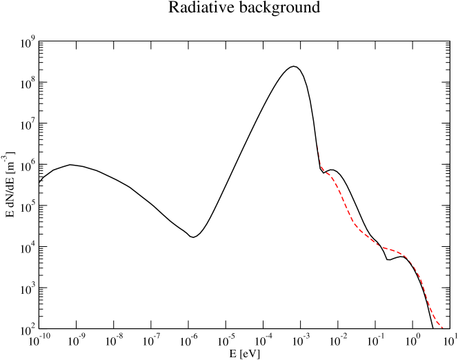
Figure 2: The local photon background we used. The main peak is due to the CMB, the radio background is taken from [33] in the hypothesis of red-shift evolving sources, the IR-UV background is taken from [24]. The dashed curve shows the result obtained in [30].

The local photon background obtained as a superposition of the IR-Optical-UV, the radio and the microwave background is plotted in fig. 2, where the dashed curve shows, for comparison, the result of Ref. [30]. We checked that our results do not change appreciably by changing the IR background, the reason being that most part of the cascade develops on the URB and on the CMB radiation.

4 The Electromagnetic cascade: a detailed calculation

In this section we describe our calculation of the electromagnetic cascade initiated by a proton with ultra-high energy through photopion production off the photons of the CMBR. In §4.1 we describe the calculation of the rate of injection of gamma rays and electrons in the cascade due to discrete interactions of photopion production. In §4.2 we describe in detail the propagation of electrons and gamma rays in the background radiation field.

4.1 Gamma rays and electrons from photopion production

At energies larger than the threshold for photopion production, given by

$$E_{th}=\frac{m_{\pi}^{2}+2m_{\pi}m_{p}}{4\epsilon},$$ (15)

where $\epsilon$ is the energy of the target photon, a proton can generate a pion in the final state, in the reaction of photopion production as written in Eq. 1. The decay of the $\pi^{0}$ or $\pi^{+}$ generates either gamma rays ($\pi^{0}\to\gamma\gamma$) or electrons ($\pi^{+}\to\mu^{+}\nu_{\mu};\leavevmode\nobreak\ \mu\to e+\nu_{\mu}+\nu_{e}$). Both these secondary products can initiate a cascade in the universal photon background calculated in the previous section.

The propagation of UHECRs from a source at a given distance is simulated using the Montecarlo approach presented in [4]. However, in the version of the simulation adopted here we improved the code by simulating the single proton-photon interactions using SOPHIA [34, 35]. This event generator treats an interaction either via baryon resonance excitation, one particle t-channel exchange (direct one-particle production), diffractive particle production and (non-diffractive) multiparticle production using string fragmentation. The distribution and momenta of the final state particles are calculated from their branching ratios and interaction kinematics in the center of mass frame, and the particle energies and angles in the lab frame are calculated by Lorentz transformations. SOPHIA takes care also of the decay of all unstable particles (except for neutrons) using standard Monte Carlo methods of particle decay according to the available phase space. The neutron decay is implemented separately due to its much longer lifetime. The SOPHIA event generator has been shown to be in good agreement with available accelerator data. A detailed description of the code including the sampling methods, the interaction physics used, and the performed tests can be found in Ref. [34].

The gamma ray and positron yields used in our calculation are computed by simply accounting for the decay of neutral and charged pions. The spectra of gamma rays at different distances from the source, for a given distance between the source and the observer are plotted in Fig. 3. The spectra of electrons/positrons coming from the decay of charged pions for the same distances from the source are shown in Fig. 4.

As shown in [4], the injection spectrum of UHECRs that best fits the observed data of AGASA and HiRes in the energy region below $10^{20}$ eV is a power law $E^{-\gamma}$ with $\gamma=2.6$ in the case of sources that do not have luminosity evolution with redshift. The injection spectrum flattens to $E^{-2.4}$ for the case of sources with strong luminosity evolution $L(z)\propto(1+z)^{4}$.

In [12] a detailed analysis of the consequence of small scale anisotropies in the directions of arrival of UHECRs was carried out. It was found there that the number of doublets and triplets observed by AGASA suggests that the sources of UHECRs are powerful relatively rare sources, with a typical number density $10^{-6}-10^{-5}\leavevmode\nobreak\ \rm Mpc^{-3}$ and a luminosity at energies above $10^{19}$ eV of $\sim 2\times 10^{42}-2\times 10^{43}\leavevmode\nobreak\ \rm erg\leavevmode\nobreak\ s^{-1}$.

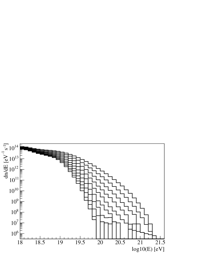
Figure 3: Photon injection spectra accumulated in bins of 10 Mpc width from the source (from top to bottom).

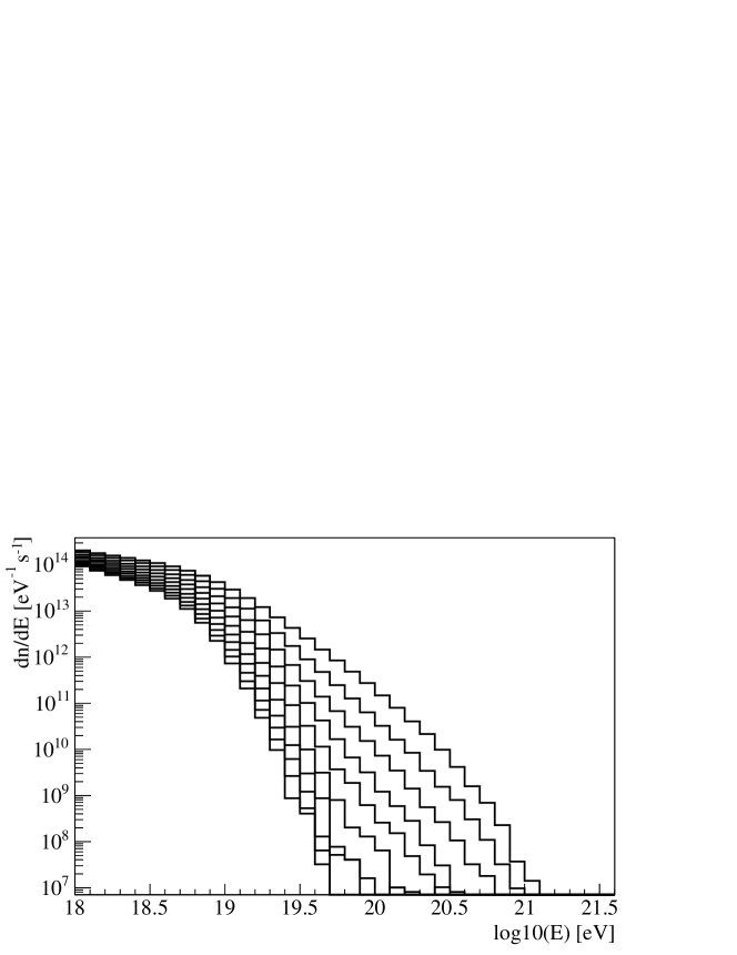
Figure 4: Positron injection spectra accumulated in bins of 10 Mpc width from the source (from top to bottom).

The reactions of photopion production during the propagation of UHECRs from the sources to the Earth generate at any time new gamma rays and electrons, that start new cascades that will eventually reach the Earth.

4.2 The development of the electromagnetic cascade

As already discussed at length in section 2, the electromagnetic cascade is mainly driven by Inverse Compton Scattering (ICS) of high energy electrons on the low energy background photons and Pair Production (PP) of high energy photons on the low energy background photons. Higher order QED processes become important only for energies exceeding $10^{21}{\,\rm eV}$ and have a significant impact only in the absence of magnetic fields and for a narrow peaked background spectrum [36]. In our calculations we only include ICS, PP and synchrotron emission in the presence of an intergalactic magnetic field.

Here we use the following notation: $f_{e}(E,t)$ is the differential spectrum of electrons at time $t$ during the evolution of the cascade, $f_{\gamma}(E,t)$ is the differential spectrum of photons at the same time $t$. We calculate these spectra by solving the coupled Boltzman equations that describe the evolution of $f_{e}$ and $f_{\gamma}$ due to energy losses.

The Boltzmann equations read [40]:

$$\frac{{\rm d}f_{e}(E,t)}{{\rm d}t}=-\int\mathrm{d}\epsilon n_{b}(\epsilon)R_{ICS}(E,\epsilon)f_{e}(E,t)+\\ \int\mathrm{d}\epsilon n_{b}(\epsilon)\int\mathrm{d}E^{\prime}P_{ICS,e}f_{e}(E^{\prime},t)+\int\mathrm{d}\epsilon n_{b}(\epsilon)\int\mathrm{d}E^{\prime}P_{PP}f_{\gamma}(E^{\prime},t)+q_{e}(E,t)$$ (16)

$$\frac{{\rm d}f_{\gamma}(E,t)}{{\rm d}t}=-\int\mathrm{d}\epsilon n_{b}(\epsilon)R_{PP}(E,\epsilon)f_{\gamma}(E,t)+\\ \int\mathrm{d}\epsilon n_{b}(\epsilon)\int\mathrm{d}E^{\prime}P_{ICS,\gamma}f_{e}(E^{\prime},t)+q_{\gamma}(E,t),$$ (17)

where we introduced the angle averaged cross sections as

$$R(E,\epsilon)=\int_{-1}^{1}\mathrm{d}\mu\frac{1-\mu\beta_{e,\gamma}}{2}\sigma(s(\epsilon_{b},E,\mu))$$ (18)

and the angle averaged differential cross sections as

$$P(E^{\prime};E,\epsilon)=\int_{-1}^{1}\mathrm{d}\mu\frac{1-\mu\beta_{e,\gamma}}{2}\frac{{\rm d}\sigma(s(\epsilon_{b},E,\mu))}{{\rm d}E^{\prime}}.$$ (19)

Here $s(\epsilon_{b},E,\mu)$ is the center of mass squared energy for a particle with energy $E$ scattering a photon with energy $\epsilon_{b}$ at angle having cosine $\mu$. $n_{b}(\epsilon)$ is the spectrum of background photons. $q_{e}(E,t)$ and $q_{\gamma}(E,t)$ are the source functions for electrons and photons respectively, calculated as described in §4.1. At any time new electrons and gamma rays are generated and start new cascades, due to the reactions of photopion production of protons.

4.2.1 Pair production

The pair production cross section is given by [37]:

$$\sigma_{PP}=\sigma_{T}\frac{3}{16}\left(1-\beta^{2}\right)\left[\left(3-\beta^{4}\right)\ln\frac{1+\beta}{1-\beta}-2\beta\left(2-\beta\right)\right],$$ (20)

where $\beta$ is the velocity of the outgoing electron in the Center of Mass (CM) frame.

The threshold for pair production is:

$$E_{th}=\frac{m_{E}^{2}}{\epsilon}\simeq 2.6\times 10^{11}\left(\frac{\epsilon}{{\,\rm eV}}\right)^{-1}{\,\rm eV}.$$ (21)

The spectrum of electrons generated by pair production in the interaction of two photons with energy $E_{\gamma}$ and $\epsilon_{\gamma}$ with $E_{\gamma}\gg\epsilon_{\gamma}$ is [38]:

$$\frac{{\rm d}N_{e}}{{\rm d}E^{\prime}_{e}}\left(E_{\gamma},\epsilon,E^{\prime}_{e}\right)=\sigma_{T}\frac{3}{64}\frac{1}{\epsilon^{2}E_{\gamma}^{3}}\left[\frac{4A}{(A-E_{e}^{\prime})E_{e}^{\prime}}\log\left(4\epsilon(A-E_{e}^{\prime})\frac{E_{e}^{\prime}}{A}\right)-8\epsilon A+\right.\\ \left.2(2\epsilon A-1)\frac{A^{2}}{(A-E_{e}^{\prime})E_{e}^{\prime}}+-\left(1-\frac{1}{\epsilon A}\right)\frac{A^{4}}{(A-E_{e}^{\prime})^{2}E_{e}^{\prime 2}}\right]$$ (22)

where all energies are in units of the electron mass and we put $A=\epsilon+E_{\gamma}$. The range of electron energies in the final state is defined by:

$$\frac{A}{2}\left(1-\sqrt{1-\frac{1}{E\epsilon}}\right)\leq E^{\prime}_{e}\leq\frac{A}{2}\left(1+\sqrt{1-\frac{1}{E\epsilon}}\right).$$ (23)

4.2.2 Inverse Compton Scattering

The cross section for ICS ($e\gamma_{b}\rightarrow e\gamma$) is given by the well-known Klein-Nishina expression (e.g.[39, 40]):

$$\sigma_{\rm ICS}=\sigma_{T}\cdot\frac{3}{8}\frac{m_{e}^{2}}{s\beta}\left[\frac{2}{\beta(1+\beta)}(2+2\beta-\beta^{2}-2\beta^{3})-\frac{1}{\beta^{2}}(2-3\beta^{2}-\beta^{3})\ln\frac{1+\beta}{1-\beta}\right],$$ (24)

where $\beta\equiv(s-m_{e}^{2})/(s+m_{e}^{2})$ is the velocity of the outgoing electron in the center of mass frame.

As in the case of pair production, we use an approximate formula for the spectrum of the produced photons/electrons. The approximation holds as long as the incoming electron is relativistic. The spectrum of electrons resulting from the scattering is [41, 42]:

$$\frac{{\rm d}N_{\gamma}}{{\rm d}E^{\prime}_{\gamma}}\left(E_{e},\epsilon,E^{\prime}_{\gamma}\right)=\sigma_{T}\frac{3}{4\gamma\epsilon}\left[2q+\log q+(1+2q)(1-q)+\frac{1}{2}\left(\Gamma_{e}q\right)^{2}\frac{1-q}{1+\Gamma_{e}q}\right],$$ (25)

where $\gamma=\sqrt{1+E_{e}^{2}}$, $E_{1}=E_{\gamma}^{\prime}/\gamma$, $\Gamma_{e}=4\epsilon\gamma$, $q=\frac{E_{1}}{\Gamma_{e}(1-E_{1})}$ and the range is restricted to $\frac{\epsilon}{E_{e}}\leq E_{1}\leq\frac{\Gamma_{e}}{1+\Gamma_{e}}$. All energies are again in units of the electron mass.

The differential spectrum of the outgoing photons is obtained by substituting $E_{e}-E^{\prime}_{e}$ to $E^{\prime}_{\gamma}$ in eq. (25).

By averaging the spectra of equations (22) and (25) over the background spectrum we can obtain directly the integrated quantities of Eq. (17):

$$\int\mathrm{d}\epsilon n(\epsilon)P_{PP}(E_{e}^{\prime};E_{\gamma},\epsilon)=\int\mathrm{d}\epsilon n(\epsilon)\frac{{\rm d}N_{e}}{{\rm d}E^{\prime}_{e}}\left(E_{\gamma},\epsilon,E^{\prime}_{e}\right)$$ (26)

and

$$\int\mathrm{d}\epsilon n(\epsilon)P_{ICS,\gamma}(E_{\gamma}^{\prime};E_{e},\epsilon)=\int\mathrm{d}\epsilon n(\epsilon)\frac{{\rm d}N_{\gamma}}{{\rm d}E^{\prime}_{e}}\left(E_{e},\epsilon,E^{\prime}_{\gamma}\right)$$ (27)

and similarly for the outgoing electrons.

4.2.3 The magnetic field

Synchrotron losses of high energy electrons are introduced as continuous energy losses. This works perfectly for the range of energies that we are interested in.

The rate of energy losses can be written as:

$$\frac{{\rm d}E_{e}}{{\rm d}t}=-\frac{4}{3}c\sigma_{T}\frac{B^{2}}{8\pi}\left(\frac{E}{m_{e}c^{2}}\right)^{2}\mathinner{\langle{\sin\alpha}\rangle}\simeq 7.9\times 10^{-17}\mathinner{\langle{\sin\alpha}\rangle}\left(\frac{B}{\mathrm{nG}}\right)^{2}\left(\frac{E}{\,{\rm GeV}}\right)^{2}\frac{\,{\rm GeV}}{\mathrm{year}}$$ (28)

where $\alpha$ is a pitch angle.

The spectrum of photons radiated by synchrotron emission by an electron with energy $E$, assuming isotropy of the electron distribution, is [39]

$$\frac{{\rm d}P}{{\rm d}E^{\prime}}=\frac{2\sqrt{3}}{3}\mu_{B}B\alpha\hbar F\left(\frac{E^{\prime}}{E_{C}}\right)$$ (29)

where $\mu_{B}=9.27\times 10^{-21}$ erg/G is the Bohr magneton, $\alpha$ is the fine structure constant,

$$E_{C}=3\mu_{B}B\gamma^{2}\simeq 6.6\times 10^{-20}\frac{B}{\mathrm{nG}}\left(\frac{E}{\,{\rm GeV}}\right)^{2}\,{\rm GeV}$$ (30)

is the critical energy and

$$F(x)=x\int_{x}^{\infty}K_{5/3}(\xi)\mathrm{d}\xi$$ (31)

with $K_{5/3}(\xi)$ the modified Bessel function of fractional order. The power spectrum peaks at $E_{\gamma}\simeq 0.29E_{c}$.

5 Results

In this section we discuss the results of our numerical calculations of the development of the electromagnetic cascade from nearby sources of UHECRs. We first discuss the case in which the cascade develops in the absence of magnetic field in the intergalactic medium (§5.1). In §5.2 we apply our calculations to a magnetized universe.

5.1 The unmagnetized case

Numerical calculations of the propagation of UHECRs from point sources appear to give small scale anisotropies compatible with the observations carried out with the AGASA experiment for a source density of $10^{-6}-10^{-5}\leavevmode\nobreak\ \rm Mpc^{-3}$, corresponding to a source luminosity above $10^{19}$ eV of $2\times 10^{43}-2\times 10^{42}\rm erg\,s^{-1}$. The best fit injection spectrum is $E^{-2.6}$ for sources with no luminosity evolution and $E^{-2.4}$ for sources with strong luminosity evolution, $L(z)\propto(1+z)^{4}$. We followed the propagation of UHECRs with the simulation used in [4, 12] in which the interactions are implemented with the SOPHIA package. At each step of the simulation, the spectra of gamma rays (from the decay of neutral pions) and of electrons (from the decay of charged pions) are determined and used as source functions for the gamma rays and electrons respectively in the coupled Boltzmann equations for the development of the electromagnetic cascade.

The results of our calculations for a proton injection spectrum $E^{-2.6}$ are shown in Fig. 5 for a source located at 6 Mpc (short dashed line), 21 Mpc (solid line), 48 Mpc (long dashed line) and 71 Mpc (dash-dotted line). In the same plot we show the sensitivities of MAGIC, HESS, VERITAS and GLAST (thick lines).

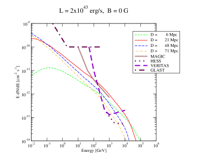
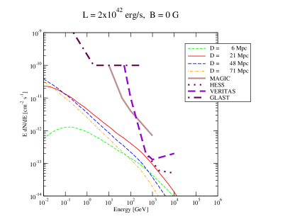
Figure 5: Flux of gamma ray at the Earth as resulting from the injection of cosmic rays in continuous point sources located at the distances indicated in the graph. The thick lines are the sensitivities of MAGIC, HESS, VERITAS and GLAST. The left (right) panel is for a source with luminosity $2\times 10^{43}\leavevmode\nobreak\ \rm erg\,s^{-1}$ ($2\times 10^{42}\leavevmode\nobreak\ \rm erg\,s^{-1}$) at energies larger than $10^{19}$ eV.

For the case with higher luminosity (left panel) the predicted fluxes should be detectable by the experiments HESS and VERITAS for all the considered distances. MAGIC should detect a signal only if the source is at about 20 Mpc distance. The corresponding fluxes for the case with source luminosity $2\times 10^{42}\leavevmode\nobreak\ \rm ergs^{-1}$ are slightly below the sensitivities of these telescopes. None of the predicted fluxes appears to be detectable in the lower energy range, accessible to GLAST. It is worth to remind that the largest distance considered in the calculations is comparable with the loss length of UHECRs with energy in excess of $10^{20}$ eV, for which a counterpart is still lacking.

The flux of gamma rays does not necessarily decrease for larger distances to the source. This is due to the fact that for too small distances, the electromagnetic cascade has not enough time to develop and the lower energy part of the spectrum does not reach the equilibrium shape. This is the reason why in Fig. 5 the spectrum of gamma rays from a source at distance 6 Mpc (short dashed line) for a wide range of energies is below that corresponding to a source at larger distances.

Another point to keep in mind is that the calculation in [12] were carried out for a class of sources with identical luminosity. It would probably be more realistic to imagine that the sources of UHECRs have some kind of luminosity function, and that the value used here is some sort of average luminosity. In this case it is quite plausible that sources with cosmic ray luminosity larger than $2\times 10^{43}\leavevmode\nobreak\ \rm erg\leavevmode\nobreak\ s^{-1}$ exist in nature. Since the flux of gamma rays in the cascade scales linearly with the cosmic ray luminosity, the cascade signal increases correspondingly.

For sources with a strong luminosity evolution, the flatter required injection spectrum in the form of UHECRs slightly increases the predicted cascade fluxes, as shown in Fig. 6.

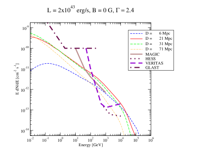
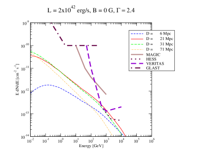
Figure 6: Flux of gamma ray at the Earth as resulting from the injection of cosmic rays in continuous point sources located at the distances indicated in the graph. The thick lines are the sensitivities of MAGIC, HESS, VERITAS and GLAST. The left (right) panel is for a source with luminosity $2\times 10^{43}\leavevmode\nobreak\ \rm erg\,s^{-1}$ ($2\times 10^{42}\leavevmode\nobreak\ \rm erg\,s^{-1}$) at energies larger than $10^{19}$ eV. The luminosity evolution of the sources is taken as $L(z)\propto(1+z)^{4}$ and the injection spectrum of UHECRs as $E^{-2.4}$.

5.2 The case of a magnetized universe

The development of electromagnetic cascades in the universe is very sensitive to the presence of magnetic fields, mainly in two ways: 1) the presence of a magnetic field modifies the duration of the cascading processes as observed at the Earth, due to the deflection of the charged components in the cascade; 2) electrons with very high energy can lose energy by synchrotron emission, therefore subtracting energy from the cascade.

The first effect is important only for the case of bursting sources. In that case the duration of the burst in the form of the electromagnetic cascade may depend on energy, namely the duration of the burst appears to be different at different energies. Very tight limits on the magnetic field in the IGM can be imposed in principle from the detection or non detection of the lowest energy part of the cascade [43]. Since we consider here continuous sources, we will not investigate any further this first effect of the magnetic field, and we will concentrate our attention on the role of synchrotron losses of the electron component.

At very high energies, the cross section for ICS is in the Klein-Nishina regime. This is the energy region where it is easier for the synchrotron losses to dominate over ICS. Therefore we expect that the role of the magnetic field is particularly relevant when the field is concentrated around the source, where the electrons in the cascade have the highest energies. Moreover, as discussed in §4.2.3, synchrotron losses may become dominant on ICS in the energy region around $10^{20}$ eV if the field is larger than $\sim 10^{-10}$ G.

Our results for the case of a source with luminosity $2\times 10^{43}\leavevmode\nobreak\ \rm erg\leavevmode\nobreak\ s^{-1}$ are summarized in Fig. 7 for four values of the magnetic field, namely $10^{-11}$ G, $10^{-10}$ G, $10^{-9}$ G and $10^{-8}$ G. The distances to the source are taken as in Fig. 5, while the source luminosity in the form of cosmic rays with energy above $10^{19}$ eV has been taken to be $2\times 10^{43}\leavevmode\nobreak\ \rm erg\leavevmode\nobreak\ s^{-1}$.

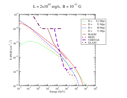
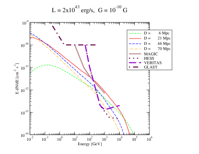
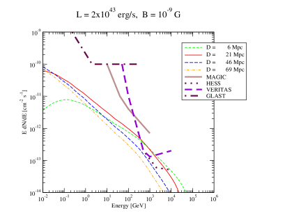
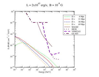
Figure 7: Flux of gamma rays at the Earth for a magnetic field in the intergalactic medium $B=10^{-11},10^{-10},10^{-9},10^{-8}$ Gauss and a source with luminosity $2\times 10^{43}\leavevmode\nobreak\ \rm erg\,s^{-1}$ at energies larger than $10^{19}$ eV.

The effect of the magnetic field on the development of the electromagnetic cascade is clear: for magnetic fields smaller than $10^{-9}$ G the predicted fluxes start to be at the level of sensitivity of VERITAS and HESS, and are undetectable for larger magnetic field strengths. On the other hand, one has to keep in mind that a magnetic field of $10^{-9}$ G widespread in the whole IGM is already the highest possible value compatible with Faraday rotation measurements [44]. Larger fields are possible only on more compact regions: for this reason we also explore the situation in which a magnetic field is present only in a neighborhood of the source or near the Earth. A recent investigation of the effects of this magnetic field on the propagation of UHECRs has been presented in [45, 46]. In particular in Ref. [45] it was shown that the average magnetic fields are quite smaller that $10^{-9}$ G, with the exception of the filamentary regions where they are of the order of $10^{-9}$ G. Clearly much higher fields are achieved in Mpc scale virialized regions such as clusters of galaxies. This conclusion does not appear to be confirmed in [46].

In the left panel of Fig. 8 we plot the fluxes of gamma rays calculated if the source is located in a region of 10 Mpc where the magnetic field is $10^{-9}$ G.

Similarly, in the right panel of Fig. 8 we plot the fluxes of gamma rays calculated in the case that the Earth is located in a region of 10 Mpc in which the field is $10^{-9}$ G. This might be the case for the Local Supercluster.

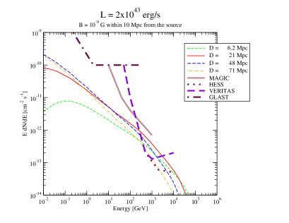
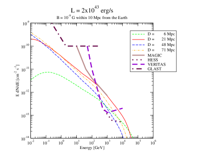
Figure 8: Flux of gamma rays at the Earth for a magnetic field in the intergalactic medium $B=10^{-9}$ Gauss located in a region of 10 Mpc around the source and the Earth respectively. The source luminosity is $2\times 10^{43}\leavevmode\nobreak\ \rm erg\,s^{-1}$ at energies larger than $10^{19}$ eV.

It is easy to see that if the magnetic field is concentrated close to the detector and not close to the source, its effect on the development of the cascade is negligible, as can be inferred by comparing the right panel of Fig. 8 and the left panel of Fig. 5.

In the left (right) panel of Fig. 9 we plot the expected fluxes in the case that the magnetic field is $10^{-8}$ G in a region of size $1$ Mpc around the source (Earth). The expected fluxes in these cases are not much affected by the presence of the magnetic field: in the near source region of 1 Mpc almost no reaction of photopion production occurred, therefore no cascade was developed yet. In the near Earth region the cascade has already reached in most cases the final stages, where the effects of synchrotron losses of electrons are irrelevant compared with ICS.

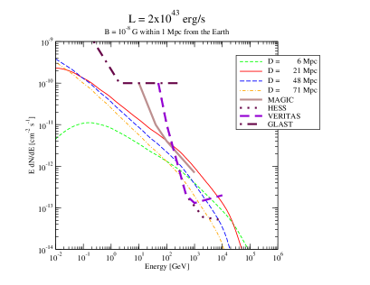
Figure 9: Flux of gamma rays at the Earth for a magnetic field in the intergalactic medium $B=10^{-8}$ Gauss located in a region of 1 Mpc around the source and around the Earth respectively. The source luminosity is $2\times 10^{43}\leavevmode\nobreak\ \rm erg\,s^{-1}$ at energies larger than $10^{19}$ eV.

6 Conclusions

The sources of UHECRs are still unknown mainly because we do not know yet whether they are generated in a few very powerful sources or rather in numerous low power sources. This degeneracy has probably been broken after the discovery of small scale anisotropies in the arrival directions of UHECRs in the AGASA experiment, although the statistical significance of this discovery appears to be still controversial [10]. In [12], the AGASA data were used to infer that the most likely number density of sources of UHECRs is around $10^{-6}-10^{-5}\leavevmode\nobreak\ \rm Mpc^{-3}$, which corresponds to a source luminosity of $2\times 10^{43}-2\times 10^{42}\leavevmode\nobreak\ \rm erg\leavevmode\nobreak\ s^{-1}$ at energies above $10^{19}$ eV. These estimates, obtained in the absence of intergalactic magnetic fields, remain valid as long as the magnetic field does not exceed $\sim 10^{-10}$ G over cosmological distances.

During their propagation from the sources to the Earth UHECRs suffer photopion production if their energy is above threshold for this process, therefore generating charged and neutral pions. While the former decay mainly into electrons and neutrinos, the latter generate gamma rays. Both gamma rays and electrons initiate an electromagnetic cascade that transfers energy from high energies to lower energies, more easily accessible to gamma ray telescopes. We calculated the development of this electromagnetic cascade with and without the presence of an intergalactic magnetic field, and investigated the detectability of the gamma ray signal with ground based telescopes such as MAGIC, VERITAS and HESS, as well as with space-borne telescopes such as GLAST .

The cascade radiation appears to be detectable by VERITAS and HESS for a source luminosity around $2\times 10^{43}\leavevmode\nobreak\ \rm erg\leavevmode\nobreak\ s^{-1}$ in the form of cosmic rays with energy larger than $10^{19}$ eV, if the magnetic field in the IGM is constant over all the propagation volume and smaller than $10^{-9}$ G (This luminosity corresponds to the lower source density compatible with the small scale anisotropies observed by AGASA). If the magnetic field is patched, stronger fields are allowed close to the Earth without appreciably changing the previous conclusions. If the region with stronger fields is close to the source location, the initial stages of the cascade may be affected if the magnetized region is large enough, so that the energy content of the cascade gets suppressed. A large field close to the Earth does not affect the conclusions in any appreciable way, since the cascade is already fully developed at that point. A magnetic field of 1nG near the source implies slightly lower gamma ray fluxes if it is extended in a region of about 10 Mpc. A stronger field, of say 10 nG, in a 1 Mpc region either around the source or the observer does not change the results in any appreciable way.

The main uncertainty involved in our calculations is the luminosity of the sources in the form of UHECRs. The numbers we adopted are derived in [12], on the basis of the appearance of small scale anisotropies in the AGASA data and in the assumption of sources that accelerate UHECRs continuously. For bursting sources, the luminosity per source may be many orders of magnitude larger than that adopted here, but it would be concentrated within a short time interval. The diffuse and time-spread appearance of the observed UHECRs is achieved, within this class of models, by assuming the presence of a small magnetic field in the intergalactic medium, responsible for sizeable time delay that make the burst look like a continuous signal when observed through charged particles. This is the case for the gamma ray burst models [47, 48, 49] of UHECRs.

A similar time delay is introduced in the development of the electromagnetic cascade. Moreover, an additional time delay is introduced due to the presence of electrons and positrons in the cascade itself. These effects cannot be accounted for within the framework proposed here, and will be considered in a forthcoming publication.

References

- [1] A. A. Penzias and R. W. Wilson, ApJ 146, 666 (1966).
- [2] K. Greisen, Phys. Rev. Lett. 16, 748 (1966).
- [3] G. T. Zatsepin and V. A. Kuzmin, Sov. Phys. JETP Lett. 4, 78 (1966).
- [4] D. De Marco, P. Blasi, and A. V. Olinto, Astroparticle Physics 20, 53 (2003).
- [5] P. G. Tinyakov and I. I. Tkachev, Astroparticle Physics 18, 165 (2002).
- [6] D. S. Gorbunov, P. G. Tinyakov, I. I. Tkachev, and S. V. Troitsky, ApJ 577, L93 (2002).
- [7] N.W. Evans, F. Ferrer, S. Sarkar, Phys. Rev. D 67, 103005 (2003).
- [8] P. Tinyakov, and I. Tkachev, preprint astro-ph/0301336.
- [9] Y. Uchihori et al., Astroparticle Physics 13, 151 (2000).
- [10] C. B. Finley and S. Westerhoff, preprint astro-ph/0309159 .
- [11] D. Harari, S. Mollerach, and E. Roulet, Journal of High Energy Physics 2, 35 (2000).
- [12] P. Blasi and D. De Marco, Astroparticle Physics in press, preprint astro-ph/0307067 (2003).
- [13] W. S. Burgett and M. R. O’Malley, Phys. Rev. D 67, 92002 (2003).
- [14] H. Goldberg and T. J. Weiler, Phys. Rev. D 64, 56008 (2001).
- [15] S. L. Dubovsky, P. G. Tinyakov, and I. I. Tkachev, Physical Review Letters 85, 1154 (2000).
- [16] Z. Fodor and S. D. Katz, Phys. Rev. D 63, 23002 (2001).
- [17] H. Yoshiguchi, S. Nagataki, S. Tsubaki, K. Sato, ApJ 586, 1211 (2003).
- [18] G. Sigl, F. Miniati, T. Ensslin, Phys. Rev. D68, 043002 (2003).
- [19] V. S. Berezinskii and A. I. Smirnov, Ap&SS 32, 461 (1975).
- [20] V. L. Ginzburg, V. A. Dogiel, V. S. Berezinsky, S. V. Bulanov, and V. S. Ptuskin, Astrophysics of cosmic rays, Amsterdam, Netherlands: North-Holland 534 p., 1990.
- [21] D. J. Fixsen et al., ApJ 473, 576 (1996).
- [22] D. Elbaz et al., A&A 384, 848 (2002).
- [23] J. A. Peacock, Cosmological physics, Cambridge, UK: Cambridge University Press, 1999.
- [24] R. Chary and D. Elbaz, ApJ 556, 562 (2001).
- [25] D. N. Spergel et al., ApJS 148, 175 (2003).
- [26] G. L. Granato et al., Ap&SS 276, 973 (2001).
- [27] C. Xu, ApJ 541, 134 (2000).
- [28] C. Xu et al., ApJ 508, 576 (1998).
- [29] E. Dwek and M. K. Barker, ApJ 575, 7 (2002).
- [30] O. C. de Jager and F. W. Stecker, ApJ 566, 738 (2002).
- [31] J. K. Alexander, L. W. Brown, T. A. Clark, R. G. Stone, and R. R. Weber, ApJ 157, L163+ (1969).
- [32] V. S. Berezinsky, Yad. Fiz 11, 339 (1970).
- [33] R. J. Protheroe and P. L. Biermann, Astroparticle Physics 6, 45 (1996).
- [34] A. Mucke, R. Engel, J. P. Rachen, R. J. Protheroe, and T. Stanev, Comput. Phys. Commun. 124, 290 (2000).
- [35] T. Stanev, R. Engel, A. Mucke, R. J. Protheroe, and J. P. Rachen, Phys. Rev. D62, 093005 (2000).
- [36] P. Bhattacharjee and G. Sigl, Phys. Rep. 327, 109 (2000).
- [37] R. Svensson, ApJ 258, 321 (1982).
- [38] F. A. Agaronyan, A. M. Atoyan, and A. M. Nagapetyan, Astrophysics 19, 187 (1983).
- [39] G. B. Rybicki and A. P. Lightman, Radiative processes in astrophysics, New York: Wiley-Interscience, 393 p., 1979.
- [40] S. Lee, Phys. Rev. D 58, 43004 (1998).
- [41] G. R. Blumenthal and R. J. Gould, Reviews of Modern Physics 42, 237 (1970).
- [42] F. C. Jones, Physical Review 167, 1159 (1968).
- [43] Z. G. Dai, B. Zhang, L. J. Gou, P. Mészáros, and E. Waxman, ApJ 580, L7 (2002).
- [44] P. Blasi, S. Burles, and A. Olinto, ApJ 514, 79 (1999).
- [45] K. Dolag, D. Grasso, V. Springel and I. Tkachev, preprint astro-ph/0310902.
- [46] G. Sigl, F. Miniati, and T. Ensslin, preprint astro-ph/0309695.
- [47] M. Vietri, ApJ 453, 883 (1995).
- [48] E. Waxman, ApJ 452, 1 (1995).
- [49] M. Vietri, D. De Marco, and D. Guetta, ApJ 592, 378 (2003).