Shear Selected Cluster Cosmology: Tomography and Optimal Filtering

Abstract

We study the potential of weak lensing surveys to detect clusters of galaxies, using a fast Particle Mesh cosmological N-body simulation algorithm specifically tailored to investigate the statistics of these shear selected clusters. In particular, we explore the degree to which the radial positions of galaxy clusters can be determined tomographically, by using photometric redshifts of background source galaxies. We quantify the errors in the tomographic redshifts, $\Delta z\equiv z_{\rm tomography}-z_{\rm real}$, and study their dependence on mass, redshift, detection significance, and filtering scheme. For clusters detected with signal to noise ratio $S/N\gtrsim 4.5$, the fraction of clusters with tomographic redshift errors $|\Delta z|\leq 0.2$ is $45\%$ and the root mean square deviation from the real redshifts is $\langle(\Delta z)^{2}\rangle^{1/2}=0.41$, with smaller errors for higher $S/N$ ratios. A Tomographic Matched Filtering (TMF) scheme, which combines tomography and matched filtering, is introduced which optimally detects clusters of galaxies in weak lensing surveys. The TMF exploits the extra information provided by photometric redshifts of background source galaxies, neglected in previous studies, to optimally weight the sources. The efficacy and reliability of the TMF is investigated using a large ensemble of mock observations from our simulations and detailed comparisons are made to other filters. Using photometric redshift information with the TMF enhances the number of clusters detected with $S/N\gtrsim 4.5$ by as much as $76\%$, and it increases the dynamic range of weak lensing searches for clusters, detecting more high redshift clusters and extending the mass sensitivity down to the scale of large groups. Furthermore, we find that coarse redshift binning of source galaxies with as few as three bins is sufficient to realize the gains of the TMF. Thus, the tomographic filtering techniques presented here can be applied to current ground based weak lensing data in as few as three bands, since two colors and magnitude prior are sufficient to bin source galaxies this coarsely. Cosmological applications of shear selected cluster samples are also discussed.

1. Introduction

Mapping the distribution of dark matter in the universe is now one of the primary goals of observational cosmology. The traditional approach has been to survey the sky for a population of luminous objects, assuming a direct relationship between luminosity and dark matter. While large galaxy surveys such as the 2dF Galaxy Redshift Survey (Colless et al. 2001) and the Sloan Digital Sky Survey (York et al. 2000) are perhaps the first examples that come to mind, future wide field X-ray (Romer et al. 2001) and Sunyaev-Z’eldovich (SZ) surveys (Carlstrom, Holder, & Reese 2002; Kosowsky 2003) will usher in an era where maps of the universe will be available at multiple frequencies. Generically, all objects that emit radiation will be biased tracers of the underlying dark matter distribution. Hence, the interpretation of this data is limited by our ability to quantify the relationship between dark and luminous matter.

Weak gravitational lensing, or the coherent distortion of images of faint background galaxies by the foreground matter distribution, provides a unique opportunity to map the dark matter directly without making any assumptions about how baryons trace dark matter (see e.g., Bartelmann & Schneider (2001) or Van Waerbeke & Mellier (2003) for a review). Recently, weak lensing by large scale structure, or “cosmic shear”, has been independently detected by several groups (see Table 1 of Van Waerbeke & Mellier (2003) for a compilation of references). The primary focus of these observations has been to measure the two point statistical properties of the shear field, which probes the matter power spectrum in projection. However, as first suggested by Kaiser (1995) and Schneider (1996), weak lensing surveys can also be used to detect individual mass concentrations, allowing one to construct a shear selected sample of dark halos. Typically these will be galaxy cluster size $M\gtrsim 10^{13.5}\ {\rm\ M}_{\odot}$ objects, as the finite number of background sources and their intrinsic ellipticity place a lower limit on the size of a halo that can be detected. To date, there are only two such cases of spectroscopically confirmed cluster detections from ‘blank field’ weak lensing observations (Wittman et al. 2001, 2003). Although, recently Schirmer et al. (2003, 2004) have used weak lensing to confirm several color-selected optical cluster candidates.

A shear selected sample of galaxy clusters would be of great astrophysical and cosmological interest. Probable biases in optical, X-ray, and SZ selected cluster samples with respect to richness, baryon fraction, morphology, and dynamical state, would be revealed (Hughes et al. 2004). Furthermore, if there does exist a population of high mass to light clusters that has hitherto gone undetected, this would cast serious doubt upon the “fair sample” hypotheses (White et al. 1993), invoked to determine the matter density parameter, $\Omega_{\rm m}$, from comparisons of cluster baryon fraction to total cluster mass measurements (see e.g., Allen, Schmidt, & Bridle (2003) or Voevodkin & Vikhlinin (2004) for recent examples).

Perhaps a more contentious issue is the possible existence of a population of truly dark clusters. Recently, several groups have purportedly detected dark mass concentrations from weak lensing (Fischer 1999; Erben et al. 2000; Umetsu & Futamase 2000; Miralles et al. 2002; Dahle et al. 2003, though see Erben et al. 2003). If these objects are actually ‘dark’ virialized mass concentrations as opposed to non-virialized objects (Weinberg & Kamionkowski 2002) or projections of large scale structure (Metzler, White, & Loken 2001; White, van Waerbeke, & Mackey 2002; Padmanabhan, Seljak, & Pen 2003; Hamana, Takada, & Yoshida 2003), this would pose serious challenges for our current structure formation paradigm and theories of galaxy formation. The absence of galaxies would require a complex form of feedback that suppresses galaxy formation in clusters. If such a dark cluster were X-ray or SZ faint, one would have to invoke some exotic mechanism to segregate dark matter from baryons on Mpc scales.

It is well known that a large sample of clusters of galaxies out to moderate redshift $z\sim 0.5$ can be used to impose stringent constraints on cosmological parameters. Several authors have recently suggested using the number count distribution of galaxy clusters, from X-ray and SZ observations (Haiman, Mohr, & Holder 2001; Weller & Battye 2003), deep optical surveys (Newman et al. 2002), and weak lensing (Bartelmann, Perrotta, & Baccigalupi 2002; Weinberg & Kamionkowski 2003), to probe the nature of the dark energy believed to be causing the acceleration of the expansion of the universe. Besides probing the dark energy, these cluster samples would constrain the matter density and amplitude of mass fluctuations (see e.g., Bahcall & Fan 1998; Holder, Haiman, & Mohr 2001; Pierpaoli, Borgani, Scott, & White 2003). In addition, the clustering of such cluster samples would provide another means to measure the matter power spectrum (Tadros, Efstathiou, & Dalton 1998; Schuecker et al. 2001) which would provide complimentary parameter constraints (Majumdar & Mohr 2003) and might possibly allow for a measurement of the angular diameter distance-redshift relation (Cooray et al. 2001) or baryon wiggles (Hu & Haiman 2003).

Yet, a limitation of the ‘baryon selection’ in optical, X-ray, and SZ cluster samples, is that their selection function depends on observables (e.g., richness, velocity dispersion, flux, temperature, SZ decrement) that serve as a proxy for mass. Attempts to model these mass-observable relationships depend on the uncertain astrophysics of galaxy formation and the state of baryons in clusters. While these can be determined empirically, scatter in the correlation between any two such observables is significant (see e.g., Kochanek et al. 2003); furthermore, these mass-observable relations surely evolve with redshift. The mass function of galaxy clusters is steep and exponentially sensitive to changes in limiting mass; moreover, errors in the mass-observable relations mimic cosmological parameter changes (Viana & Liddle 1999; Levine, Schulz, & White 2002; Majumdar & Mohr 2003; Hu 2003). Inclusion of uncertainties in the mass-observable relations significantly degrades constraints on cosmological parameters obtained from surveys that rely on a baryonic proxy for mass (Levine, Schulz, & White 2002; Majumdar & Mohr 2003). Although consistency checks provide additional leverage (Hu 2003), expensive follow up mass measurements are in general required to empirically calibrate the relationships between light and mass (Majumdar & Mohr 2003a; though see Lima & Hu 2004).

In this regard, the great advantage of a shear selected sample of galaxy clusters is that the selection function can be predicted ab initio, given a model for structure formation. Because on the scales of interest for weak lensing, only gravity is involved and the mass is dominated by dark matter, precision cosmological measurements will in principle be limited by instrumental systematics rather than unknown astrophysics. An accurate determination of the statistics of shear selected clusters from weak lensing requires N-body simulations of cosmological structure formation (though see Kruse & Schneider 1999; Bartelmann, Perrotta, & Baccigalupi 2002; Weinberg & Kamionkowski 2003, for simple analytical treatments), which brings us to the subject of this work.

In this paper we consider the detection of shear selected clusters using fast Particle Mesh (PM) N-body simulations of cosmological structure formation specifically tailored to investigate the statistics of weak lensing by clusters. Similar numerical studies carried out by other groups (Reblinsky et al. 1999; White, van Waerbeke, & Mackey 2002; Padmanabhan, Seljak, & Pen 2003; Hamana, Takada, & Yoshida 2003), have focused on the completeness and efficiency of weak lensing cluster searches. Devising an optimal filtering scheme to detect clusters has received little attention and furthermore, the additional information provided by photometric redshifts of background source galaxies has been neglected. In this paper we introduce the fast PM simulation algorithm, deduce the optimal cluster detection strategy, and investigate cluster tomography.

A fundamental obstacle for weak lensing studies of the matter distribution is the lack of radial information. All of the matter along the line-of-sight to a distant source contributes to the lensing and so the distortion reflects a two dimensional projection of the dark matter. This limitation can be overcome by using photometric redshifts of the background source population, which will be distributed in redshift, thus allowing for a tomographic reconstruction of the three dimensional foreground matter distribution.

A variant of this technique has already been applied to real weak lensing data. Wittman et al. (2001, 2003) tomographically determined the redshifts of two shear selected clusters at $z_{\rm d}=0.30$ and $z_{\rm d}=0.70$ respectively, which were both confirmed by follow up spectroscopy to be at $z=0.28$ and $z=0.68$. Recently, Taylor et al. (2004) conducted a weak lensing analysis of the previously known Abell supercluster A901/2 at $z=0.16$, and tomographically confirmed its redshift from weak lensing alone. They even constructed the first 3-D map of the dark matter potential of this cluster using the inversion method introduced by Taylor (2001). Hu & Keeton (2002) and Bacon & Taylor (2003) applied the Taylor (2001) tomographic inversion method to analytical models of clusters put in ‘by hand’, with mixed success. However, the reliability of these tomographic reconstruction techniques have yet to be characterized on realistic distributions of matter from N-body simulations; although it is clear that the fidelity of the reconstructions will be severely degraded by line of sight projections of large scale structure.

In this work we introduce a complementary tomographic technique which is effectively two dimensional. It is qualitatively similar to that used by Wittman et al. (2001, 2003) and Taylor et al. (2004) and also to maximum likelihood methods developed to study cluster mass profiles (Geiger & Schneider 1998; Schneider, King, & Erben 2000; King & Schneider 2001). The efficacy and reliability of the method is investigated by applying it to our large ensemble of N-body simulations. Additionally, a Tomographic Matched Filtering (TMF) scheme, which combines tomography and matched filtering, is introduced which takes advantage of the additional radial information provided by photometric redshifts of source galaxies. The TMF is similar in spirit to the matched filtering algorithms used to find clusters in optical surveys (Postman et al. 1996; Kepner et al. 1999; White & Kochanek 2002; Kochanek et al. 2003). Applying it to our ensemble of simulations, we find that it is superior to filtering techniques used previously (Reblinsky et al. 1999; White, van Waerbeke, & Mackey 2002; Padmanabhan, Seljak, & Pen 2003; Hamana, Takada, & Yoshida 2003), detecting more clusters per square degree and probing lower masses and higher redshifts.

The outline of this paper is as follows. In §2 we describe our implementation of a PM code to simulate weak lensing observations. The formalism behind our maximum likelihood tomographic technique and the adaptive matched filtering method is introduced in §3. In §4 we apply the TMF and other filters to a large ensemble of simulations and determine the ‘optimal’ filter for cluster detection. The completeness of this optimal filter is discussed in §5. We assess the reliability of tomographic redshifts in §6 and conclude in §7.

2. Simulating Weak Lensing

2.1. The PM Code

To evolve the dark matter distribution into the nonlinear regime, we use a particle-mesh (PM) N-body code. This code, written by Changbom Park, is described and tested in Park (1990) and Park & Gott (1991), and has been used in studies of peculiar velocities (Berlind, Narayanan, & Weinberg 2000) and biased galaxy formation (Narayanan, Berlind, & Weinberg 2000; Berlind, Narayanan, & Weinberg 2001). The simulation uses a staggered mesh to compute forces on particles (Melott 1986; Centrella, Gallagher, Melott, & Bushouse 1988; Park 1990) , and those employed here use $256^{3}$ particles and a $512^{3}$ force mesh.

The initial conditions are generated by displacing particles from a regular grid using the Z’eldovich approximation (see e.g., Efstathiou, Davis, White, & Frenk 1985). The force on each particle is calculated by finite differencing the potential field, which is calculated from the density field in Fourier space using the kernel $-1/k^{2}$ and fast Fourier transforms (FFT). The gridded density field is computed from the particles using the cloud-in-cell (CIC) charge assignment scheme (Hockney & Eastwood 1981). The simulations are started at $1+z=50$ and are evolved using equal steps in the expansion factor $a$ with a symplectic leapfrog integrator described in Quinn et al. (1997). The time step is taken to be less than the Courant condition.

Before we proceed we should justify our use of the PM algorithm for the N-body simulations. It is well known that the PM algorithm is ‘memory limited’ in the sense that higher spatial resolution comes at the cost of storing an exceedingly large force mesh in random access memory. The main drawback of PM simulations is thus limited dynamic range, whereas the primary advantage of the algorithm is speed. We compensate for the lack of dynamic range by adopting the “tiling” algorithm introduced by White & Hu (2000), whereby the light cone is tiled with a telescoping sequence of N-body simulation cubes of increasing resolution. The speed of the PM algorithm is essential for characterizing the statistics of shear selected clusters for the following reasons.

First, massive clusters of galaxies are rare events. In order to quantify their statistical properties it is essential to properly sample the primordial Gaussian distribution of random phases of the large scale structure along the light cone. Similar numerical studies using N-body simulations (Reblinsky et al. 1999; White, van Waerbeke, & Mackey 2002; Padmanabhan, Seljak, & Pen 2003; Hamana, Takada, & Yoshida 2003) recycle the output of one simulation by reprojecting across the same simulation cube numerous times, hence avoiding the computational challenge of simulating the entire $\sim{\rm Gpc}^{3}$ volume. However, the frequency of one very rare event could be grossly misrepresented by such a procedure, and there is a danger that the variance and tails of the mass and redshift distributions of clusters will be incorrect. This misrepresentation is exacerbated by the fact that the primary leverage of cluster counts as a cosmological probe often comes from precisely those objects on the exponential tail of the mass function. To avoid this problem we tile nearly the entire light cone volume with unique simulations, clearly requiring a fast algorithm.

Second, a primary goal of this simulation program will be to explore how the distribution of shear selected clusters depends on cosmological parameters (Hennawi & Spergel 2004), which requires simulating many cosmological models that span a large region of parameter space.

Finally, high resolution simulations are not required to accurately represent weak lensing because of the small scale shot noise limit of the observations (White & Hu 2000). This can be understood heuristically from simple scaling arguments (Miralda-Escude 1991; Blandford, Saust, Brainerd, & Villumsen 1991). For a galaxy cluster with a singular isothermal profile, the effective lensing signal, $\gamma\sqrt{N}$, scales logarithmically with $\theta$, the size of the smoothing aperture. This logarithmic scaling ensures that the dominant contribution to cluster weak lensing comes from scales of order the smoothing aperture, rather than much smaller scales which are not resolved. Since the noise in the observations we simulate will require averaging over apertures $\gtrsim 1^{\prime}$, resolving small scale power in the simulations is not essential.

All simulations described in this paper are carried out using the currently favored cold dark matter model with a cosmological constant ($\Lambda$CDM). The parameters we simulated are a total (dark matter + baryons) matter density parameter $\Omega_{\rm m}=0.295$, a density of baryons $\Omega_{\rm b}=0.045$, a cosmological constant $\Omega_{\Lambda}=0.705$, and a dimensionless Hubble constant $h=0.69$, and normalization parameter $\sigma_{8}=0.84$, which are very close to the WMAP best fit model of Spergel et al. (2003). The power spectrum is given by a scale invariant spectrum of adiabatic perturbations ($n=1$), and for the transfer function we use the fitting function of Eisenstein & Hu (1998).

2.2. Tiling the Line of Sight

In what follows we describe our implementation of the White & Hu (2000) algorithm to tile the line of sight with PM simulation cubes. (For a comprehensive discussion of numerical issues in weak lensing simulations, see e.g., Jain, Seljak, & White 2000; Vale & White 2003; White & Vale 2003).

The distortion of a source galaxy at redshift $z$ in the direction $\hat{\bf n}$ on the sky is determined by the shear field $\gamma(\hat{\bf n},z)$ of the matter between the observer and redshift $z$. In the weak lensing approximation, the shear is completely specified by the convergence between the observer and comoving distance $D_{\rm z}\equiv D\left(z\right)$, given by

$$\kappa(\hat{\bf n},z)=\frac{3}{2}\frac{\mbox{$\Omega_{m}$}}{H_{0}^{-2}}\int_{0}^{D_{\rm z}}dDD\left(1-\frac{D}{D_{z}}\right)\frac{\delta(D\hat{\bf n},D)}{a},$$ (1)

and

$$\frac{dD}{dz}=\frac{1}{H(z)},$$ (2)

which is valid for small angles in the Limber approximation (Jain, Seljak, & White 2000; Vale & White 2003). Here $\delta$ is the density contrast field, $a=1/(1+z)$ is the scale factor normalized to unity today, and $H(z)$ is the redshift dependent Hubble constant. The shear can then be obtained via the Fourier relations

$$\widetilde{\gamma_{1}}=\frac{l_{1}^{2}-l_{2}^{2}}{l_{1}^{2}+l_{2}^{2}}\widetilde{\kappa}\,,$$

$$\widetilde{\gamma_{2}}=\frac{2l_{1}l_{2}}{l_{1}^{2}+l_{2}^{2}}\widetilde{\kappa}\,,$$ (3)

where $\widetilde{\kappa}$ is the two-dimensional Fourier Transform (FT) of the convergence field, and ${\bf l}=(l_{1},l_{2})$ is the Fourier variable conjugate to position on the sky.

Following White & Hu (2000), we tile the line of sight with a sequence of telescoping simulation cubes of successively higher resolution. The integral in eqn. (1) is directly integrated across the tiles to the observer at $z=0$ using the overdensity field $\delta$ from the simulations. Specifically, for each tile along the light cone, the matter distribution is evolved from $1+z=50$ to the redshift $z_{\rm rear}$, corresponding to the next segment of the integral in eqn.  (1) and the rear of the current simulation cube. In addition, we begin calculating a new convergence integral, $\kappa(\hat{\bf n},z_{\rm rear})$ from $z_{\rm rear}$ to the observer at each tile, so that the final output of our simulation is a sequence of convergence planes densely spaced in redshift.

By evaluating the full convergence integral from the tiling sequence, the geometry of the rays and the evolution of the potential are accurately represented. The lines of sight originate on a square grid at $z_{\rm rear}$ and converge on an observer at $z=0$. The planar lattice has the same dimensionality as the force grid $N_{\rm grid}=512$. For staggered mesh PM algorithms, the effective resolution of the simulation is set by the particle grid $N_{\rm part}=256$; however, as we will be interested in the densest regions occupied by clusters of galaxies, there will be no danger of undersampling the particle distribution and the use of the finer grid is justified. We work in the small angle approximation, so that the sky can be treated as flat and hence all photons propagate along the z-axis of our simulation cube for all lines of sight. The convergence of the geodesics as the light cone narrows is implemented by multiplying by the appropriate geometric factor for each grid point, and by the tiling. Also as mentioned previously, the use of a unique simulation for each tile ensures the statistical independence of the fluctuations and accurately represents the statistics of rare events.

The tiling sequence is uniquely specified by an opening angle and a maximum and minimum redshift. The redshift $z_{\rm max}=4$ is the highest source redshift for which we evaluate the convergence. The source redshift distributions we consider peak at $z\sim 1.0$, thus there will be a negligible number of source galaxies at redshift higher than $z_{\rm max}$. Below $z_{\rm min}=0.2$, we tile the remainder of the light cone with the same simulation, recycling the output of the last cube. This is necessary because we cannot shrink the box size beyond the nonlinear scale, otherwise the PM code will not evolve the density correctly because of the absence of mode coupling to waves larger than the box. Furthermore, below $z_{\rm min}=0.2$, it becomes computationally impractical to continue to shrink the box and tile the light cone with successively smaller unique simulations. The time step for the last leg of the simulation with $z<z_{\rm min}$ is adjusted so as to resolve the next segment of the convergence integral in eqn. (1).

To maintain statistical independence of the fluctuations during the short sequence where we recycle output, we project across a different axis of the simulation each time and the convergence grid is displaced by a random offset relative to the density grid. Rays that leave the box are remapped by periodicity. The sizes of the simulation cubes in our tiling sequence are chosen to exactly reproduce the comoving volume of the light cone for $z_{\rm min}=0.2<z<z_{\rm max}=4$, ensuring that the number of cluster size halos in the field of view is accurately represented. Accurately reproducing the volume of the light cone is not essential for studying two point statistics, but is crucial for predicting cluster statistics and may become increasingly relevant for higher order statistics which depend more sensitively on rare events. Below $z_{\rm min}=0.2$, we misrepresent the volume and geometry of the light cone. The extra volume implies a slight excess of clusters with $z_{\rm min}\leq 0.2$ and the slab geometry for this last stretch results in a deficit of small scale power in the convergence field, since the slabs probe larger scales than the converging light cone. Both of these discrepancies have a negligible effect on the tomography and filtering which we study in this paper.

Our simulation fields are $4^{\circ}$ on a side and the angular pixel size of the convergence grids is $4^{\circ}/512=0.47^{\prime}$. The simulations use 46 tiles of which 32 are unique PM simulations (the last 14 tiles are recycled from the same simulation). Relevant parameters for the simulations in our tiling scheme are listed in Table 1. The right panels of Figure 1 show the dimensionless 3-d mass power spectrum, $\Delta^{2}_{\rm mass}(k,z_{\rm rear})$, for four tiles, obtained by averaging individual power spectra from 38 independent simulations. They are compared to analytical fitting formulae for the nonlinear power spectrum using the prescription of Smith et al. (2003).

From Table 1 is is apparent that we are forced to simulate small simulation cubes at low redshift, which reflects the need to achieve subarcminute angular resolution while reproducing the volume of the light cone above $z_{\rm min}=0.2$. However, there is a danger that small cubes misrepresent the evolution of structure if the fundamental mode of the simulation goes non-linear, because of mode coupling to smaller scales that occurs during nonlinear evolution. However, note that the nonlinear scale $r_{\rm nl}=2\pi/k_{\rm nl}$ at $z=0$ defined by

$$\int_{0}^{k_{\rm nl}}\Delta^{2}_{\rm mass}(k)d\ln k=1,$$ (4)

is $r_{\rm nl}=20.3\ \ h^{-1}{\rm\ Mpc}$ for the cosmological model used in this paper, where $\Delta^{2}_{\rm mass}$ is the dimensionless linear power spectrum. Accordingly, because even our smallest cubes $L_{\rm box}=40.0$ for $z<z_{\rm min}$ are larger than the nonlinear scale, finite box effects should not be an issue.

Table 1Tiling Solution

$z_{\rm rear}$	$L_{\rm box}$	$L_{\rm grid}$	$M_{\rm part}$
	$\left(h^{-1}{\rm\ Mpc}\right)$	$\left(h^{-1}{\rm\ kpc}\right)$	$\left(10^{8}\ h^{-1}{\rm\ M}_{\odot}\right)$
4.00	340.7	665	1933.1
3.37	317.7	621	1567.6
2.88	296.3	579	1271.2
2.49	276.3	540	1030.9
2.18	257.6	503	836.0
1.92	240.3	469	677.9
1.70	224.0	438	549.7
1.52	208.9	408	445.8
1.37	194.8	381	361.5
1.23	181.7	355	293.2
1.11	169.4	331	237.7
1.01	158.0	309	192.8
0.92	147.3	288	156.3
0.84	137.4	268	126.8
0.77	128.1	250	102.8
0.71	119.5	233	83.4
0.65	111.4	218	67.6
0.60	103.9	203	54.8
0.55	96.9	189	44.5
0.51	90.4	176	36.1
0.47	84.3	165	29.2
0.43	78.6	153	23.7
0.40	73.3	143	19.2
0.37	68.3	133	15.6
0.34	63.7	124	12.6
0.32	59.4	116	10.3
0.29	55.4	108	8.3
0.27	51.7	101	6.7
0.25	48.2	94	5.5
0.23	44.9	88	4.4
0.22	41.9	82	3.6
0.20	40.0	78	3.1
0.19	40.0	78	3.1
0.17	40.0	78	3.1
0.16	40.0	78	3.1
0.14	40.0	78	3.1
0.13	40.0	78	3.1
0.12	40.0	78	3.1
0.10	40.0	78	3.1
0.09	40.0	78	3.1
0.07	40.0	78	3.1
0.06	40.0	78	3.1
0.05	40.0	78	3.1
0.03	40.0	78	3.1
0.02	40.0	78	3.1
0.01	40.0	78	3.1

NOTES.— Parameters for the 46 simulation cubes in our tiling solution for the $\Lambda$CDM model. The sequence comprises output from 32 unique PM simulations (the last 14 tiles recycle the same simulation). The column column $z_{\rm rear}$ corresponds to the redshift at which the particle distributions of each tile are output. Is is also the source redshift the densely spaced convergence planes $\kappa(\hat{\bf n},z_{\rm rear})$. The size of the simulation cube used for that tile (in comoving $h^{-1}{\rm\ Mpc}$), the grid spacing (in comoving $h^{-1}{\rm\ kpc}$), and the particle mass (in $h^{-1}{\rm\ M}_{\odot}$) are also given.

2.3. Group Catalogs

For each tile used to evaluate the convergence, the particle distributions are dumped and a halo catalog is produced by running a “friends–of–friends” (FOF) group finder (see e.g., Davis, Efstathiou, Frenk, & White 1985) with the canonical linking length (in units of the mean interparticle separation) $b=0.2$. The FOF algorithm groups the particles into equivalence classes by linking together all pairs separated by less than $b$. We impose a minimum halo mass of $10^{12.7}\ h^{-1}{\rm\ M}_{\odot}$, where we follow Jenkins et al. (2001) and define the mass of a halo as the mass of all the particles in the FOF group (with $b=0.2$). Note that this minimum mass corresponds to different numbers of particles for different tiles, as our larger tiles have poorer mass resolution. A cluster is defined as a halo with $M>10^{13.5}\ h^{-1}{\rm\ M}_{\odot}$. It is clear from Table 1 that although our mass resolution varies from $M_{\rm part}\sim 3\times 10^{8}-2\times 10^{11}\ h^{-1}{\rm\ M}_{\odot}$ from the smallest tile to the largest, it is always sufficient to resolve cluster size halos. As we will see in §3, weak lensing selected clusters span the redshift range $0.2\lesssim z\lesssim 1.0$, so that we also spatially resolve the virial radii of cluster halos in this range.

Although there exist several methods to define the center of a FOF group, such as the location of the density (potential) maximum (minimum), these require an $\sim N_{\rm group}^{2}$ calculation for each group, which is not computationally feasible for a large ensemble of simulations. Instead we opt for a simpler, faster definition of the group center which scales as $N_{\rm group}$. A sphere of radius $r_{\rm sphere}$ is placed at the location of a random particle in the group, and the center of mass of the particles interior to the sphere is calculated. Moving the sphere center to this new location, the procedure is iterated until the sphere center converges to the center of mass of the particles inside of it. We set $r_{\rm sphere}=0.4\ h^{-1}{\rm\ Mpc}$ of order the size of a cluster virial radius, which gives halo centers that match the peaks in our lensing maps accurately. This moving sphere method is more robust than using the center of mass of all the particles in the FOF group because the latter quantity often does not coincide with the density maximum for disturbed or elongated structures.

The left panel of Figure 1 compares the differential mass function for several tiles, again averaged over 38 simulations, with the universal mass function fitting formula of Jenkins et al. (2001). The close agreement between the mass function in the tiles and the fits indicate that our simulations robustly reproduce the mass function down to $10^{13}\ h^{-1}{\rm\ M}_{\odot}$. Figure 2 shows the cumulative number of halos in the light cone, $dN(>M=10^{13}\ h^{-1}{\rm\ M}_{\odot})/dz$ as a function of redshift, averaged over the 38 $16\ {\rm deg}^{2}$ fields, again compared to fitting formula. Because we have been careful to accurately reproduce the volume of the light cone, the total number of clusters as a function of redshift is reproduced for $0.2\lesssim z\lesssim 2.5$. Below $z_{\rm min}=0.2$, we overproduce clusters because of the excess volume of our simulations where our tiling becomes inefficient. Above $z\sim 2.5$, there is a tendency to underproduce collapsed objects because the resolution of our larger tiles approaches the size of the virial radius $r_{\rm vir}\simeq 1.0\ h^{-1}{\rm\ Mpc}$ of clusters. As the efficiency for lensing is only appreciable for $0.2\lesssim z\lesssim 1.0$, the overproduction of clusters at $z\lesssim 0.2$ and under production for $z\gtrsim 2.5$ will not effect our conclusions on clusters from weak lensing.

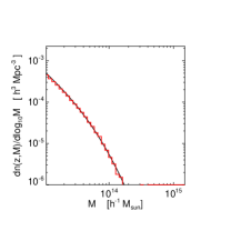
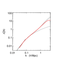
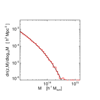
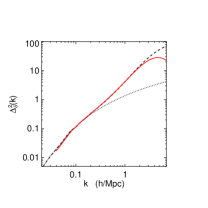
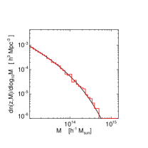
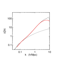
Figure 1.— Mass functions and 3-d power spectra for four tiles. From top to bottom the redshift of the tiles are $z_{\rm rear}=1.52,1.01,0.60,0.20$ (see Table 1 for simulation parameters). The left panels show the mass function (histogram) averaged over 38 different simulations of the same tile compared to the fitting formula (solid) of Jenkins et al. (2001). The right panels show the 3-d power spectra of the density field for each tile. Solid lines are the power spectra averaged over 38 simulations. Dashed curves show the nonlinear power spectra from the analytical fitting formulae of Smith et al. (2003) and dotted curves are the linear theory power spectra.

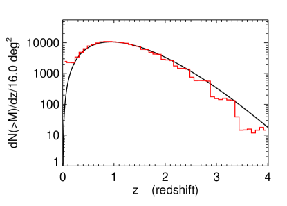
Figure 2.— Total number of clusters above $M=10^{13.5}\ h^{-1}{\rm\ M}_{\odot}$ in a $16\ {\rm deg}^{-2}$ patch of sky as a function of redshift. The histogram shows the redshift distribution averaged over 38 simulations. The solid line is the redshift distribution obtained from the fitting formula of Jenkins et al. (2001).

2.4. Mock Observations

The observables in weak lensing observations are the ellipticities of background source galaxies which have been distorted by the foreground matter distribution. Even for the ideal case of no instrumental noise, observations are limited by the intrinsic ellipticities of the sources and the finite number of Poisson distributed sources on the sky. Here we simulate this ideal case by drawing a number density $n$ of source galaxies from the source redshift distribution

$$p_{z}(z)=\frac{1}{2z_{0}^{3}}z^{2}e^{-z/z_{0}},$$ (5)

and placing them at random positions on our $4^{\circ}\times 4^{\circ}$ simulated field. This redshift distribution peaks at $2z_{0}$, has mean redshift $\langle z\rangle=3z_{0}$, and has been used in previous studies of cosmic shear (Wittman et al. 2000). A fraction $f_{z}$ of source galaxies will have photometric redshifts, where the errors are drawn from a Gaussian distribution with dispersion $\sigma_{z}=\delta_{z}(1+z)$ and added to the source redshifts. We take $n=40\ {\rm arcmin}^{-2}$, $z_{0}=0.50$ corresponding to a peak redshift of $z=1.0$, and $\delta_{z}=0.12$. Henceforth in this work we set $f_{z}=1$ and assume all source galaxies have photometric redshifts in order to determine the efficacy of our tomographic and adaptive matched filtering techniques for the best case.

The intrinsic ellipticities, $\epsilon_{\rm int}$, of the source galaxies are drawn from a Gaussian distribution with a single component rms dispersion $\gamma_{\rm rms}=0.165$ (Bernstein & Jarvis 2002). Note that there has been some confusion in the literature over the intrinsic ellipticity, and larger values have been employed in other studies. The value used here is achievable if the optimal weighting discussed in (Bernstein & Jarvis 2002) is applied to the sources for the asymptotic case of no instrumental noise (Gary Bernstein, private communication).

The simulations output convergence planes $\kappa(\hat{\bf n},z_{\rm rear})$ for $0\leq z_{\rm rear}\leq 4$ densely spaced in redshift as listed in Table 1, and the shear fields $\gamma(\hat{\bf n},z_{\rm rear})$ are obtained from the convergence via FFT using eqns. (3). A source galaxy at redshift $z$ is sheared by the nearest shear plane with $z_{\rm rear}<z$, via the weak lensing relation

$$\epsilon=\epsilon_{\rm int}+\gamma,$$ (6)

which is valid for $\kappa\ll 1$, $|\gamma|\ll 1$. The shear is interpolated from the grid onto the source galaxy position using bicubic spline interpolation. The end result is a mock catalog of source galaxy ellipticities with photometric redshifts, which we use to explore the statistics of clusters below.

In what follows we will want to compare mock observations with the noise properties described above with noiseless weak lensing observations in order to assess the intrinsic limitations of tomography and weak lensing searches for clusters. We define noiseless observations to be an infinite number of source galaxies with zero intrinsic ellipticity and photo-z error (i.e. $\gamma_{\rm rms}=0.0$ and $\delta_{z}=0$) drawn from the source redshift distribution in eqn. (5), and placed on the simulation grid rather than at random positions. Placing the source galaxies on the grid removes the Poisson clustering of the source galaxies, so that the angular resolution is then limited by the resolution of the simulation rather than shot noise. Because we cannot simulate an infinite number of sources, we draw 50 galaxies from eqn. (5) for each of the $512^{2}$ grid points, which we find is sufficient to converge to the limiting case of no noise. The left panel of Figure 3 shows a Kaiser-Squires reconstruction (Kaiser & Squires 1993) of the mean convergence field for noiseless data.

2.5. Matching Peaks with Clusters

Given a mock catalog of source galaxy ellipticities, we construct smooth maps by convolving the data with some filters. Candidate mass selected clusters will correspond to the peaks in these smoothed maps. We elaborate on the filtering techniques in the next section, but focus here on the details of matching the peaks in smoothed maps with clusters from the simulation tiles. We locate peaks in the maps using a simple algorithm whereby a peak is identified if it is higher than all of its neighboring pixels. While more complex algorithms exist to find peaks in pixelised data, because our maps have already been smoothed, searching for local maxima is sufficient. Given a list of peaks from the smoothed map and the cluster catalog constructed by applying FOF to the simulation tiles, we can correlate the peaks with the cluster catalog and locate all halos along the line of sight of a given peak. A peak in a map is considered a cluster detection if there is a cluster in the light cone within an aperture $\theta_{\rm match}=3^{\prime}$ centered on the peak. Although it might seem more appropriate to set this aperture size to the field of view of some ‘follow up’ instrument, $3^{\prime}$ is well matched to the angle subtended by the virial radius of a typical cluster at $z=0.4$, a typical redshift for a shear selected cluster. Further our interest here is in the primary object responsible for the lensing signal and not objects at larger angular separation that happen to be in the vicinity of the peak. In the event that there are multiple clusters within the aperture centered on the peak, we take the most massive cluster to be the ‘match’ to that peak. Depending on the method of follow up, the object most likely to be detected will be some function of mass and redshift, though we neglect this subtlety here. Finally, to avoid the problem of multiple peaks in the map corresponding to the same cluster, we keep only the highest peak in an aperture $\theta_{\rm iso}=1^{\prime}$ centered on each peak, so that less significant peaks near higher peaks are discarded.

3. Tomography and Matched Filtering

Previous studies (Reblinsky et al. 1999; White, van Waerbeke, & Mackey 2002; Padmanabhan, Seljak, & Pen 2003; Hamana, Takada, & Yoshida 2003), have neglected the extra information provided by photometric redshifts of source galaxies when searching for clusters in weak lensing data. Without redshift information, the source galaxy ellipticities provide a noisy measure of the mean shear

$${\bar{\gamma}}(\hat{\bf n})\equiv\int dzp_{z}(z)\gamma(\hat{\bf n},z),$$ (7)

which is the shear out to a given redshift averaged over the source redshift distribution $p_{z}(z)$. Knowledge of the source redshift enables one to measure the shear more accurately, and in this section we present a tomographic matched filtering scheme which fully incorporates this extra information.

The tomographic matched filtering (TMF) technique is similar in spirit to matched filtering algorithms used to find clusters in optical surveys (Postman et al. 1996; Kepner et al. 1999; White & Kochanek 2002; Kochanek et al. 2003) and is also qualitatively similar to the maximum likelihood techniques developed to study cluster mass profiles from weak lensing (Geiger & Schneider 1998; Schneider, King, & Erben 2000; King & Schneider 2001). In what follows we present a well-defined procedure for identifying clusters of galaxies in weak lensing surveys that makes optimal use of both the shape and photometric redshift information of the background source galaxies. It can be applied to weak lensing data for which only the overall source redshift distribution is known, for which photometric redshifts of the source galaxies are available, as well as combinations of the two scenarios (i.e. a fraction of galaxies with photometric redshifts and the rest with only shapes). Furthermore, we will see in §4 that a few source redshift bins perform nearly as well as full photometric redshift information, so simple color cuts and apparent magnitude priors can be used to extract the extra tomographic information.

The matched filter identifies clusters in weak lensing data by finding the peaks in a cluster likelihood map generated by convolving the source galaxy ellipticities with a filter that models the distortion caused by the foreground mass distribution. The peaks in the likelihood map will correspond to the locations where the match between the cluster model and the data is maximized, hence giving the two dimensional location of the cluster. In addition, the algorithm produces a tomographic estimate of the cluster redshift using the lensing signal, similar to the tomographic technique used by Wittman et al. (2001, 2003) and Taylor et al. (2004).

3.1. Formalism

The goal of the matched filter is to match the data to a model that describes the distortion of background galaxies by the foreground mass distribution, here a galaxy cluster. For the sake of generality, we parameterize the cluster lens by three quantities, a cluster redshift $z_{\rm d}$, an angular scale $\theta_{\rm s}$, and an amplitude $A$.

For a cluster at redshift $z_{\rm d}$ the convergence for a source galaxy at position $\vec{\theta}_{j}$ and redshift $z_{j}$ can be written

$$\kappa(\vec{\theta}_{j},z_{j})=Z(z_{j};z_{\rm d})\kappa_{\rm\infty}(\vec{\theta}_{j})$$ (8)

where

$$Z(z;z_{\rm d})\equiv\frac{D_{\rm ds}}{D_{\rm s}}H(z-z_{\rm d}),$$ (9)

and

$$\kappa_{\rm\infty}(\vec{\theta}_{j})=\frac{\Sigma(\vec{\theta}_{j})}{c^{2}D_{\rm d}/4\pi G}.$$ (10)

Here $\Sigma_{\rm crit}(z_{\rm d},z_{\rm s})=\frac{c^{2}}{4\pi G}\frac{D_{\rm s}}{D_{\rm d}D_{\rm ds}}$ is the critical density for lensing with $D_{\rm d}$, $D_{\rm ds}$, $D_{\rm s}$ the deflector, deflector-source, and source distances, respectively. The Heaviside step function accounts for the fact that sources in the foreground of the deflector are not lensed, and $\kappa_{\infty}$ is the convergence for a hypothetical source at infinite distance (see e.g. Seitz & Schneider 1997; King & Schneider 2001, for similar treatments). The same relationship holds for the shear, $\gamma(z)=Z(z;z_{\rm d})\gamma_{\infty}$. For a flat universe, eqn. (9) simplifies to

$$Z(z;z_{\rm d})=\max\left(1-\frac{D_{\rm d}}{D_{\rm z}},0\right).$$ (11)

In the weak lensing regime $\kappa\ll 1$, $|\gamma|\ll 1$, the observed complex ellipticity of a source galaxy is related to the shear field by eqn. (6). For a spherically symmetric mass distribution centered about the position $\vec{\theta_{0}}$, the shear will be entirely tangential

$$\gamma(\theta)=-\gamma^{T}(\vec{\theta};\vec{\theta_{0}})e^{2i\phi}$$ (12)

where $\phi$ is the azimuthal angle about the position $\vec{\theta_{0}}$. We employ the standard definition of the tangential shear

$$\gamma^{T}(\vec{\theta};\vec{\theta_{0}}) \equiv-[\gamma_{1}\cos(2\phi)+\gamma_{2}\sin(2\phi)]$$ (13)

$$=-\Re[\gamma(\vec{\theta}+\vec{\theta_{0}})e^{-2i\phi}]$$

and analogously for the tangential component of $\epsilon$, and hence the tangential ellipticity is related to the tangential shear by $\epsilon^{T}=\epsilon_{\rm int}^{T}+\gamma^{T}$. For our model cluster lens we take the mass distribution to be spherically symmetric, and henceforth work primarily with the tangential shear and tangential ellipticity.

For a cluster centered at position $\vec{\theta_{0}}$ with the parameter vector $(z_{\rm d},\theta_{s},A)$ the convergence can be written

$$\kappa_{\rm model}(\vec{\theta}_{j},z_{j};z_{\rm d},\theta_{\rm s},A) =\frac{\Sigma_{\rm model}}{\Sigma_{\rm crit}}$$

$$=Z(z_{j};z_{\rm d})A\ K(x_{j}),$$

where $x_{j}\equiv|\vec{\theta_{j}}-\vec{\theta_{0}}|/\theta_{\rm s}$, $K(x)$ is the cluster convergence profile in units of $\theta_{s}$, and the amplitude $A$ is given by

$$A\equiv\frac{\Sigma_{0}D_{\rm d}}{c^{2}/4\pi G},$$ (15)

where $\Sigma_{0}$ is the surface density normalization.

The tangential shear for this mass distribution is

$$\gamma_{\rm model}(\vec{\theta}_{j},z_{j};z_{\rm d},\theta_{s},A)=Z(z_{j};z_{\rm d})A\ G(x_{j})$$ (16)

where $G$ is related to $K$ by

$$G(x)=\frac{2}{x^{2}}\int_{0}^{x}K(y)ydy-K(x),$$ (17)

from the relation $\gamma=\bar{\kappa}-\kappa$. We omit the tangential superscript on $\gamma_{\rm model}$ and $\epsilon_{\rm model}$ for notational simplicity.

The probability of measuring a source galaxy with tangential ellipticity $\epsilon^{T}_{j}$ at position $\vec{\theta}_{j}$ with source redshift $z_{j}$, given the lens model in eqn. (16) is

$$P_{j}=\frac{1}{\sqrt{2\pi\sigma_{j}^{2}}}\exp\left[-\frac{1}{2}\frac{(\epsilon^{T}_{j}-\gamma_{\rm model})^{2}}{\sigma_{j}^{2}}\right]$$ (18)

The measurement error (assumed to be Gaussian) $\sigma_{j}^{2}$ in principle includes contributions from the intrinsic ellipticities of the source galaxies as well as an error term due to the photometric redshift error of the source galaxy at $z_{j}$, but in practice the former will dominate because of the the slow variation of the function $Z\left(z;z_{d}\right)$ in eqn. (11) with source redshift.

If the only knowledge of the source redshift comes from the aggregate source redshift distribution, one must work with the first moment of $Z(z)$ (Seitz & Schneider 1997; King & Schneider 2001), $\langle Z\rangle=\int dz\ p_{z}(z)Z(z;z_{\rm d})$ where $p_{z}$ is the source redshift distribution in eqn. (5). In this case, $\langle Z\rangle$ must be substituted for $Z$ in eqn. (16).

The likelihood of finding a cluster at position $\vec{\theta_{0}}$ with parameters $(z_{\rm d},\theta_{s},A)$, is the product over all the data of the individual probabilities

$$\mathcal{L}(\vec{\theta_{0}},z_{\rm d},\theta_{s},A)=\prod_{j}P_{j}$$ (19)

and the log likelihood is

$$\ln\mathcal{L}=-\frac{1}{2}\sum_{j}\ln(2\pi\sigma_{j}^{2})-\frac{1}{2}\sum_{j}\frac{(\epsilon^{T}_{j}-\gamma_{\rm model})^{2}}{\sigma_{j}^{2}}.$$ (20)

Expanding the expression in eqn. (20) and dropping terms that do not depend on the parameter vector gives

$$\ln\mathcal{L}=\frac{1}{2}\sum_{j}\frac{(2\epsilon^{T}_{j}\gamma_{\rm model}-\gamma^{2}_{\rm model})}{\sigma_{j}^{2}}.$$ (21)

This expression has a linear dependence on $A$, which can be exploited to lower the dimensionality of the fit. Setting the derivative of eqn. (21) with respect to $A$ to zero gives

$$A(z_{\rm d},\theta_{s})=\frac{\sum_{j}\frac{1}{\sigma_{j}^{2}}\epsilon^{T}_{j}ZG}{2\sum_{j}\frac{1}{\sigma_{j}^{2}}Z^{2}G^{2}}$$ (22)

Substituting this back into eqn. (21) finally gives

$$\ln\mathcal{L}(\vec{\theta_{0}},z_{\rm d},\theta_{s})=\frac{1}{2}\sum_{j}\frac{\epsilon^{T}_{j}\gamma_{\rm model}}{\sigma_{j}^{2}}.$$ (23)

Thus, the log likelihood is a convolution of the data with a ‘matched filter’, with each source galaxy inverse weighted by its respective error. The technique is ‘adaptive’ in that it searches for parameters $(z_{\rm d},\theta_{s},A)$ that maximizes the contrast between the cluster and the background noise, making full use of the additional information provided by photometric redshifts of source galaxies, which is reflected in the redshift ‘weights’ used in eqn. (16).

Ideally, one would perform the convolution in eqn. (23) with the fast algorithms introduced and applied to weak lensing by Padmanabhan, Seljak, & Pen (2003), which do not require spatial binning. Here for simplicity, we opt to use FFT methods. Doing the convolutions with FFT’s requires binning the source galaxies both spatially and in redshift. In the event that the scale of the matched filter, $\theta_{\rm s}$, is kept fixed when maximizing the likelihood, then the convolution in eqn. (23) can be done with a single FFT for each redshift bin, as we see below.

For the spatial binning we follow Seitz & Schneider (1996) and write the complex ellipticity at any gridpoint $k$ as

$$\epsilon(\vec{\theta_{k}})=\frac{\sum_{j}W_{j}\epsilon_{j}}{\sum_{j}W_{j}}$$ (24)

with

$$W_{j}=\exp\left(-\frac{|\vec{\theta_{j}}-\vec{\theta_{k}}|^{2}}{2\Delta\theta^{2}}\right)$$ (25)

where $\Delta\theta$ is a smoothing length.

In choosing the source galaxy redshift bins, we take $p_{z}(z)$ into account and require each bin to have an equal fraction of the probability. Because the function $Z\left(z;z_{d}\right)$ in eqn. (11) varies slowly with redshift for $z>z_{\rm d}$, this binning can be relatively coarse. We consider two different binnings: a coarse binnning with only 3 bins, as might be achieved by using as little as two colors and an apparent magnitude prior, and a finer set of 5 bins which would require multi color data. We don’t simulate the effects of errors in assigning galaxies to their respective bins. The spacing of the bins is chosen to contain equal probability as given by the source redshift distribution in eqn. (5). The redshift ranges of the bins and the central redshift are listed in Table 2. We will henceforth refer to the TMF with three coarse bins as the TMF3 and that with five finer bins as the TMF5.

Table 2Source Redshift Binning

Type	$z_{\rm low}$	–	$z_{\rm high}$	$z_{\rm center}$
	0	–	1.02	0.70
Coarse	1.02	–	1.72	1.34
	1.72	–	$\infty$	2.28
	0	–	0.77	0.55
	0.77	–	1.14	0.96
Fine	1.14	–	1.55	1.34
	1.55	–	2.14	1.81
	2.14	–	$\infty$	2.66

NOTES.— Source redshift binnings used in this paper. The “Coarse” binning uses three redshift bins, while the “Fine” binning uses five. Bins are chosen to contain equal probability from the source redshift distribution in eqn. 5. Lower, upper, and central redshift are denoted by $z_{\rm low}$, $z_{\rm high}$, and $z_{\rm center}$, respectively.

Combining eqns. (22) and (24) with the log likelihood in eqn. (23) gives

$$\ln\mathcal{L}(\vec{\theta_{0}},z_{d},\theta_{s})=\frac{1}{2\sigma^{2}}\frac{\left(\sum_{i}^{n_{z}+1}Z(z_{i};z_{d})\sum_{k}^{n_{g}}\epsilon^{T}_{ik}G(x_{k})\right)^{2}}{\sum_{i}^{n_{z}+1}Z^{2}(z_{i};z_{d})\sum_{k}^{n_{g}}G^{2}(x_{k})}$$ (26)

Here $\epsilon^{T}_{ik}$ is the tangential ellipticity about $\vec{\theta_{0}}$ at gridpoint $k$ for source galaxies in the $i$th redshift bin. The number of grid points and source redshift bins are denoted by $n_{g}$ and $n_{z}$ respectively. The sum over $i$ extends to $n_{z}+1$ to indicate that the last bin will be those galaxies that do not have photometric redshifts, for which the mean value of $\langle Z\rangle(z_{d})$ must be used. For simplicity we have taken all the ellipticity errors to be the same, $\sigma\equiv\sigma^{2}_{j}$. This can be easily generalized to the general case of different errors for each source galaxy, which would amount to modifying eqn. (24) to take the different errors into account. Note that the sum over $k$ in the numerator of this last expression for the likelihood is just a convolution of the tangential shear with the ‘matched filter’ $G(x_{k})$ which can be done using an FFT.

If we define

$$M_{i}(\vec{\theta_{0}})\equiv\frac{\sum_{k}^{n_{g}}\epsilon^{T}_{ik}G(x_{k})}{\left[\sum_{k}^{n_{g}}G^{2}(x_{k})\right]^{1/2}},$$ (27)

then the likelihood can finally be written

$$\ln\mathcal{L}(\vec{\theta_{0}},z_{d},\theta_{s})=\frac{1}{2\sigma^{2}}\frac{\left(\sum_{i}^{n_{z}+1}Z(z_{i};z_{d})M_{i}(\vec{\theta_{0}})\right)^{2}}{\sum_{i}^{n_{z}+1}Z^{2}(z_{i};z_{d})},$$ (28)

where $M_{i}(\vec{\theta_{0}})$ is the convolution of the ellipticity of the source galaxies in the $i$th redshift bin with the normalized kernel $G(x_{k})/[\sum_{k}G^{2}(x_{k})]^{1/2}$. If there is no photometric redshift information, $n_{z}=0$, the redshift weight factors of $\langle Z\rangle^{2}(z_{d})$ in the numerator and denominator of eqn. (28) will cancel, and the log likelihood just reduces to the square of a single map $M(\vec{\theta_{0}})$, which is a convolution of the tangential shear with the normalized kernel. It is only this limiting case which has previously been considered by studies that neglect photometric redshift information (Reblinsky et al. 1999; White, van Waerbeke, & Mackey 2002; Padmanabhan, Seljak, & Pen 2003; Hamana, Takada, & Yoshida 2003).

The expression for the likelihood in eqn. (28) can be maximized at each point on the sky, allowing one to create a cluster likelihood map. Clusters will be located at the peaks in this map and the maximum likelihood $z_{d}$ will be the tomographic estimate for the lens redshift.

An example of a likelihood map constructed from binned source galaxies is depicted in Figure 3. The left panel shows a Kaiser-Squires reconstruction of the mean convergence field (recall eqn. 7) for the case of no noise. The right panel shows the cluster likelihood map constructed by applying the TMF to mock data which includes noise. Three coarse source redshift bins have been used to make this map (TMF3). For the function $G(x)$ we have used the ‘optimal filter’ determined in §4 below (eqn. (34) with a scale angle,$\theta_{s}=0.50^{\prime}$, and gaussian truncation radius, $\theta_{\rm out}=5.5^{\prime}$), which maximizes the number of clusters detected. This filter approximates a projected Navarro-Frenk-White Navarro, Frenk, & White (1997) (NFW) profile, but is truncated with a Gaussian to prevent the likelihood sum from being diluted by distant uncorrelated source galaxies. Peaks in the likelihood map are candidate shear selected clusters and four of the more significant peaks in this map are circled and labeled a-d.

The probability distributions of the tomographic redshift for each of these four peaks is shown in Figure 4. To create the likelihood map in Figure 3 the source galaxies were binned spatially and in redshift as in eqn. (26); however, to compute the probability distributions shown in Figures 4, the convolution in eqn. (23) is performed exactly in real space with no binning. The mass and redshift of the cluster(s) responsible for the peaks are labeled, and the vertical dashed lines indicate the true lens redshift(s).

Although we will consider the accuracy of the tomographic redshifts in detail in §5, the examples in Figure 4 illustrate some qualitative features of the tomographic technique which we elaborate on them briefly.

Peak a corresponds to a fairly massive cluster at $z=0.29$ and the tomography performs well, giving a tomographic redshift of $z=0.26$. For the higher redshift cluster coincident with peak b, at $z=0.70$, the tomography gives $z_{d}=0.95$, which is incorrect, but the tomography succeeds to indicate that the deflector is at high redshift, which is still helpful as the source galaxies can be weighted for a high redshift deflector, increasing the contrast between the cluster and the noise.

Projections of several halos at different redshifts are quite common, which is illustrated by peak c which is a projection of a $2\times 10^{14}\ h^{-1}{\rm\ M}_{\odot}$ cluster at $z=0.27$ and two large group size halos of $5\times 10^{13}\ h^{-1}{\rm\ M}_{\odot}$ at $z=0.53$ and $z=1.06$, respectively. Notice in Figure 4, that the tomography gives a deflector probability distribution with two likelihood maxima at redshifts corresponding to the two redshifts of the lower redshift halos. The fact that the peaks in the probability line up with the deflector redshifts is somewhat of a coincidence, since we are fitting a model to the shear with only a single deflector.

Finally, as we will elaborate on further in the next section, mass selected cluster samples are plagued by projection effects due to large scale structure and small halos along the line of sight. Although the peak labeled d is the highest peak in the likelihood map, there is no corresponding halo in the light cone above $10^{13.5}\ h^{-1}{\rm\ M}_{\odot}$ within an aperture of radius $3^{\prime}$ (which is our peak-halo matching criteria). However, there is no indication that this peak is a projection from the tomography, which gives a probability distribution similar to the others indicating the tomographic redshift is $z_{d}=0.36$. It is perhaps not surprising that $z_{d}\approx 0.4$, when one considers that the lensing efficiency peaks at this redshift, and large scale structure along the line of sight weighted by this lensing kernel is likely to yield a tomographic redshift at its peak.

Although the tomographic redshift probability distribution radially resolved two projected clusters for peak c, it led us to believe that peak d was a shear selected cluster just like any other, at $z_{d}=0.36$, when in reality it was a projection of large scale structure. A detailed investigation of the degree to which cluster tomography can distinguish projections from real clusters is beyond the scope of this work. If it were possible to make a such a distinction based on the tomography, one could imagine flagging certain these peaks, so that a shear selected cluster sample could be cleaned of such projections, which will complicate attempts to determine cosmological parameters from the redshift distribution of shear selected clusters. Of course, the projection hypothesis can also be tested by searching for overdensities of early type galaxies (i.e. cluster galaxies associated with the lenses) as a function of photometric redshift

(Dahle et al. 2003; Schirmer et al. 2003, 2004; Taylor et al. 2004).

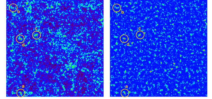
Figure 3.— Left panel: Kaiser-Squires reconstruction of the mean convergence field, ${\bar{\kappa}}$, for noiseless mock data. Right panel: Cluster likelihood map constructed with the TMF applied to noisy data. Source galaxies were binned into three coarse redshift bins (TMF3). Cluster statistics and the tomographic redshift probability distributions for the four clusters labeled a-d are shown in Figure 4.

.

Figure 4.— Cluster statistics and the tomographic redshift probability distributions for the four clusters labeled a-d in Figure 3. The mass, $M_{14}=M/10^{14}\ h^{-1}{\rm\ M}_{\odot}$, and redshift, $z$, of the cluster(s) responsible for each peak are labeled. Vertical dashed lines indicate the true redshifts of the halos along the line of sight. The location of the peak of the probability is the tomographic redshift, $z_{d}$, which is also labelled.

4. The Optimal Filter

4.1. Discussion of Filter Functions

In this section we will consider several filter functions $G(x)$ to convolve the tangential shear data with for the TMF introduced in §3. But first, a few general remarks about searching for clusters in weak lensing data are in order.

Like the $\zeta$ statistics (Fahlman, Kaiser, Squires, & Woods 1994) and the aperture mass measures $M_{\rm ap}$ (Schneider 1996), The TMF has the virtue that it operates directly on the shear, which is the observable quantity in weak lensing observations. Some studies of shear selected cluster detection search for clusters by first performing a Kaiser-Squires density reconstruction, and then smoothing the reconstructed convergence field with a filter and searching for peaks (Reblinsky et al. 1999; White, van Waerbeke, & Mackey 2002; Hamana, Takada, & Yoshida 2003). However, working directly with the shear is crucial, when one recalls that the surface mass density at any point depends on the galaxy ellipticities at all distances (see e.g., Bartelmann & Schneider 2001). The kernel that the ellipticity data is convolved with in a density reconstruction is not local, decaying as $\theta^{-2}$. Because of edge effects from the field boundaries and all the masked bright stars, diffraction spikes, and bleed trails (see Figure 14 of Van Waerbeke & Mellier (2003) for a nice example), the non-local Kaiser-Squires reconstruction will propagate ringing from this ‘window function’ into other regions of the mass map, significantly amplifying noise. It should thus be avoided for the purposes of finding clusters.

Besides avoiding the deleterious effect of the noisy window function or mask, convolving the shear with a compact kernel seems sensible because clusters of galaxies have characteristic size on the sky. However, weak lensing statistics using small apertures are complicated by the non-local relationship between shear and mass. Any filter convolved with the shear within some aperture will have fluctuations imprinted on it from scales outside that aperture. The simplest case is the mass sheet degeneracy, whereby the convergence field reconstructed from a source galaxies in a finite field can only be determined up to an additive constant or sheet of mass (Bartelmann & Schneider 2001). While the mass sheet can be intuitively identified with fluctuations in the $\ell\sim 0$ mode, all large scale structure fluctuations on scales larger than the aperture $\theta$, $\ell\lesssim 1/\theta$, result in a variance of any statistic we apply to the shear over a finite aperture. Hoekstra (2001, 2003) and Dodelson (2003) have studied the effect of the variance due to large scale structure on measurements of cluster masses and density profiles. For the purposes of identifying clusters, variance in our aperture statistic will increase the number of false detections, lowering the efficiency of cluster finding.

The aperture mass measures (Schneider 1996; Schneider et al. 1998) constitute a class of filters which mitigate the aforementioned problem. Convolution of the $\kappa$ map with a kernel $U$ can be shown to be equivalent to convolving the tangential shear map with a related kernel $Q$, provided that the kernel $U$ is compensated

$$\int_{0}^{1}dxxU(x)=0.$$ (29)

In this work we consider the most widely used pair of kernels $U$ and $Q$ which are

$$U(x) = \frac{9}{\pi\vartheta^{2}}(1-x^{2})\left(\frac{1}{3}-x^{2}\right)$$

$$Q(x) = \frac{6}{\pi\vartheta^{2}}x^{2}\left(1-x^{2}\right),$$ (30)

where $\vartheta$ is the size of the aperture and $x=\theta/\vartheta$.

The aperture mass has the appealing property that it provides a lower limit on the mass contained within the aperture $\theta$, because of its equivalence to a convolution of $\kappa$. Furthermore, it is relatively unaffected by modes larger than the filter scale. As shown by Schneider et al. (1998), its variance can be written

$$\langle M^{2}_{\rm ap}\rangle=\int d\ln\ell~{}\Delta_{\kappa}^{2}(\ell)F(\ell\vartheta)$$ (31)

where $F(\ell\vartheta)$ is a notch filter which peaks at $\ell\sim\vartheta$ and suppresses fluctuations from scales smaller and larger. The fact that the aperture mass is insensitive to the mass sheet degeneracy is manifest by the fact that $F(\ell=0)=0$. Because modes larger and smaller than the aperture scale (matched to the size of a cluster) don’t cause fluctuations in the aperture mass, we might expect this filter to more efficiently locate clusters in weak lensing data. We return to this point below.

A potential problem with using the aperture mass is that because it is compensated (eqn. 29) it does not provide a very good fit to the tangential shear profile of a galaxy cluster. Hence, we don’t expect it to work as well with the tomographic technique introduced in the previous section.

Padmanabhan, Seljak, & Pen (2003) advocate using a matched filter with convergence profile

$$K_{\rm NFW}(x)=\frac{1}{(1+x)^{2}}.,$$ (32)

where $x=\theta/\theta_{s}$, for several different values of the scale angle $\theta_{\rm s}$. This profile approximates an NFW density profile (Navarro, Frenk, & White 1997) in projection, and has been used in studies of optical clusters (White & Kochanek 2002; White et al. 2002). The tangential shear corresponding to this convergence profile is

$$G_{\rm NFW}(x)=\frac{2\ln(1+x)}{x^{2}}-\frac{2}{x(1+x)}-\frac{1}{(1+x)^{2}},$$ (33)

where we have applied eqn. (17).

The soft core in this profile is a desirable feature, since convolving shear data with a divergent profile gives a large weight to a single noisy galaxy resulting in an ultraviolet divergence, as is well known in the literature on weak lensing mass reconstructions (see Kaiser & Squires 1993). However, these NFW convergence and shear profiles decay asymptotically as a power law $\sim\theta^{-2}$, and are not compact. As we will see, this has a deleterious effect on the number of clusters detected and on the efficiency of the cluster search, because of a dramatic increase in confusion from large scale structure.

The foregoing discussion motivates the truncated projected NFW profile

$$G(x)=G_{\rm NFW}(x)\exp\left(-\frac{\theta^{2}}{2\theta_{\rm out}^{2}}\right),$$ (34)

where we have truncated the filter in eqn. (33) by multiplying with a Gaussian of truncation angle $\theta_{\rm out}$.

Note that the model shear profile in eqn. (34) now has two free scale parameters $\theta_{\rm s}$ and $\theta_{\rm out}$, whose values we must determine. In principle, we could leave them as parameters, and maximize the likelihood in eqn. (23) with respect to redshift and both angular scale factors. Tests on the simulations indicate that for fixed $\theta_{\rm out}$, maximizing the likelihood with respect to scale angle $\theta_{\rm s}$ and $z_{d}$ performs slightly worse than the case where $\theta_{\rm s}$ is fixed and the likelihood is maximized only with respect to $z_{\rm d}$. Furthermore, varying the scale angle $\theta_{s}$ would require performing a whole sequence of convolutions with different size filters, which is more expensive computationally. For these reasons we choose to fix $\theta_{\rm s}=0.50^{\prime}$, which is roughly matched to both the pixel size in our simulated maps and the angle $\theta_{\rm s}$ subtended by the scale radius $r_{\rm s}$ of a $10^{14}\ h^{-1}{\rm\ M}_{\odot}$ NFW cluster at $z\simeq 0.4$. Varying this scale angle from $\theta_{\rm s}=0.10-0.70$ produces negligible changes in our results.

Maximizing the likelihood with respect to the truncation angle $\theta_{\rm out}$ also performs poorly, because of a tendency to overfit noise and large scale structure on scales much larger than the size of a cluster. Also, the likelihood for small and large $\theta_{\rm out}$ will be over a different number of source galaxies and hence degrees of freedom. Thus their distributions will have different means and variances, complicating a comparison of the resulting likelihoods. For these reasons, we take the truncation radius $\theta_{\rm out}$ to be a ‘prior’ that we vary by hand, until the number of clusters detected for a given noise model is maximized.

In addition to the aperture mass (eqn. (4.1)), the projected NFW profile (eqn. (33)), and the truncated NFW (eqn. 34)), we also try simply convolving the tangential shear with a Gaussian filter of size $\theta_{\rm out}$.

In general, the degree of smoothing required to detect clusters from weak lensing data will depend on the level of noise for the particular set of observations, as higher noise will require more smoothing. Here we focus on the noise model described in §2. Adapting a filtering scheme to different levels of noise will amount to varying the overall extent of the filter.

4.2. Comparison of Filters

Searching for shear selected clusters entails convolving the ellipticity data with a filter and searching for peaks in a map. In general some signal to noise ratio threshold, $\nu$, will be chosen such that peaks above this threshold are considered candidate clusters and peaks below it are discarded. Given a threshold $\nu$, a fraction of all peaks larger than $\nu$ will be identified as galaxy clusters and the remainder will correspond to false detections.

We define the efficiency as a function of this threshold as

$$e(\nu)\equiv\frac{n_{\rm clusters}(>\nu)}{n_{\rm peaks}(>\nu)}.$$ (35)

It is clear that raising the threshold $\nu$, will increase the efficiency, but at the expense of fewer detections $n_{\rm clusters}(>\nu)$, since there will be fewer total peaks greater than $\nu$. Rather than fix $\nu$ at say 5$\sigma$, where $\sigma$ represents the variance of the noise, we consider the number of clusters detected as this threshold is varied. There are several reasons why one may wish to work at low thresholds and hence low efficiency, but we defer a discussion of this point to §5. Note that the definition in eqn. (35) allows us to assign an efficiency to any peak $\nu$ in our maps, and we may speak of an efficiency cutoff of say 75%, where it is understood that the we keep all clusters above the threshold $\nu_{75}$ where $e(\nu_{75})=75\%$.

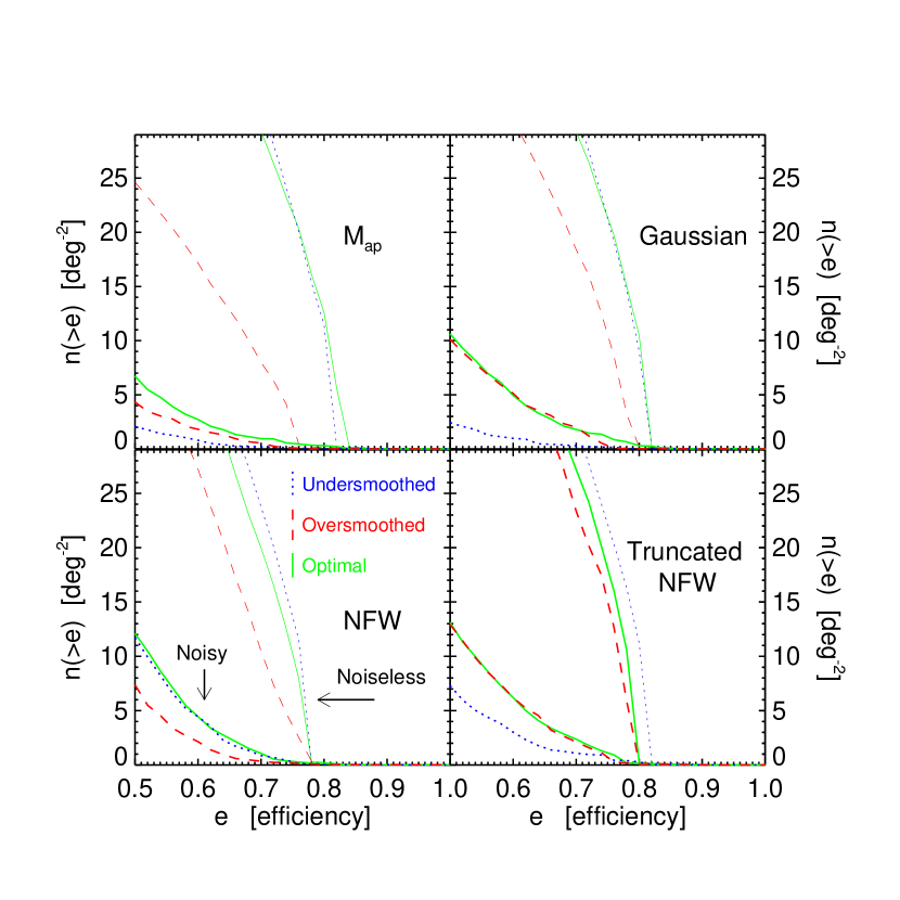
Figure 5.— Number density of clusters versus efficiency for four filters. Dotted (blue) curves are undersmoothed, dashed (red) curves are over smoothed, and solid (black) curves indicate the filter size that performs best. The inner set of curves are noisy mock data and the thin outer curves are for noiseless data. A summary of information on the filters and aperture scales used in this figure is given in Table 3.

In Figure 5 we plot the number of clusters detected per square degree versus efficiency for the filters discussed above. All the aforementioned filters have an angular scale parameter, and will yield more or less clusters at a given efficiency as this scale is varied. For the aperture mass this scale is the size of the aperture $\vartheta$. The only scale in the NFW profile in eqn. (32) is the scale angle $\theta_{\rm s}$. For the truncated NFW and the Gaussian, the scale parameter is the Gaussian cutoff angle $\theta_{\rm out}$. For each filter we plot two sets of curves corresponding to noisy and noiseless mock weak lensing data, with the outermost thin curves corresponding to the noiseless case.

As the amount of smoothing is increased there is a tradeoff between averaging over more source galaxies, and hence increasing the signal to noise on the one hand, but increasing the level of confusion from cosmic structure and merging distinct clusters together into one another. For a given amount of noise, the optimal scale for a filter corresponds to the curve furthest to the right in Figure 5, which maximizes the number of clusters detected at each efficiency. The dotted (blue) and dashed (red) curves correspond to under and over smoothing, respectively, and the solid (green) curves correspond to the ‘optimal’ scale for the noisy data. Table 3 summarizes the information for the filters discussed in this section and plotted in Figure 5. The optimal smoothing scale is printed in bold.

Table 3Filters used in Figure 5

Filter	Profile Eqn	Scale Angle	Angles
NFW	(33)	$\theta_{\rm s}$	0.01,0.1,1.0
$M_{\rm ap}$	(4.1)	$\vartheta$	2.0,3.0, 5.0
Gaussian	—	$\theta_{\rm out}$	1.5,2.0, 4.5
Truncated NFW	(34)	$\theta_{\rm out}$	2.0, 5.5, 10.0

NOTES.— Parameters for the four filters functions $G(x)$ (see eqn. 16) used in Figure 5. The table lists the defining equation of the profile, the angular scale parameter varied to set the level of smoothing, and the three angles used in the figure. The three angles correspond to undersmoothing (dotted curves in Figure 16), the optimal smoothing, (solid curves), and oversmoothing (dashed curves), respectively. The optimal smoothing is listed in bold and all angles are in arcminutes. t

Figure 6.— Number density of clusters versus efficiency for four filters using varying degrees of photometric redshift information. Dotted (blue) curves use no photometric redshift information, dashed (red) are for sources binned into five fine photometric redshift bins (TMF5), and solid (green) curves are for the sources binned into three coarse redshift bins (TMF3). The inner set of curves are noisy mock data and the thin outer curves are for noiseless data. The TMF exploits the information provided by source photometric redshifts to increase the number of clusters detected at all efficiencies, even for crude redshift bins. A comparison of the performance of these filters is presented in Table 4.

Figure 7.— Comparison of the four filter functions with and without tomography. The left panel uses no photometric redshift information, whereas the right panel uses tomography with source galaxies binned into three coarse redshift bins (TMF3). The optimal filtering scale is used for each filter (see Table 3). The inner set of curves are for noisy data and the thin outer curves are noiseless. The dot-dashed (magenta) curve is for the NFW profile, the dashed (red) curve is the aperture mass, the dotted (blue) curve is the Gaussian, and the solid (green) curve is the truncated NFW. The amount by which tomography enhances the performance of each filter is listed in Table 4.

The benefit of using photometric redshift information is illustrated in Figure 6, where we smoothed with the optimal filter scale for each filter as determined from Figure 5 and listed in Table 3, but varied the amount of photometric redshift information used. The dotted (blue) curves ignore photo-z information, the solid (green) curves correspond to the TMF with the three coarse photometric redshift bins (TMF3), and the dashed (red) curves correspond to the TMF with the five finer (TMF5) photometric redshift bins (see Table 2). Both TMF’s detect significantly more clusters for each filter at high and low efficiencies.

We quantify the increase in clusters detected with the TMF in Table 4, where we list the number of clusters per square degree with and without tomography. We compare all four filters at a high efficiency cutoff of $e=75\%$ and a lower cutoff of $e=60\%$. To get an idea of the signal to noise ratios corresponding to the efficiency thresholds, we also list the signal to noise ratio at the efficiency cutoff, $\nu_{75}$ and $\nu_{60}$, of the filtered maps which did not use tomography. The noise in the maps was computed by calculating the variance of smoothed maps of unlensed source galaxies which had the same positions and intrinsic ellipticities as the lensed sources. An efficiency of $e\geq 75\%$ corresponds to peaks with a signal to noise ratio $\nu\gtrsim 4.5$, whereas $e\geq 60\%$ corresponds to signal to noise cutoff of $\nu\gtrsim 3.5$. The TMF increases the number of $\nu\gtrsim 4.5$ peaks by up to $76\%$. For lower thresholds, the increases in the number of clusters detected is less substantial ($\sim 30\%$), because the tomography is less effective at determining the redshift of the cluster for lower signal to noise detections. The TMF increases the number of clusters detected for all filters; however, the gains are more substantial for the truncated NFW profile which best approximates the tangential shear profile of clusters.

Besides increasing the total number of clusters detected, the TMF substantially increases the dynamic range of the resulting cluster sample. The redshift and mass number count distributions detected by the truncated NFW profile for an efficiency cutoff of $e\geq 75\%$ are shown in Figure 8. The solid histogram is for the TMF3 whereas the dotted (blue) line does not use photometric redshifts. At low redshifts and high mass, the number of clusters detected are nearly the same, however the TMF detects many more high redshift clusters and it extends the mass sensitivity down to the scale of large groups.

As is evident from Figures 6, 8, and Table 4, dividing source galaxies into three coarse redshift bins is sufficient to reap the benefits of tomographic information and increase the number of clusters detected. Such a coarse redshift division can be achieved with as few as two colors and an apparent magnitude prior, so that the TMF can be used with deep imaging data in as few as three pass bands.

A comparison of the four filters we consider is presented in Figure 7. The filters shown are the optimal aperture mass ($\vartheta=3.0^{\prime}$) , Gaussian ($\theta_{\rm out}=2.0^{\prime}$), NFW ($\theta_{\rm s}=0.1^{\prime}$), and truncated NFW ($\theta_{\rm out}=5.5^{\prime}$). The left panel doesn’t use tomography and the right panel is for the TMF3. The thin outermost set of curves are for noiseless data.

For noisy data, the truncated NFW is most effective at finding clusters for efficiency cuts between $60-75\%$, corresponding to detection significance of $\nu=3.5-4.5$, detecting $\sim 20-30\%$ more clusters, especially if tomography is used. The non-truncated NFW filter performs significantly worse than the others, even at very high signal to noise ratios, because it is not compact enough, dropping off as $\theta^{-2}$.

At the highest efficiencies $e\gtrsim 0.8$ corresponding to peaks with $\nu_{80}\gtrsim 6$, the aperture mass detects more clusters than the other filters. For these highest peaks, the aperture mass is less affected by large scale structure and noise, and does the best job of sorting out projection effects. Whereas the truncated NFW ranks peaks by some combination of mass and also goodness of fit to the NFW profile, by definition, the aperture mass ranks peaks by mass, since it provides a lower limit on the mass enclosed within the aperture. Further, this result is not unexpected in light of our discussion of the variance of the aperture mass (eqn. 31) in §4.1. Notch filtering of the shear field results in a smaller variance from both noise and large scale structure, which for the most massive clusters $\sim 10^{15}\ h^{-1}{\rm\ M}_{\odot}$ clusters, increases the efficiency of the cluster search.

A conspicuous feature of Figures 5, 6, and 7, is that even for the unachievable case of no intrinsic ellipticity or Poisson noise, the maximum intrinsic efficiency of weak lensing cluster searches is only $\sim 85\%$. Thus $\sim 15\%$ of even the most significant peaks detected in noiseless weak lensing maps do not have a collapsed halo with $M>10^{13.5}\ h^{-1}{\rm\ M}_{\odot}$ within 3 arcmintues (which is our peak halo matching criteria). This intrinsic inefficiency is due to projection effects and to confusion from cosmic structures, and has been noted by previous studies (Metzler, White, & Loken 2001; White, van Waerbeke, & Mackey 2002; Padmanabhan, Seljak, & Pen 2003; Hamana, Takada, & Yoshida 2003). This fact sheds light on the purported detections of ‘dark clumps’ reported recently by several groups (Fischer 1999; Erben et al. 2000; Umetsu & Futamase 2000; Miralles et al. 2002; Dahle et al. 2003). These objects could be entirely consistent with the $\sim 15\%$ false detections, though a definitive conclusion will have to wait for future wide field weak lensing surveys. Because of the intrinsic inefficiency that we find here, only statistical statements can be made about a population of dark clusters.

Table 4Filter Comparison

Filter	$\nu_{60}$	$n(>60\%)$	$n_{\rm TMF3}(>60\%)$	$n_{\rm TMF5}(>60\%)$	% increase	$\nu_{75}$	$n(>75\%)$	$n_{\rm TMF3}(>75\%)$	$n_{\rm TMF5}(>75\%)$	% increase
NFW	4.1	4.45	5.34	6.27	41	6.3	0.28	0.34	0.29	19
$M_{\rm ap}$	3.5	2.72	3.33	3.38	25	4.5	0.48	0.63	0.51	33
Gaussian	3.4	4.94	6.38	6.54	32	4.4	1.10	1.47	1.28	34
Truncated NFW	3.4	6.20	7.53	7.70	24	4.9	0.99	1.75	1.45	76

NOTES.— Comparison of filters with and without tomography. The number of clusters detected per square degree without tomography, with coarse redshift tomography (TMF3), and fine redshift tomography (TMF5), are denoted by $n$, $n_{\rm TMF3}$, and $n_{\rm TMF5}$. Two efficiency thresholds are compared, $60\%$ and $75\%$, and the $S/N$ ratio threshold (computed from the maps without tomography) corresponding to each efficiency cut, $\nu_{60}$ and $\nu{75}$, are listed. The column labeled “% increase” shows the improvement when tomography is used of either the TMF3 or TMF5, whichever is greater.

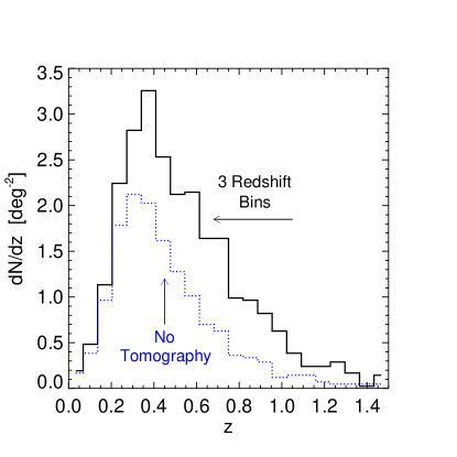
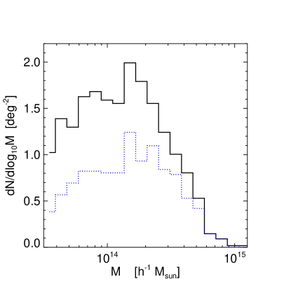
Figure 8.— Redshift (left) and mass (right) number count distributions of clusters detected by the truncated NFW with and without tomography. Dotted (blue) histograms do not use photometric redshift information while solid (black) histograms are for the source galaxies binned into three coarse redshift bins (TMF3). The cluster samples used to construct these histograms used an efficiency cutoff of $e\geq 75\%$ corresponding to a $S/N\gtrsim 4.5$. Even with just three coarse redshift bins, the TMF increases the number of clusters detected by $76\%$ (see Table 4). Tomography increases the dynamic range of weak lensing searches for clusters, detecting more high redshift clusters and extending the mass sensitivity down to the scale of large groups.

5. Completeness of Shear Selected Samples

In this section we discuss the completeness of shear selected cluster samples detected by the filter which performed best in the previous section. Specifically, we consider the truncated NFW filter with $\theta_{\rm out}=5.5^{\prime}$ without photometric redshift information and with source galaxies binned into three coarse redshift bins (TMF3). The left panel of Figure 9 shows the completeness as a function of redshift for all clusters with $M>10^{14.3}~{}h^{-1}{\rm\ M}_{\odot}$. The right panel shows completeness as a function of cluster mass for clusters in the redshift range $0.2<z<0.8$. Thick lines are for an efficiency cutoff of $e\geq 60\%$ ($S/N\gtrsim 3.5$) whereas thin lines are for $e\geq 75\%$ $S/N\gtrsim 4.5$. For the lower efficiency cut of $e\geq 60\%$, the completeness is $\gtrsim 50\%$ only for the most massive clusters $M\gtrsim 10^{14.3}$ which are near the peak of the lensing efficiency at $z\sim 0.3$. Limiting the cluster search to the higher efficiency threshold $e\geq 75\%$ further reduces the completeness by $\sim 40\%$. As a function of cluster mass the completeness only approaches unity for the most massive clusters $M\sim 10^{15}~{}h^{-1}{\rm\ M}_{\odot}$, where we begin to suffer from small number statistics.

Previous studies of shear selected clusters carried out by several groups (White, van Waerbeke, & Mackey 2002; Padmanabhan, Seljak, & Pen 2003; Hamana, Takada, & Yoshida 2003) come to a similar conclusion. Namely, that shear selected cluster samples suffer from severe incompleteness except at the highest masses. Although our results are broadly consistent with these studies, a direct comparison is difficult because the noise levels, source redshift distributions, aperture to match peaks to clusters, and filtering techniques employed are all different. In particular White, van Waerbeke, & Mackey (2002) and Hamana, Takada, & Yoshida (2003) use a single source redshift plane which implies the lensing efficiency will be a narrower function of redshift than that given by the source redshift distributions considered here and in Padmanabhan, Seljak, & Pen (2003). A source redshift distribution results in lower completeness than a single source plane (Padmanabhan, Seljak, & Pen 2003) because the broader lensing kernel increases noise from projections of large scale struture.

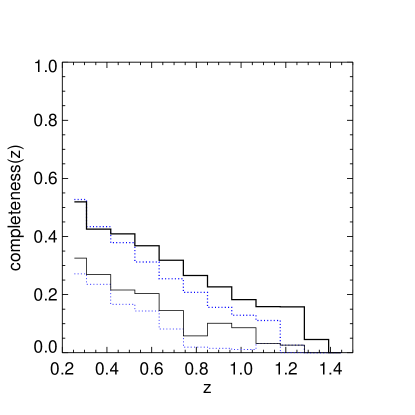
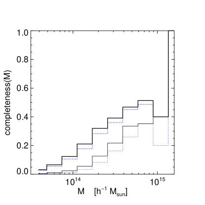
Figure 9.— Completeness of shear selected clusters detected with and without tomography. The left panel shows completeness as a function of cluster redshift for all clusters in the light cone above $10^{14.3}~{}h^{-1}{\rm\ M}_{\odot}$. The right panel shows completeness as a function of cluster mass for all clusters in the redshift range $0.2<z<0.8$ for which the efficiency for lensing is appreciable. Dotted (blue) histograms do not use photometric redshift information while solid (black) histograms are for the source galaxies binned into three coarse redshift bins (TMF3). Thick lines are for an efficiency cutoff of $e\geq 60\%$ ($S/N\gtrsim 3.5$) whereas thin lines are for $e\geq 75\%$ ($S/N\gtrsim 4.5$). The left panel is cutoff at $z=0.2$ because below this redshift our simulation scheme does not accurately reproduce the counts of clusters (see Figure 2)

6. Tomographic Redshifts

In this section we characterize the reliability of the tomographic redshifts determined by maximizing the likelihood in eqn. (23) (see Figure 4), and study how reliability depends on detection significance, mass, and redshift. Then we will vary the filter profile $G(\theta)$ in eqn. (16) and determine the effect on the tomographic redshift errors.

For the rest of this section we focus on a sample of shear selected clusters obtained with the TMF3 for the truncated NFW profile with $\theta_{\rm out}=5.5^{\prime}$ applied to noisy data. We showed in the previous section that this filtering scheme was superior to the rest for an efficiency cutoff of $e=75\%$ corresponding to $\nu\gtrsim 4.5$ detections (see Table 4). The total number of clusters in the simulated $608\ \rm{deg}^{2}$ above this cutoff is 1060, sufficient for a statistical study. Although in what follows we consider both noisy and noiseless data, the cluster sample will always remain the top 1060 clusters with $e>75\%$ detected in the noisy maps. The mass, redshift, and likelihood distribution of the cluster sample is illustrated by the scatter plots in Figure 10. The colors and sizes of points reflect the likelihood, or detection significance. Note that likelihood of a cluster is a function of both cluster mass and redshift.

In order to construct the likelihood maps for the TMF3 (Figure 3) we binned the source galaxies both spatially and in redshift as in eqn. (26), so that the convolutions could be performed quickly with FFT’s. However, for the purpose of characterizing the reliability of tomographic redshifts we evaluate the likelihood exactly carrying out the full sums in eqn. (23).

Figure 10.— Left: Scatter plot of likelihood versus cluster mass and redshift for 1060 clusters detected with the TMF3 above the efficiency cutoff of $75\%$. The colors and sizes of the points reflect the detection significance of the cluster. Because of the redshift dependence of the lensing kernel, the likelihood is a function of cluster redshift in addition to mass. Right: The $z-M$ plane of the scatter plot at left.

6.1. Tomographic Redshift Errors

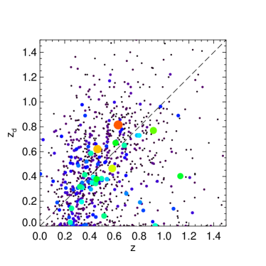
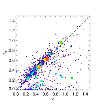
Figure 11.— Tomographic redshift versus real redshift for noisy (left) and noiseless (right) data. The colors and sizes of the points reflect the detection significance of the cluster. The fraction of clusters with tomographic redshift errors $|\Delta z|\leq 0.2$ is $45\%$ and the root mean square deviation from the real redshifts is $\langle(\Delta z)^{2}\rangle^{1/2}=0.41$ (see Table 5).

In Figure 11 we show scatter plots of tomographic redshift, $z_{d}$, versus real redshift where again points are colored according to their detection significance and higher likelihood points are larger. The left panel includes noise while the right panel is for noiseless data. The filter profile $G(\theta)$ used to determine the tomographic redshift (see eqn. 16) was the truncated NFW profile with $\theta_{\rm s}=0.50^{\prime}$ and $\theta_{\rm out}=5.5^{\prime}$, which detected more clusters than the others. For noisy weak lensing data, $45\%$ of clusters have tomographic redshifts with $|\Delta z|\ \leq 0.2$, where $\Delta z\equiv z_{\rm real}-z_{d}$. The rms deviations from the real redshifts are $\sigma_{\Delta z}\equiv\langle(\Delta z)^{2}\rangle^{1/2}=0.41$. For the ideal case of no noise these numbers change to $67\%$ within $|\Delta z|\leq 0.2$ and $\sigma_{\Delta z}=0.34$. The reliability of the tomographic redshifts for the noiseless case reflect the intrinsic limitations of this effectively two dimensional method. The broad lensing kernel and projections of large scale structure limit the accuracy to which radial positions can be determined.

From the colors and sizes of the points in Figure 11 it is clear that tomographic redshifts are more accurate for clusters with a higher detection significance. In Figure 12 we show scatter plots of redshift error $\Delta z$ versus detection significance, which illustrates that the redshift errors taper down dramatically for more significant detections. If there were a candidate ‘dark clump’ corresponding to a very high peak in a likelihood map, the tomographic redshift might provide the redshift of the cluster reasonably well, and would be the only means available to determine a redshift in the absence of a significant overdensity of galaxies. However, we saw in §3.2 that $\sim$ 15 % of the most significant peaks were projections, so there would be no guarantee that the object was an actual cluster, although the tomographic redshift information could be taken into account when devising a strategy for follow up.

Scatter plots of the redshift error $\Delta z$ versus mass and redshift are shown in Figure 13 and Figure 14. As expected, the tomographic redshift errors decrease for more massive clusters and for clusters closer to the peak of weak lensing kernel ($\sim 0.4$). However, the likelihood of the detection is clearly a better indicator of the tomographic redshift reliability than mass or redshift, since the strength of the lensing signal is determined by both the mass and redshift of a cluster.

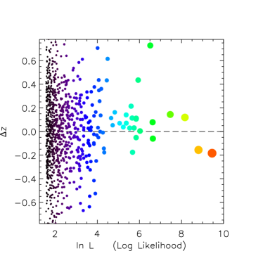
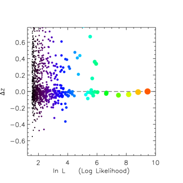
Figure 12.— Tomographic redshift errors versus likelihood for noisy (left) and noiseless (right) data. The colors and sizes of the points reflect the detection significance of the cluster.

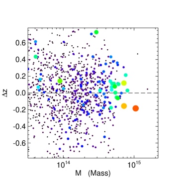
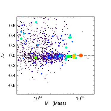
Figure 13.— Tomographic redshift error versus cluster mass for noisy (left) and noiseless (right) data. The colors and sizes of the points reflect the detection significance of the cluster.

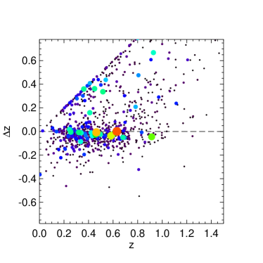
Figure 14.— Tomographic redshift error versus cluster redshift for noisy (left) and noiseless (right) data. The colors and sizes of the points reflect the detection significance of the cluster. The linear feature in the upper left corner of the plots are an artifact of a slight tendency for the tomography to map low signal no noise detections to $z_{\rm d}=0$, hence $\Delta z=z$.

6.2. Tests of Tomography

The truncation scale $\theta_{\rm out}$ in eqn. (34) that optimizes the number of clusters detected is not necessarily optimal for minimizing the error $\Delta_{z}$ of tomographic redshifts $z_{d}$ of the clusters. We applied the TMF to our sample of clusters with truncation scales $\theta_{\rm out}=3.0^{\prime},10.0^{\prime},15.0^{\prime}$ and found negligible improvement in the tomographic redshift errors.

Finally, we quantify the degree to which tomographic redshifts depend on the assumed model cluster profile $G(x)$ in eqn. (16), by computing tomographic redshifts for the same sample of clusters but using a different shear profile. We consider an isothermal sphere with a core, where the core radius is set to the same value of $\theta_{\rm s}=0.50$ used for the NFW scale radius profile and we adopt a Gaussian truncation scale of $\theta_{\rm out}=5.5$. An isothermal sphere with a core has tangential shear profile

$$G_{\rm ISO}(x)=\frac{1+\frac{1}{2}x^{2}}{(1+x)^{3/2}},$$ (36)

(Blandford & Kochanek 1987) with $x=\theta/\theta_{\rm s}$. This profile has an outer power law slope of $\sim\theta^{-1}$, different from the $\sim\theta^{-2}$ scaling of the NFW profile used with the TMF. Overall, the isothermal profile gives tomographic redshift errors similar to the NFW profile used in this section, although for a particular cluster the redshifts deduced can be different.

Table 5 summarizes the results of this section on the reliability of tomographic redshifts, and its dependence on truncation scale and filter profile shape.

Table 5Tomography Tests

	Noisy		Noiseless
Filter	$\left|\Delta z\right|\ \leq 0.2$	$\sigma_{\Delta z}$	$\left|\Delta z\right|\ \leq 0.2$	$\sigma_{\Delta z}$
NFW $\theta_{\rm out}=3.0$	42%	0.44	67%	0.36
NFW $\theta_{\rm out}=5.5$	45%	0.41	67%	0.34
NFW $\theta_{\rm out}=10.0$	46%	0.40	67%	0.35
NFW $\theta_{\rm out}=15.0$	47%	0.39	66%	0.36
Isothermal $\theta_{\rm out}=5.5$	46%	0.40	65%	0.35

NOTES.— Summary of tests on accuracy of tomographic redshifts. The column labeled indicates the filter used, and the left and right columns indicate the fraction of clusters with $|\Delta z|\leq 0.2$ and the variance of the tomographic redshifts $\sigma_{\Delta z}$ for noisy and noiseless mock sources.

7. Discussion

We have described a fast efficient simulation scheme for computing the statistics of shear selected galaxy clusters from weak lensing. By tiling the line of sight with 32 unique PM simulations, our algorithm is unique in that it densely samples the primordial Gaussian distribution of random phases of large scale structure along the light cone, providing an accurate representation of the statistics of rare events. We have confirmed that the two point statistical properties of the three dimensional density field (Figure 1) and the abundance of galaxy clusters in the light cone (Figure 2) are accurately reproduced. Although the dynamic range of our PM simulations is limited, we argued that high resolution simulations are not necessary to study shear selected cluster because of the small scale shot noise limit of weak lensing observations.

A maximum likelihood tomographic technique was presented which utilizes the photometric redshifts of source galaxies to determine the radial position of a galaxy cluster from weak lensing alone. We introduced a tomographic matched filtering (TMF) shceme, which optimally incorporates this additional radial information to detect more clusters. We applied the TMF to a large ensemble of simulations and found that it enhances the number of clusters detected with $S/N\gtrsim 4.5$ by as much as $76\%$ (see Table 4 and 8). As illustrated by Figure 8, the TMF increases the dynamic range of weak lensing searches for clusters, detecting more high redshift clusters and extending the mass sensitivity down to the scale of large groups. Furthermore, binning the sources coarsely using only three redshift bins was sufficient to reap the benefits of tomography. Thus the filtering scheme developed here can be applied to ground based weak lensing observations in as few as three bands, since two colors and a magnitude provide enough information to bin sources this crudely.

For the case where the photometric redshifts of sources are known more precisely, as could be achieved with multicolor ground based data, we quantified the errors in the tomographic redshifts. For the densities of sources used in this paper, $45\%$ of clusters detected with signal to noise ratio $S/N\gtrsim 4.5$ had tomographic redshift errors $|\Delta z|\leq 0.2$ and the rms deviation from the real redshifts is $\sigma_{\Delta z}=0.41$, with smaller errors for higher $S/N$ ratios.

The most appealing property of shear selected cluster samples in comparison to other methods of detecting clusters, is that the expected cluster distributions can be reliably determined for any cosmological model using simulations like those described in this paper. Because on the scales of interest only gravity is involved, comparing theory to observations does not, in principle, depend on assumptions about the relationship between dark and luminous matter. However, in practice projection effects and incompleteness are likely will complicat the interpretation of shear selected samples.

Weak lensing searches for clusters are plagued by projection effects. In particular, we found that the maximum intrinsic efficiency of weak lensing cluster surveys is $\sim 85\%$. Phrased in terms of our criteria for matching peaks with clusters (§2.5), of order $\sim 15\%$ of the most significant peaks detected in noiseless weak lensing maps do not have a collapsed halo with $M>10^{13.5}\ h^{-1}{\rm\ M}_{\odot}$ within a $3^{\prime}$ aperture. This intrinsic inefficiency, also noted by previous investigators (White, van Waerbeke, & Mackey 2002; Padmanabhan, Seljak, & Pen 2003; Hamana, Takada, & Yoshida 2003), arises because of the broad weak lensing kernel and confusion from large scale structure fluctuations.

The calculated maximum intrinsic efficiency is sensitive to parameters. Lowering the limiting mass, $10^{13.5}\ h^{-1}{\rm\ M}_{\odot}$, of our cluster catalog, increasing the size of the aperture, $3^{\prime}$, used to correlate peaks with halos, or reducing the linking length, $b=0.2$, of the FOF group finder, would all increase the efficiencies deduced. Nevertheless, some of the most significant peaks in the mass maps do not correspond to actual clusters. While cluster finding in numerical simulations involves applying a group finding algorithm to 3-d dark matter particle distributions, observationally determining whether there is a galaxy cluster at the location of a given peak will depend on observational criteria like the overdensity of galaxies, X-ray flux, SZ decrement, or the presence of a brightest cluster galaxy. Thus, any criteria employed to distinguish the real clusters from the projections will rely on detecting baryons. Because our ability to detect these baryons is a function of mass and redshift, and because of the scatter between baryonic observables and the underlying mass of the dark matter halo, the projection effects in weak lensing searches will degrade the well defined selection function deduced from ‘dark matter only’ simulations like those employed in this work.

In the context of using cluster counts to constrain cosmological parameters, the uncertainties in the selection function caused by projections are exacerbated by the high incompleteness of shear selected cluster samples. Even for an efficiency cut of $e\geq 60\%$, the completeness is $\gtrsim 50\%$ only for the most massive clusters $M\gtrsim 10.0^{14.3}$ which are near the peak of the lensing kernel at $z\sim 0.3$, and lower everywhere else. The severe projection effects imply that these missed clusters are likely to scatter in or out of the detected sample. In light of the fact that this number of missed clusters is of the same order as the number detected, an accuracy of $x\%$ in the final cluster sample requires a theoretical understanding the selection function to better than $\sim x\%$. This is likely to be very hard. One alternative is to throw away the number count information and use only the shape of the redshift distribution of shear-selected clusters to constrain cosmology since the shape will be much less sensitive to the precision to which the selection function is known.

Cross correlation of shear selected cluster samples with overlapping optical, SZ, or X-ray cluster catalogs is an important cosmological application (Schirmer et al. 2003,2004; Hughes et al. 2004). For such a cross-correlation it is likely to be advantagous to work at lower efficiency thresholds, considering that the number of clusters per square degree for an efficiency $e\geq 60\%$ is five times larger than that with $e\geq 75\%$ (see Table 4). These less significant peaks will span a larger mass and redshift range increasing the amount of overlap between the two cluster samples. Besides addressing probable baryonic biases for baryon selected clusters, cross correlation could be the most expedient route to precision cosmology with cluster surveys. In order to recover parameter sensitivity degraded by the scatter in the mass-observable relations, Majumdar & Mohr (2003) advocate calibrating these relations with extensive follow up mass measurements of a fraction of the clusters in a ‘baryon selected’ sample. An alternative to such a follow up campaign of individual clusters is to conduct a parallel weak lensing survey, and use the clusters detected from both weak lensing and, say SZ, to determine the mass-observable relation statistically. Because the mass and redshift distributions of the shear selected clusters is known for any cosmological model, the distribution of dual weak lensing-SZ detections can be used to simultaneously constrain cosmology and the relationship between mass and SZ decrement. In addition to the statistical mass-SZ decrement calibration provided by the distribution of dual detections, stacked weak lensing mass measurements of the individual SZ clusters can be used to provide another constraint on this relation. Finally, it is worth emphasizing that an optical cluster search (Postman et al. 1996; Kepner et al. 1999; Gladders & Yee 2000; White & Kochanek 2002; Kochanek et al. 2003) could be conducted using the same deep imaging data used to measure weak lensing. Indeed, Schirmer et al. (2003, 2004) have already combined shear selection with optical color selection, and confirmed several color-selected optical cluster candidates with weak lensing. Such parallel analyses of shear-selected cluster samples and baryonic cluster samples will provide mass calibration, help break parameter degeneracies, and eliminate systematics inherent in cluster surveys.

The potential of shear selected clusters to provide precision constraints on the dark energy, either alone or in conjunction with another baryonic cluster survey, are topics which merit future investigation.

References

- Allen, Schmidt, & Bridle (2003) Allen, S. W., Schmidt, R. W., & Bridle, S. L. 2003, MNRAS, 346, 593
- Bacon & Taylor (2003) Bacon, D. J. & Taylor, A. N. 2003, MNRAS, 344, 1307
- Bahcall & Fan (1998) Bahcall, N. A. & Fan, X. 1998, ApJ, 504, 1
- Bartelmann & Schneider (2001) Bartelmann, M. & Schneider, P. 2001, Phys. Rep., 340, 291
- Bartelmann, Perrotta, & Baccigalupi (2002) Bartelmann, M., Perrotta, F., & Baccigalupi, C. 2002, A&A, 396, 21
- Navarro, Frenk, & White (1997) Navarro, J. F., Frenk, C. S., & White, S. D. M. 1997, ApJ, 490, 493
- Berlind, Narayanan, & Weinberg (2000) Berlind, A. A., Narayanan, V. K., & Weinberg, D. H. 2000, ApJ, 537, 537
- Berlind, Narayanan, & Weinberg (2001) Berlind, A. A., Narayanan, V. K., & Weinberg, D. H. 2001, ApJ, 549, 688
- Bernstein & Jarvis (2002) Bernstein, G. M. & Jarvis, M. 2002, AJ, 123, 583