Distant field BHB stars and the mass of the Galaxy II: Photometry and spectroscopy of UKST candidates $16<B<19.5,11<R<52$ kpc

Abstract

This is the second in a series of papers presenting a new calculation of the mass of the Galaxy based on radial velocities and distances for a sample of faint $16<B<21.3$ field blue horizontal-branch (BHB) stars. We present accurate $BV$ CCD photometry and spectra for 142 candidate A–type stars selected from $ub_{j}r$ photometry of UK Schmidt telescope plates in six high–Galactic–latitude fields. Classification of these candidates produces a sample of 60 BHB stars at distances of 11–52 kpc from the Sun (mean 28 kpc), with heliocentric line-of-sight velocities accurate to 15 km s^-1, and distance errors $<10\%$. We provide a summary table listing coordinates and velocities of these stars. The measured dispersion of the radial component of the Galactocentric velocity for this sample is 108 $\pm$ 10 km s^-1, in agreement with a recent study of the distant halo by Sirko and coworkers. Measurements of the Ca II K line indicate that nearly all the stars are metal-poor with a mean [Fe/H] = -1.8 with dispersion 0.5. Subsequent papers will describe a second survey of BHBs to heliocentric distances $70<R<125$ kpc and present a new estimate of the mass of the Galaxy.

1 Introduction

In contrast with the detailed knowledge we have of the stellar content of the halo of the Galaxy, the dark matter content is far less well characterised, with both the total mass and the size of the halo poorly determined quantities. The accurate measurement of the mass profile would provide important clues to the nature of the dark matter. For instance, an accurate estimate of the mass within a radius of 50 kpc is required to establish the fraction of the mass in compact objects identified from microlensing experiments (e.g Alcock et al. 2000). Quantifying the distribution of dark matter in the Galaxy is essential for understanding the assembly of the various baryonic components through comparison with simulations. This paper is the second in a series of four, presenting a new measurement of the mass profile of the Galaxy out to the largest radii, $r>100$kpc, using surveys for remote halo blue horizontal branch (BHB) stars.

The main shortcoming of previous analyses of the mass of the Galaxy is the small size of the sample of objects at large radii, used as dynamical tracers. Wilkinson and Evans (1999, hereafter WE99) calculate the total mass of the Milky Way to be $M_{tot}=1.9^{+3.6}_{-1.7}\times 10^{12}M_{\odot}$, using the full set of 27 known satellite galaxies and globular clusters at Galactocentric radii $r>$ 20 kpc (six of which possess measured proper motions). This sample must be nearly complete, so a new population of distant halo objects must be found in order to increase the number of dynamical tracers. Field BHB stars are ideal for this purpose. These A–type stars are luminous, $M_{V}=0.9$ (§5), which ensures that they can be detected to large distances, and have a small spread in absolute magnitude, so their distances may be determined accurately.

In a recent paper Sakamoto et al. (2003) added new kinematic data to the dataset used by WE99, and obtained a considerably more precise estimate of the total mass of the Galaxy of $M_{tot}=2.5^{+0.5}_{-1.0}\times 10^{12}M_{\odot}$. Primarily, the new kinematic data comprise radial velocities of 412 BHB stars, of which 211 have proper motions, at heliocentric distances $R<10$kpc, with a median distance of $\sim$ 4.5kpc. Sakamoto et al. adopted the WE99 mass model, where the total mass enclosed within Galactocentric radius $r$ is $M(r)=M_{tot}/(1+a^{2}/r^{2})^{1/2}$. Here $a$ is the scale length, for which the best-fit value of 225kpc was obtained. For $r=20$kpc, i.e. a radius containing all the BHB stars used in the analysis, this gives $M(r)=0.09M_{tot}$. This indicates that most of the improved precision derives from kinematic data within a radius containing only one tenth of the total mass, and therefore relies on extrapolation of a model that is tightly constrained only at small radii. In a review of mass estimates of the Milky Way halo, Zaritsky (1999) emphasises the dangers of such extrapolation (see also Bellazzini, 2004, for a useful discussion). This motivates a new survey for remote BHB stars, at distances that are a substantial fraction of the halo scale length $a$, in order to obtain a direct measure of the enclosed mass at large radii.

Although BHB stars are abundant in the Galaxy halo, selection of a clean sample is not straightforward. Samples of field A–type stars in the halo are easily identifiable in UBR (or equivalent e.g. $ugr$) multicolour datasets (e.g. Yanny et al. 2000). Samples selected by broadband colour include not only BHB stars but also stars of main sequence surface gravity that are some 2 magnitudes less luminous, predominantly field blue stragglers (hereafter A/BS), as well as a small proportion of quasars. The reason that no large sample of remote $r>30$kpc BHB stars has yet been compiled, is that the methods developed for separating the two populations of A stars (e.g. Kinman, Suntzeff, and Kraft, 1994) require signal-to-noise ($S/N$) ratios that are unfeasibly high for such faint stars ($B>18$). In the first paper in this series (Clewley et al. 2002, hereafter Paper I), we developed two methods that overcome the difficulties. The methods require relatively modest telescope resources, yet produce samples with high completeness and low contamination. The methods are applicable specifically to the classification of halo stars with strong Balmer lines, defined by EW $H\gamma>13$Å, i.e. A stars in the approximate colour range $0.0<(B-V)_{0}<0.2$.

Both methods employ a Sersic function fit to the H$\gamma$ and H$\delta$ absorption lines. The first method, the $D_{0.15}$–Colour method, plots the average of the width of the two Balmer lines against $(B-V)_{0}$ colour. The A/BS stars, having higher surface gravity, separate from the BHB stars because of their broader Balmer lines. The EW of the CaK line is used to filter out a small number of interlopers in the BHB sample. We used Monte Carlo methods to establish that with $(B-V)_{0}$ colours accurate to $0.03$ magnitudes, and spectra of $S/N=15{\rm\AA}^{-1}$, samples of BHB stars selected by this method would be about $87\%$ complete, with a contamination of $7\%$ by A/BS stars. Contamination at this level can safely be accounted for in the dynamical analysis. Spectra of this $S/N$ are also suitable for measurement of the radial velocities. The second method, called the Scale width–Shape method, plots two parameters of the Sersic fit, the scale width $b$, against the power–law exponent $c$. The method is almost as efficient as the $D_{0.15}$–Colour method, with $82\%$ completeness and $12\%$ contamination, for the same spectroscopic $S/N$ of $15{\rm\AA}^{-1}$. Again, the EW of the CaK line is used to filter out a small number of interlopers. The advantage of the Scale width–Shape method is that colours are not needed. For samples of stars with existing accurate $(B-V)_{0}$ colours, the first method is preferred, as the contamination is lower, and the completeness higher. The gain is small, however, and accurate photometry is time consuming. Where accurate colours are not already available, if telescope resources are limited, the best practical solution will be simply to obtain spectra, and use the Scale width–Shape method.

In this second paper we describe the compilation of a sample of BHB stars in the magnitude range $16<B<19.5$, corresponding to heliocentric distances $11<R<52$ kpc, using the two classification methods described above. This first survey (hereafter the UKST survey) starts from photographic plates taken with the United Kingdom Schmidt Telescope (UKST). In the third paper we describe a second survey, for fainter BHB stars, $20<g*<21.1$, corresponding to heliocentric distances $70<R<125$ kpc. This second survey starts from the Sloan Digital Sky Survey (SDSS) Early Data Release (EDR) (Stoughton et al. 2002). The fourth paper will present the dynamical analysis of these two data sets, combined with the 27 satellites and globular clusters analysed by WE99.

The layout of the remainder of the paper is as follows. In section 2 we describe the selection of the UKST fields, the reduction of the plate scans, and the production of the multicolour photometric datasets. We provide catalogues of a total of 461 objects with the colours of A–type stars, which are candidate halo BHB stars. Section 3 covers CCD $B-V$ photometry of 280 candidate BHB stars, and section 4 describes the spectroscopic observations of 156 candidates. We describe the measurement of the metallicity and the radial velocity from the spectra. Section 5 reviews the measurement of distances of BHB stars. In Section 6 we use these results and the methods developed in Paper I to classify these stars, and we provide a table of distances and radial velocities of the 60 confirmed BHB stars. Finally, in Section 7 we provide a summary of the main conclusions of the paper.

2 The selection of BHB candidates

In this section we explain how the six UKST fields for the survey were chosen, and we describe the compilation of calibrated three-band photographic photometric datasets in each field. We detail the (dereddened) magnitude and colour criteria for the selection of candidate BHB stars from these datasets, and provide complete lists of the candidates for each field. These candidate lists are suitable, for example, for quantifying number counts of A–type stars in different directions through the Galaxy. On the other hand, the sub-set of objects for which CCD photometry and spectroscopy were obtained was not selected randomly from the candidate lists. Rather, both magnitude and colour criteria were applied. For example, for the CCD photometry, if the seeing was poor, brighter objects were selected for observation, while spectroscopy was limited almost exclusively to objects with confirmed CCD colours in the range $-0.05<(B-V)_{0}<0.25$, since the classification methods work well only within this range. In fact, because the colour selection criteria were not finalised at the outset of the survey, a small number of objects that fall outside the selection criteria used to define the complete candidate samples, were also included in the CCD photometry and spectroscopy campaign. The consequence of this is that the final list of confirmed BHB stars is not a random sub-set of the complete candidate lists, and so cannot be used, for example, for quantifying the density profile of BHB stars in the halo. On the other hand, since the stars have been selected without reference to kinematic information, each confirmed BHB star randomly samples the radial–velocity distribution function at that distance, and so the sample is suitable for dynamical analysis.

2.1 Field selection

We selected the fields to give good coverage in opposing directions above and below the Galactic plane, with a wide range of Galactic longitudes. Although the kinematic information is limited to radial velocities, because of the offset of the Sun from the Galactic centre the widely different lines of sight through the Galaxy provide some complementary information on the anisotropy of the stellar orbits, and also avoid the risk of the whole sample residing in a halo stream, such as those associated with the Sagittarius dwarf galaxy (e.g. Ibata, Gilmore & Irwin, 1994, Dohm-Palmer et al. 2001, Newberg et al. 2002). The selection of fields was subject to the availability of suitable plate material in the UKST archive. This restricts the search to negative declinations, and to fields containing pairs of high–grade plates in the $u$, $b_{j}$, and $or/r$ bands. We chose six fields at high Galactic latitude, $|b|\geq 45^{\circ}$, to minimise Galactic extinction. The coordinates of the centres of the six fields are provided in Table 1, and plotted in Fig. 1.

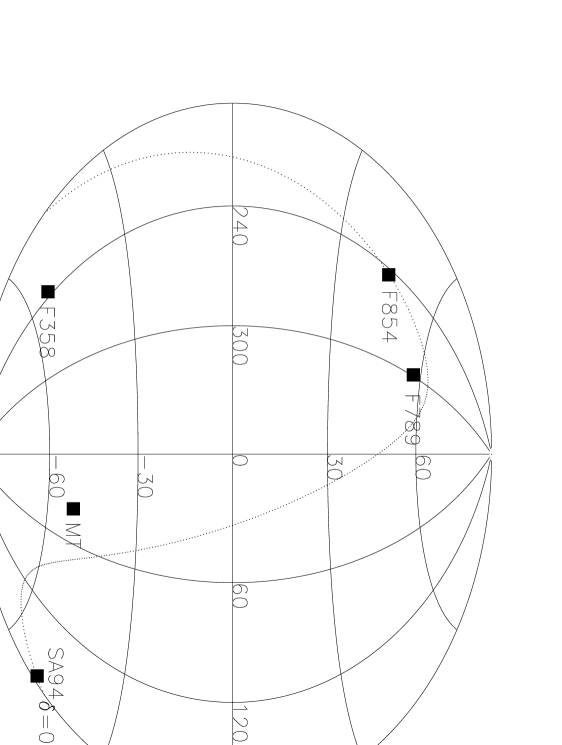
Figure 1: Galactic coordinate Aitoff projection showing the locations of the six survey fields. The fields were chosen to sample different directions through the Galaxy, within the constraints imposed by the availability of suitable plate material in the UKST archive. High Galactic-latitude fields were chosen to minimise extinction. The dotted line plots zero declination.

Field name	l	b	RA	Dec
			J 2000
SGP	250	-89	0 55	-27 47
SA94	175	-50	2 53	0 12
F358	236	-54	3 38	-34 50
F854	244	45	10 23	-0 15
F789	299	58	12 43	-5 16
MT	37	-51	22 06	-18 39

Table 1: Galactic and equatorial coordinates of the centres of six fields observed in the survey, ordered by Right Ascension.

Field	Area	Reddening	Sample $b_{j}$	Sample $b_{j}$	No.
	(sq. deg.)	$\langle E(B-V)\rangle$	range (red)	range (unred)	cand.
SGP	24.8	0.018	$18.47-19.77$	$18.40-19.70$	64
MTF	25.6	0.032	$17.63-19.63$	$17.50-19.50$	128
SA94	25.7	0.067	$16.27-19.97$	$16.00-19.70$	72
F358	23.6	0.011	$17.34-19.74$	$17.30-19.70$	28
F789	25.3	0.029	$15.32-19.02$	$15.20-18.90$	114
F854	25.3	0.048	$16.19-19.59$	$16.00-19.40$	55

Table 2: Data for the six fields in the survey. Listed are the effective area of each field, the mean reddening, $\langle E(B-V)\rangle$, the range of $b_{j}$ magnitudes with and without the reddening correction and the total number of candidate stars in each field.

2.2 Compilation of uncalibrated three-band photographic photometric datasets

Pairs of photographic plates in each of the three bands were scanned by the Automated Plate Measuring (APM) machine (Kibblewhite et al. 1984) to produce lists of detected objects, and their measured properties, including uncalibrated fluxes. These lists were then matched and calibrated.

In four fields we used pairs of plates in the $u$, $b_{j}$, and $or$ pass-bands. The exceptions were F358 which had a single $or$ plate, and SA94 where we used two $r$ plates. The $r$ band is a slightly narrower and redder band than the standard $or$ band. The effective area of the scan in each field, approximately 25 square degrees, is listed in Table 2. The effective area is the actual area scanned, after allowing for regions drilled out around bright stars, multiplied by a factor 0.8 to account for incompleteness due to plate flaws, satellite trails and merging with neighbouring images. The survey covers a total effective area of 150.3 square degrees over the six fields.

In pairing and calibrating the object lists from the plates in each field we followed the same reduction steps described in detail by Warren at al. (1991) – in fact the SGP catalogue described here is the same catalogue used by them to search for quasars. In outline, the processing steps are as follows. For each detected object the APM measures a parameter intensity that scales monotonically and non–linearly with flux, as well as several parameters describing the light profile and the shape of each source. The variation of the light profile as a function of intensity, for stellar objects on the plates, is used to calibrate the intensities onto a scale that is approximately linear with flux (Bunclark & Irwin, 1983). The main purpose of using pairs of plates in each band was to reduce the photometric uncertainties by averaging the intensities. The response curve of the photographic emulsion is not perfectly uniform, but varies across each plate (known as field effects). In matching plates taken in the same filter we gridded the area scanned, and calibrated the intensity scale of the second plate to the scale of the first plate in each patch i.e. we forced the field effects on the second plate to match those on the first plate. A similar procedure was adopted in order to match the object catalogues from different passbands. The $b_{j}$ band was adopted as the reference passband and any field effects in the other photometric bands were forced to match any field effects present in the $b_{j}$ band.

We used the shape and light profile information to classify the objects as stellar and non–stellar, combining the information from all the plates in order to improve the discrimination. Finally we converted the intensities to a logarithmic scale and calibrated to magnitudes using CCD observations of several stars on each plate, as described below.

2.3 Calibration

For the calibration we made CCD observations in the $U$, $B$, and $R$ bands of selected fields. We also used the CCD $BV$ photometry of the candidates themselves (i.e. all A-type stars). We created $U$ and $R$ sequences from the A–star $BV$ photometry using the relations: $U-B=0.5(B-V)$, for 0 $<(B-V)<$ 0.2; $B-R=0.02+1.51(B-V)$ for $(B-V)<1.0$. The $UBR$ photometry was then converted into the $u,b_{j},or,r$ natural system of the UKST using the relations,

$$u=U-0.01-0.01\,(U-B)\>\>\mathrm{for}\>-1.4<U-B<2.0,$$

$$b_{j}-B=0.01-0.18\,(B-R)\>\>\mathrm{for}\>0.0<B-R<1.6,$$

$$or-R=0.00-0.01\,(B-R)\>\>\mathrm{for}\>0.0<B-R<1.6,$$

$$r-R=-0.01-0.06\,(B-R)\>\>\mathrm{for}\>0.0<B-R<1.6.$$

The number of stars which defined the calibration curve in any band was typically 25. The colour equations quoted above are either taken from Warren et al. (1991), or they were computed using the procedures described there.

Bearing in mind the earlier discussion of field effects, in establishing the photometric errors there are two terms to consider. There are random errors, which can be assessed for any band from the scatter in a plot of magnitude difference between the two plates as a function of magnitude (Warren et al. 1991, Fig. 3). There are also systematic errors, due to field effects on the reference plate in the $b_{j}$ band, and these are the same in all passbands, due to the way in which the field effects in all plates were forced to match those on the reference $b_{j}$ plate. These systematic errors do not contribute to the uncertainties in the colours. They are larger than the random errors over the magnitude range of interest and were quantified by measuring the scatter in the calibration curves. Table 3 summarises the photometric uncertainties in the photographic catalogues.

$b_{j}$	$\sigma(b_{j})$	$\sigma(u-b_{j})$	$\sigma(b_{j}-or)$
16	0.11	0.05	0.05
17	0.11	0.05	0.05
18	0.11	0.05	0.05
19	0.11	0.06	0.06
20	0.11	0.09	0.10

Table 3: Uncertainties for the photographic photometric data as a function of $b_{j}$ magnitude. The reason why the magnitude errors are larger than the colour errors is explained in the text.

Star	R.A. (J2000.0)	Dec. (J2000.0)	$b_{j}$	$u-b_{j}$	$b_{j}-or$	$\sigma(u-b_{j})$	$\sigma(b_{j}-or)$
CSGP-001	01 05 28.20	-26 14 00.79	19.40	0.11	0.10	0.07	0.08
CSGP-002	01 03 35.32	-25 54 49.64	19.05	-0.03	0.11	0.06	0.06
CSGP-003	01 02 44.21	-26 27 46.75	18.87	0.16	0.34	0.06	0.06
CSGP-004	01 02 35.56	-26 12 39.58	18.52	0.08	0.45	0.06	0.06
CSGP-005	01 01 56.71	-25 38 03.13	18.63	0.16	0.19	0.06	0.06
CSGP-006	01 01 44.02	-26 58 32.59	19.55	0.07	0.31	0.08	0.08
CSGP-007	00 59 23.47	-25 48 36.96	19.56	0.20	0.22	0.08	0.08

Table 4: Photometric catalogue of A-type stars selected from six UKST fields shown in Figure 2. The photometric uncertainties in these estimates are interpolated from those in Table 3. This table is presented in its entirety in the electronic edition of Monthly Notices. A portion is shown here for guidance regarding its content and form.

Figure 2: Two-colour diagrams for the stellar targets for the six fields listed in Table 1. The selection box defines the complete sample of candidate BHB stars. The number of stars in each box, their magnitude range and reddening correction are listed in Table 2.

2.4 Candidate selection

Figure 2 shows two–colour $u-b_{j}$, $b_{j}-or/r$ diagrams for the stellar objects in each field, and the selection boxes which define the samples of candidate BHB stars. This box is slightly different for each field because we have allowed for Galactic reddening, since the targets are at large distances. In considering candidate selection, the $r$ band is treated as identical to the $or$ band. This is because A stars have colours close to zero, so the difference between the $r$ and $or$ magnitudes for A stars, i.e. the product of a small colour and a small colour term, may be neglected. Similarly the the difference in the extinction correction is negligible, because the reddening in these fields is small (Table 2), and the wavelength difference between the bands is also small. In this subsection all equations involving the $or$ band apply also to the $r$ band.

The selection box is defined by the unreddened colours as follows:

$$\hskip 71.13188pt-0.15<(u-b_{j})_{0}<0.25,$$

$$-0.05<(b_{j}-or)_{0}<0.45,$$

$$(u-b_{j})_{0}-(b_{j}-or)_{0}>-0.40.$$

The $(u-b_{j})_{0}$ cut eliminates objects with large ultraviolet excesses from the sample, such as quasars or white dwarfs. The $(b_{j}-or)_{0}$ cut minimises contamination by F stars. An additional diagonal cut is made because the colour box lies closest to the stellar sequence in this corner. Converting $b_{j}-or$ to $B-V$ using $B-V=-0.02+0.80(b_{j}-or)$ the corresponding range in $B-V$ is $-0.06<B-V<(0.18-0.34)$, where the range in the red limit is a consequence of the diagonal cut (seen in Figure 2). Since we are interested in BHB stars, which have $0.0<B-V<0.20$, the incompleteness introduced by the diagonal cut itself will be negligible.

For each field we shifted the selection box along the reddening vector by an amount appropriate for the value of $E(B-V)$. The mean reddening values for each field, $\langle E(B-V)\rangle$, are provided in Table 2, measured from the extinction maps of Schlegel, Finkbeiner & Davis (1998). We used the reddening relations $E(u-b_{j})=1.40E(B-V)$, and $E(b_{j}-or)=1.36E(B-V)$ (note that the reddening vector is nearly diagonal). The relation between extinction and reddening for the $b_{j}$ band is $A(b_{j})=4.035E(B-V)$. The magnitude range of the candidates is different for each field and is listed in Table 2 together with the number of candidates. The total number of candidates is 461. A catalogue of the candidate A-type stars containing their $b_{j}$ magnitude, $b_{j}-or$ and $u-b_{j}$ colours and their associated errors is provided in Table 4. The stars in this sample are prefixed with a ‘C’, standing for ‘complete’ sample.

The photometric calibration observations were, in fact, obtained as the survey progressed, and the candidate BHB stars had to be selected before the calibration stage. This was possible because the clump of A-type stars is clearly defined, and because the APM intensities are nearly linear with flux. The consequence of this is that some stars observed photometrically or spectroscopically fall just outside the selection boxes.

In F854 we noted a significant faint over-density of fainter ($b_{j}$ = 20.2) BHB candidate stars in the direction $l=244^{\circ}$, $b=42^{\circ}$. We later realised these mark the location of the dwarf spheroidal galaxy Sextans, which resides at a heliocentric distance of 83 kpc. In fact the magnitude limit of our complete sample in this field is 19.59, so the complete sample is not contaminated by Sextans. But it highlights the effectiveness of using Schmidt plates to discover BHB stars out to at least 80 kpc.

3 Photometry

3.1 Observations

The $D_{0.15}$–Colour method of classification requires $B-V$ colours accurate to 0.03 magnitudes, so the photographic photometry of Table 4 is insufficient. To achieve a higher degree of photometric accuracy, $BV$ CCD observations were made of candidate BHB stars drawn from Table 4. We made a total of 421 observations of 280 stars over 47 photometric nights during the period 1998 to 2001. As a rule, the redder objects in the selection boxes shown in Fig. 2 were given lower priority for observation, since this region will contain fewer objects in the desired colour range $0<(B-V)_{0}<0.2$. The observing dates are listed in Table 5. Three telescopes were used for the photometry. (i) The 1.0-m Jacobus Kapteyn Telescope (JKT) at La Palma. We used a TEK1 1024x1024 CCD detector for the 1998 observing run, which was replaced by a SITe2 2048x2048 CCD for subsequent runs. Each chip has a scale of 0.33” pixel^-1. (ii) The 2.5-m Isaac Newton Telescope (INT) at La Palma, using Chip 4 of the Wide Field Camera, which is an EEV42-80 4096x2048 CCD with a scale of 0.33” pixel^-1. (iii) The ANU 2.3-m Telescope at Siding Spring observatory (SSO), Australia, using a SITe 1024x1024 CCD with a pixel scale of 0.59” pixel^-1. Generally the brighter stars were observed at the JKT and the fainter ones at the SSO and INT. Repeat observations were made between telescopes, in order to establish the external errors.

Throughout each night we observed typically 30 standard stars from Landolt (1992). The standards were chosen to span a large range in colour, and were observed over a wide range of airmass. Extinction and colour terms were measured every night. The target A-type stars were observed as near to the meridian as possible, typically at airmasses $\leq$ 1.3. The integration times for each exposure were adjusted, dependent on the brightness of the star, the brightness of the sky, and the seeing, with the aim of achieving uniform $S/N$ for all objects.

3.2 Data reduction, analysis, and results

Data reduction techniques employed standard routines available in IRAF (V2.11) for bias, flat-field correction, and the removal of cosmic rays. The data taken on the ANU 2.3-m SSO telescope was reduced and analysed using FIGARO. Twilight sky exposures were used to flat-field the data, and a correction was then applied to account for the large-scale gradient in the sky. The correction frames were created by combining and smoothing uncrowded flat-fielded image frames, from which the stars were $\sigma-$clipped. This procedure will, in fact, only be correct if any scattered light in the instrument illuminates the CCD uniformly. With hindsight, it would have been best to quantify the scattered light, using a procedure such as that suggested by Manfroid, Selman, and Jones (2001). Systematic errors are discussed below.

Stellar aperture photometry was performed using the APPHOT package in IRAF. For the standards we chose an aperture radius equal to 6.5 times the measured image full-width-half-maximum (FWHM). The seeing was typically 1.2” – 1.6”, giving an aperture radius of $\sim$ 7.8” – 10.4”. The sky level was measured in an annulus between radii of 10 and 20 FWHM. We solved for the nightly $B$ and $V$ extinction and colour coefficients. The typical RMS scatter about the best-fit relations in both $B$ and $V$ filters was 0.015 magnitudes. This is noticeably larger than the Poisson errors, and the excess scatter could be due to scattered light.

Telescope	Date	N	Fields
SSO	1998  Sep 13-16	4	SGP
JKT	1998  Oct 15, 17-20	5	SA94, MTF
SSO	1999  Mar 12-18	7	F854, F789, SGP
JKT	1999  April 4, 7-9	4	F854, F789
SSO	1999  Oct 11-17	7	SGP
JKT	1999  Oct 30-31, Sep 1, 3-5	6	SA94, MTF
SSO	1999  Nov 17-20	4	F358
SSO	2000  Feb 2-4	4	F854, F789
JKT	2000  Mar 23, 26, 28	3	F854, F789
INT	2001  Mar 29-30, Apr 1	3	SA94, MTF

Table 5: The dates and total number of photometric nights ‘N’ for the photometric survey in each of the six fields presented in Table 1. Observations were made using the 1.0-m Jacobus Kapteyn Telescope (JKT), the 2.5-m Isaac Newton Telescope (INT) and the 2.3-m Telescope at Siding Spring Observatories (SSO).

For the survey stars we selected an aperture radius of 2.3 times the average FWHM of stars in each frame. This small radius is close to optimum in terms of $S/N$. To correct to the large aperture used for the standards, we averaged the aperture correction measured for $\sim$ 5 bright, isolated, unsaturated stars in each image frame. The uncertainty on the aperture correction is not negligible, being typically 0.01 magnitudes, and was added in quadrature to the Poisson errors for the survey stars. The resulting $BV$ magnitudes and errors are found by inverting the transformation solutions. The total internal photometric errors for the programme stars with $16<V<20$ respectively are in the range 0.015 - 0.030 magnitudes in $V$ and 0.020 - 0.040 in $B-V$. To obtain an estimate of the size of any systematic errors, due, for example, to scattered light, we have looked at the scatter in the photometry of objects observed on different nights, and on different telescopes.

Range in V magnitude	$N_{obs}$	$N_{stars}$	$\sigma_{V}$	$\sigma(B-V)$
15 $<$ V $<$ 16	24	6	0.021	0.025
16 $<$ V $<$ 17	42	20	0.021	0.021
17 $<$ V $<$ 18	23	8	0.025	0.031
18 $<$ V $<$ 19	85	38	0.029	0.037
19 $<$ V $<$ 20	41	20	0.040	0.042

Table 6: The standard deviation in the value of a single observation of $V$ and $B-V$, as a function of $V$, evaluated from repeat observations in the survey. There are 215 repeat observations of 92 stars.

The external errors for the photometric measurements were determined using the approach of Pearson & Hartley (1976) (see also e.g. Kinman, Suntzeff, and Kraft, 1994; hereafter KSK), which looks at the range of values $R$ (i.e. the difference between the largest and smallest values) in $N$ repeat observations of the same star. The estimate of the external standard deviation, for a single observation, is then given by $\sigma_{ext}={R/k}$, where the coefficient $k$ depends on $N$ (Table 22 of Pearson & Hartley, 1976). Assuming all stars in the same magnitude range have similar errors, we can average the estimate of $\sigma$. For measurements of $n$ stars the estimate of the external standard deviation is given by,

$$\sigma_{ext}=\frac{1}{n}\sum_{i=1,n}\frac{R_{i}}{k_{i}(N_{i})}$$ (1)

where $k_{i}(N_{i})$ is the $k$ factor for star $i$ with $N_{i}$ repeat observations.

We used this approach to compute the errors on $V$ and $B-V$, in 5 magnitude bins. Note that the error on $B-V$ may be smaller than the quadrature sum of the errors on $B$ and $V$, since the $BV$ observations were made quasi–simultaneously, and on closely the same area of the chip, meaning that any systematic errors on the $B$ and $V$ magnitudes may be correlated. Before computing the errors we have to be confident the sample does not contain variable stars, for example RR Lyraes. Previous investigations of large samples of distant A-type stars contain a significant number of variable stars, particularly in the instability strip at $0.2\leq(B-V)_{0}\leq 0.4$. For example, KSK discovered 28 variable stars from a complete sample of 213 A-type stars, and Wilhelm et al. 1999a discovered 56 out of a complete sample of 1000. These studies found very few variable stars in the region $0.0\leq(B-V)_{0}\leq 0.2$ (KSK find 3 stars, Wilhelm et al. 1999a only 2). Accordingly, to compute the errors we limited our analysis to this colour range. Over this colour range we have 92 stars with repeat observations, with a total of 215 observations. Table 6 provides the computed standard deviations, for a single observation, for $V$ and $B-V$, in the 5 magnitude bins. The errors in $V$ computed in this way are about $30\%$ larger than the random errors, and indicate systematic errors contributing to the overall error budget at a level comparable to the random errors. On the other hand the errors in $B-V$ are only slightly larger than the random errors.

We have adopted the values in Table 6 as our error estimates, reducing these values by $\sqrt{N}$, for $N$ repeat observations. Examination of Table 6 reveals that, in order to achieve standard errors in $B-V$ of $<0.03$ magnitudes, at least 2 observations are required for stars fainter than $V=18$. This was achieved for the majority, although not all, of our targets.

The photometric survey resulted in $BV$ observations of 280 stars. The results are provided in Table 7, which for each star lists the name, the equatorial coordinates, the mean unextinguished $V$ magnitude, and unreddened $(B-V)_{0}$ colour, and the uncertainties for these two quantities. Also provided are the value of E($B-V$) used for the extinction corrections, taken from Schlegel et al. (1998), and $N$ the number of repeat observations. We discovered 3 stars with colours $0.2\leq(B-V)_{0}\leq 0.4$ that have large residuals ($\sigma_{(B-V)}\sim$ 0.1). These are candidate variable stars, and have been excluded from the classification process. These three suspected variables are marked with a ‘v’. The number of stars in each field with CCD photometry is listed in Table 8.

Star	R.A. (J2000.0)	Dec. (J2000.0)	$V$	$(B-V)_{0}$	$\sigma(V)$	$\sigma(B-V)$	E$(B-V)$	N
CSGP-003	01 02 44.2	-26 27 46.8	18.69	0.22	0.021	0.026	0.016	2
CSGP-005	01 01 56.7	-25 38 03.1	18.53	0.17	0.017	0.021	0.028	3
CSGP-006	01 01 44.0	-26 58 32.6	19.36	0.17	0.028	0.030	0.018	2
CSGP-009	00 56 03.2	-26 27 30.3	19.13	0.28	0.028	0.030	0.019	2
CSGP-011	00 55 40.7	-26 53 01.8	18.65	0.13	0.021	0.026	0.018	2
CSGP-017	00 47 42.5	-25 47 17.9	19.34	0.12	0.028	0.030	0.015	2
CSGP-018	00 46 00.8	-26 19 38.5	19.36	0.26	0.028	0.030	0.012	2
CSGP-021	00 42 41.7	-26 20 55.6	19.26	0.16	0.028	0.030	0.011	2
CSGP-029	00 58 09.6	-27 23 15.6	19.35	0.11	0.028	0.030	0.020	2

Table 7: Photometric data for the blue horizontal branch star candidates, corrected for extinction. Suspected variables are labelled ’v’. Stars that were subsequently found to be quasars are labelled ’q’. Stars in the complete sample have names prefixed ‘C’, otherwise the stars are prefixed ’I’. This table is presented in its entirety in the electronic edition of Monthly Notices. A portion is shown here for guidance regarding its content and form.

Field name	R.A.	Dec.	Nphot	Nspec
	(J2000.0)
SGP	0 55	-27 47	22	24
SA94	2 53	0 12	34	17
F358	3 38	-34 50	44	8
F854	10 23	-0 15	75	24
F789	12 43	-5 16	63	27
MT	22 06	-18 39	42	56

Table 8: The number of photometric and spectroscopic observations, Nphot and Nspec made in each field. The survey contains photometric measurements for 280 stars. There are 156 stars with spectroscopic measurements.

4 Spectroscopy

4.1 Observations

We obtained medium resolution optical spectra of 156 survey stars over a total of 21 clear nights at the 4.2-m William Herschel Telescope (WHT), La Palma, and the 3.9-m Anglo-Australian Telescope (AAT), Siding Spring Observatory, Australia. The number of stars in each field is provided in Table 8. The dates of the observations are listed in Table 9. The aim was to restrict spectroscopy as far as possible to stars with confirmed CCD colours in the range $0<(B-V)_{0}<0.2$, accurate to better than 0.03 magnitudes, so that we could apply the $D_{0.15}$–Colour classifier. However, because the photometric and spectroscopic surveys proceeded simultaneously, this is not true for all the stars with spectra. There are some stars without CCD photometry at all, but it is still possible to classify them, using the Scale width–Shape classifier.

In all observations the slit width was adjusted to be slightly greater than the image FWHM. Such an approach produces a close to optimal balance between minimising loss of flux from the target and minimising the signal from the sky background, while ensuring that the slit is narrow enough that the centroid of the light from the star is known to be accurately at the centre of the slit. The latter consideration is important in order to ensure that systematic errors in the radial velocity determinations are minimised. Observations in the MTF, SA94, F854, and F789 fields were obtained with the WHT using the blue arm of the ISIS spectrograph and an EEV12 2K CCD detector. A 600 line mm^-1 grating was used, resulting in a dispersion of 0.44 Å pixel^-1. Typical FWHM resolutions were measured from unblended comparison arc lines, and were found to be 3.5-4 pixels, or 1.5-1.8 Å. The spectral coverage was 3570 Å to 5040 Å, which includes the H$\delta$, H$\gamma$ and H$\beta$ lines, and the Ca II K 3934 Å line. Observations in the SGP, F358 and MTF fields were made at the AAT, using the RGO spectrograph with a 1024x1024 TEK CCD chip and a 1200 line mm^-1 grating, resulting in a dispersion of 0.79 Å pixel^-1, and a FWHM resolution of typically 4 pixels, or $\sim 3.2$Å. The spectral coverage of these observations was 3705 Å to 4500 Å, which includes the H$\delta$, H$\gamma$, and Ca II K lines, but not the H$\beta$ line.

To achieve the minimum continuum $S/N$ ratio of 15 ${\mathrm{\AA}}^{-1}$, to classify the stars (Paper I), entailed total integration times for the targets within the range 800 – 6000 sec, depending on the brightness of the target and the observing conditions. The longer integration times were broken into exposures of maximum length 1800 sec., in order to eliminate cosmic rays. In six cases the integration was halted after the first exposure, when the spectrum revealed the target to be a quasar. The stars were observed as near culmination as possible, with 85% of spectra obtained at airmass $<$ 1.3. Wavelength calibrations were obtained either before or after each target exposure. This was sufficient, as instrument flexure over 1800 sec. was negligible.

Nightly observations were made of BHB radial velocity standard stars selected from the Globular clusters M13, M15, M92 and NGC 288 (see Table 11 and references therein). We obtained high $S/N$ observations every night, $S/N=40-120\,{\mathrm{\AA}}^{-1}$, as templates for cross–correlation measurement of the radial velocities of the targets. We also undertook an extensive set of measurements at lower $S/N$, similar to that of the targets, $S/N=15\,{\mathrm{\AA}}^{-1}$, as a means of quantifying the radial velocity errors.

Telescope	Date	Fields
AAT	1993 Sep 12,14,16,17	MTF, SGP
AAT	1994 Sep 7-9	MTF, SGP
AAT	2000 Sep 2-4	SGP, F358, MTF
WHT	2000 Aug 23-28	SA94, MTF
WHT	2001 Feb 27-Mar 3	F854, F789

Table 9: Dates of spectroscopic observations, and fields observed.

We used standard data reduction routines available in IRAF for bias and flat field correction, and removal of cosmic rays. We then extracted sky-subtracted variance-weighted one–dimensional spectra using a wide aperture. The wavelength-calibration arc spectra were extracted using the corresponding traced target-star apertures. A polynomial of degree three was fit to the $30-45$ arc lines identified in each spectrum.

The measurement of the Balmer line widths and shapes followed the procedures of Paper I exactly, averaging the results for the $H\delta$ and $H\gamma$ lines. After dividing by the polynomial fit to the continuum, we used our custom Sersic–profile fitting software to measure the relevant parameters: the line-width at $15\%$ depth $D_{0.15}$, the scale width $b$, and the shape index $c$. The routine measures deconvolved quantities, and requires the resolution of each spectrum as input. Measures of the FWHM from unblended comparison arc lines are available for all the object spectra. Comparing individual measurements to those with a FWHM fixed at the mean value gives absolute differences of at most 3% in any parameter. This suggests that the Balmer line measurements are relatively insensitive to uncertainties in the estimation of the resolution.

The results of the measurements of the Balmer lines are provided in Table 10. Column (1) gives the name of the star, and columns (2) to (4) list, respectively, the parameters $D_{0.15}$, $b$, and $c$. The errors on the parameters $b$ and $c$ are provided in columns ((5) to (7), in the form of $A$ and $B$, the semi-major and semi-minor axes of the error ellipse in the $b-c$ plane, and $\theta$ the orientation of the semi-major axis, measured anti-clockwise from the $b$-axis. Here the error corresponds to the $68\%$ confidence interval for each axis in isolation (see Paper I for further details). We also fit the profiles of the Balmer lines of the radial velocity standards (§4.3), and the results are provided in Table 12.

Star	$D_{0.15}(\gamma\delta)$	$b(\gamma\delta)$	$c(\gamma\delta)$	$A$	$B$	$\theta$	[Fe/H]	V⊙	$d_{\odot}$	Classif.
	[Å]	[Å]						[km s-1]	[kpc]
CSGP-003	31.41 $\pm$ 0.96	7.25	0.69	0.39	0.028	1.519	-1.4 $\pm$ 0.2	-46.24 $\pm$ 10.2	14.5 $\pm$ 2.0	A/BS
CSGP-005	35.85 $\pm$ 1.39	9.25	0.78	0.55	0.051	1.520	-1.4 $\pm$ 0.2	124.13 $\pm$ 14.2	14.6 $\pm$ 1.3	A/BS
CSGP-006	35.45 $\pm$ 1.05	8.40	0.69	0.41	0.029	1.524	-1.6 $\pm$ 0.2	-103.82 $\pm$ 10.6	20.6 $\pm$ 1.4	A/BS
CSGP-009	21.91 $\pm$ 1.15	5.18	0.67	0.38	0.084	1.481	-0.9 $\pm$ 0.3	-65.80 $\pm$ 13.5	45.2 $\pm$ 3.3	BHB
CSGP-011	37.86 $\pm$ 1.07	9.65	0.79	0.44	0.034	1.525	-1.3 $\pm$ 0.2	-41.81 $\pm$ 13.2	17.0 $\pm$ 1.6	A/BS
CSGP-017	35.13 $\pm$ 1.49	9.87	0.93	0.61	0.068	1.520	-1.9 $\pm$ 0.4	27.25 $\pm$ 16.1	53.5 $\pm$ 4.6	BHB
CSGP-018	23.92 $\pm$ 1.71	4.97	0.61	0.64	0.049	1.509	-1.3 $\pm$ 0.2	89.22 $\pm$ 16.0	18.8 $\pm$ 1.8	A/BS
CSGP-021	32.99 $\pm$ 1.58	8.17	0.75	0.65	0.052	1.518	-2.0 $\pm$ 0.3	-89.94 $\pm$ 15.2	52.0 $\pm$ 4.4	BHB
CSGP-029	31.08 $\pm$ 0.77	7.27	0.70	0.31	0.024	1.518	-1.1 $\pm$ 0.2	-68.40 $\pm$ 10.1	50.7 $\pm$ 4.5	BHB
CSGP-030	34.77 $\pm$ 1.20	8.87	0.78	0.47	0.043	1.522	-1.8 $\pm$ 0.3	-45.18 $\pm$ 13.4	16.8 $\pm$ 1.8	A/BS
CSGP-034	28.89 $\pm$ 1.20	7.09	0.75	0.45	0.044	1.517	-1.2 $\pm$ 0.3	-41.25 $\pm$ 13.6	51.2 $\pm$ 4.0	BHB

Table 10: Spectroscopic data for the horizontal branch star candidates. This table is presented in its entirety in the electronic edition of Monthly Notices. A portion is shown here for guidance regarding its content and form.

4.2 Metallicities from Ca II K lines

The Ca II K line is the strongest measurable metal line present in the wavelength range covered by the spectra, and the only useful line in moderate resolution blue spectra for measuring metallicity. With the exception of the Am and Ap stars, the Ca II K line equivalent width EW, in conjunction with the $(B-V)_{0}$ colour, provides a moderately accurate measure of the metallicity of the star (e.g. Pier 1983, Beers et al. 1992, KSK).

In Paper I we described our procedures for measuring the Ca II K line EW, and for estimating the metallicity. We follow the procedures of Paper I here, exactly. The method is illustrated in Fig. 3, which plots EW_Ca of the survey stars versus $(B-V)_{0}$. As explained in Paper I, the metallicity is measured by interpolating between the plotted curves of fixed metallicity. In Paper I we calibrated the intrinsic accuracy of this method, using high $S/N$ spectra (i.e. negligible error in EW_Ca), finding a dispersion of 0.3dex in the measured metallicities relative to accurate literature values from high-resolution spectra. We have confirmed this value by measurements of the BHB radial velocity standards (§4.3) used in this paper. For the survey stars, this intrinsic scatter of 0.3dex is added in quadrature to the uncertainty in the metallicity associated with the accuracy of the measured EW. Because the curves crowd together for bluer colours, we have not attempted to measure the metallicities of stars with colours $(B-V)_{0}<0.05$.

The measured metallicities and their random errors (only) are listed in column (8) of Table 10. The majority of the survey stars are metal poor, with a mean metallicity [Fe/H]$=-1.7$ with dispersion 0.46, and all but two stars have measured metallicities in the range $-3.0<$ [Fe/H] $<-0.5$. The two metal–rich stars are CF789-093 and CMTF-058, which both have measured values close to solar. There are 13 stars bluer than $(B-V)_{0}$ $=$ 0.05 (shown as filled triangles), for which we cannot estimate the metallicity reliably.

Figure 3: Ca II K line EW measurements for the survey stars. The curves of constant metallicity for [Fe/H] = -1.0, -2.0 and -3.0 were computed by Wilhelm et al. (1999a) and the line for [Fe/H] = 0.0 is taken from Paper I. Stars to the left of the vertical line at $(B-V)_{0}$ $=$ 0.05 have indeterminate metallicities (filled triangles). Measurements for the remaining stars are shown as filled circles.

4.3 Radial velocity determinations

Radial velocities for the stars were measured by cross-correlation of the spectra with our high $S/N$ spectra of BHB template stars of known heliocentric radial velocity. Relevant details of the template stars, taken from the literature, are provided in Table 11. Here the quoted metallicities are average values for each globular cluster, and are based on high–resolution spectra. We used the XCSAO package in IRAF, which uses Fourier methods, based on the methodology set out by Tonry & Davis (1979). After continuum subtraction, and transformation to a log wavelength scale, the spectra are filtered in Fourier space, to remove low frequency continuum variations and high frequency noise, and then apodized, before cross-correlation. The peak of the cross-correlation function was identified in each spectrum and fit with a parabola. The position of the peak measures the difference in the radial velocities, and the measured radial velocity was then corrected to the heliocentric value. We checked that using different functional fits to the cross-correlation peak produced very similar results.

The width of the cross-correlation peak provides an estimate of the uncertainty in the radial velocity. These random errors were typically 7 km s^-1 for our survey stars. We then measured the scatter in repeat measurements of the template stars, over different nights, which was 10 km s^-1, significantly larger than the random errors for these high S/N spectra. This scatter is plausibly due to the star being imperfectly centred in the slit, as confirmed by measurements where we deliberately offset a template star to the edge of the slit. Accordingly we have combined this error in quadrature with the random errors. The result is a typical accuracy of 12 km s^-1 for the measured radial velocity of a survey star. The scatter in repeat measures of the radial velocity of a number of survey stars, as well as template stars observed at lower $S/N$, is consistent with the errors computed in this manner.

Figure 4: Classification of 11 BHB radial velocity stars from Table 12 by (a) the $D_{0.15}$–Colour method and (b) the Scale width–Shape method. The classification boundaries determined in Paper I are shown as a dashed line. For the $D_{0.15}$–Colour method we have imposed an upper limit of $D_{0.15}$ = 36Å shown as a solid line. One star, M92 IV-17, is misclassified in the Scale width–Shape plot and an adjusted form for the classification boundary has been adopted for values of $c>0.85$ (solid line).

Star	R.A. (2000)	Dec.	V	B-V	E(B-V)	V⊙	[Fe/H]	Source
						[km s-1]
NGC 288-431	0 52 37.9	-26 36 34.2	15.22	0.15	0.012	-45.1$\pm$ 1.7	-1.24	(2), (3), (5)
NGC 288-421	0 52 38.3	-26 37 03.0	15.26	0.12	0.012	-39.2 $\pm$ 1.7	-1.24	(2), (3), (5)
NGC 288-418	0 52 39.2	-26 37 28.0	15.22	0.11	0.012	-39.0 $\pm$ 2.9	-1.24	(2),(3), (5)
M5 II-78	15 18 27.6	02 07 25.8	15.02	0.16	0.039	+42.2 $\pm$ 1.1	-1.33	(1), (5)
M13 III-58	16 41 37.5	36 25 17.2	15.07	0.13	0.016	-247.4 $\pm$ 2.2	-1.56	(1), (5)
M13 III-26	16 41 30.2	36 26 13.2	14.99	0.13	0.017	-254.1 $\pm$ 2.0	-1.56	(1), (5)
M92 IV-17	17 17 00.9	43 13 04.2	15.50	0.02	0.022	-127.6 $\pm$ 2.0	-2.29	(4), (5)
M92 IV-27	17 17 06.8	43 12 23.9	15.19	0.17	0.021	-115.7 $\pm$ 2.0	-2.29	(4), (5)
M92 XII-9	17 17 30.1	43 06 08.3	15.09	0.15	0.021	-127.7 $\pm$ 2.0	-2.29	(4), (5)
M92 XII-1	17 17 45.1	43 05 59.0	15.11	0.19	0.021	-127.6 $\pm$ 2.0	-2.29	(4), (5)
M15 IV-44	21 30 02.8	12 08 36.7	15.79	0.25	0.103	-108.5 $\pm$ 2.1	-2.22	(1), (5)

Table 11: Published spectroscopic and photometric data for selected globular cluster horizontal branch stars.

Sources: (1) Peterson, 1983 (M3, M5 and M13); (2) Peterson, 1985 (NGC 288); (3) Olszewski, Harris & Canterna 1984 (CM photometry for NGC 288); (4) Cohen & McCarthy 1997 (M92) and (5) Harris 1996.

Star	$D_{0.15}(\gamma\delta)$	$b(\gamma\delta)$	$c(\gamma\delta)$	$A$	$B$	$\theta$	$d_{\odot}$	N
	[Å]	[Å]					[kpc]
NGC 288-431	32.43 $\pm$ 0.21	7.4 $\pm$ 0.3	8.88	0.89	0.16	0.019	1.518	4
NGC 288-421	29.51 $\pm$ 0.18	7.3 $\pm$ 0.2	7.44	0.78	0.16	0.017	1.515	5
NGC 288-418	31.88 $\pm$ 0.15	7.2 $\pm$ 0.2	8.47	0.84	0.13	0.015	1.517	5
M5 II-78	30.26 $\pm$ 0.25	6.8 $\pm$ 0.3	7.91	0.82	0.16	0.018	1.513	3
M13 III-58	31.07 $\pm$ 0.12	7.0 $\pm$ 0.5	8.82	0.94	0.08	0.011	1.514	3
M13 III-26	32.02 $\pm$ 0.12	6.8 $\pm$ 0.2	8.62	0.86	0.10	0.011	1.517	5
M92 IV-17	28.89 $\pm$ 0.09	8.1 $\pm$ 0.2	8.59	1.02	0.10	0.017	1.511	11
M92 IV-27	29.65 $\pm$ 0.09	8.2 $\pm$ 0.2	7.73	0.82	0.10	0.011	1.512	10
M92 XII-9	27.22 $\pm$ 0.09	7.7 $\pm$ 0.2	6.87	0.78	0.10	0.011	1.509	10
M92 XII-1	25.40 $\pm$ 0.08	8.0 $\pm$ 0.2	6.18	0.74	0.09	0.010	1.506	11
M15 IV-44	27.48 $\pm$ 0.10	10.8 $\pm$ 0.2	6.98	0.78	0.14	0.015	1.511	16

Table 12: Spectroscopic results for selected globular cluster horizontal branch stars.

5 Distance measurements

The absolute magnitude of a BHB star $M_{V}(BHB)$ depends on both colour (i.e. temperature) and metallicity. By assuming all stars in a globular cluster have the same metallicity, the colour dependence may be determined (independent of knowledge of the distance to the cluster) by plotting the difference between the apparent magnitude of the stars along the horizontal branch, and the apparent magnitude of the RR Lyraes in the cluster. Stacking the results for several clusters, Preston et al. (1991) derived a cubic relation in $(B-V)_{0}$, which we have adopted. To determined the absolute magnitude of a BHB star of given metallicity, we then need to know the dependence on metallicity of the absolute magnitude of RR Lyrae stars, parameterised as,

$$M_{V}(RR)=\alpha+\beta[\rm{Fe/H}].$$ (2)

The exact form of Equation 2 remains controversial. We refer the interested reader to a recent review of this subject by Cacciari & Clementini 2003. We use recent observations by Clementini et al. (2003) that employ $\sim 100$ RR Lyrae stars located in the Large Magellanic Cloud to derive $\beta=0.214\pm 0.047$ for the slope of this relation. We fix the zero point by reference to the measurement by Gould & Popowski (1998) of the absolute magnitude of RR Lyrae stars, $M_{V}(RR)$ = 0.77 $\pm$ 0.13 mag at [Fe/H] = -1.60, using statistical parallaxes derived from Hipparcos observations. The final expression for the absolute magnitude of BHB stars is then

$$M_{V}(BHB) = 1.552+0.214[\rm{Fe/H}]-4.423(B-V)_{0}$$ (3)

$$+17.74(B-V)^{2}_{0}-35.73(B-V)^{3}_{0}.$$

For typical values $(B-V)_{0}\sim 0.1$, [Fe/H]$\sim-1.7$, this gives $M_{V}\sim 0.9$. Distances and associated errors are then derived using the unextinguished apparent magnitudes, $V$, and the corresponding photometric error. We average repeat observations using inverse variance weights, then add the error from the systematic error on the metallicity. The result produces distance errors of 2-6% for the standard stars and 6-10% for our survey objects. Distances computed in this manner are provided in column (10) of Table 10. For the small number of stars with $(B-V)_{0}<0.05$, for which we are unable to measure the metallicity, we adopted the mean value. For interest we also computed distances in this way for the radial velocity standards, using the accurate literature metallicities (Table 11), and the results are provided in Table 12.

Less is known about the absolute magnitudes of blue stragglers and so their distances are much less accurate than those of the BHB stars. We have adopted the following relation derived by KSK from data for blue stragglers in globular clusters published by Sarajedini (1993):

$$M_{V}(BS)=1.32+4.05(B-V)_{0}-0.45[\rm{Fe/H}].$$ (4)

Nevertheless, recent work by Preston & Sneden (2000) suggests that field blue straggler stars may have entirely different formation mechanisms from those observed in clusters, owing their origin to mass transfer (McCrea 1964). The transfer of mass in a close binary system created by Roche-lobe overflow during red giant evolution can produce a substantial increase in the main-sequence lifetime of the star. It is certainly possible that we are dealing with a mixture of different types of stars, with each population characterised by distinct absolute magnitude ranges and hence distances. We note also that the Preston & Sneden (2000) stars are on average redder than the stars dicussed in this paper and may not be completely identical. Notwithstanding these caveats, we used the KSK–derived $M_{V}$ to calculate distances for these objects, and stress that the quoted uncertainties reflect only measurement errors. We note, however, that Yanny et al. (2000) found absolute magnitudes of blue stragglers in the halo that were some 2 magnitudes fainter than the BHB stars, entirely consistent with the above estimates.

Figure 5: Classification of the 94 programme stars in the photometric sample (§6.2), using the $D_{0.15}$–Colour (left) and the Scale width–Shape (right) classification methods. The solid curves are the classification boundaries explained in the text. For the upper plots filled circles are stars classified BHB in that plot, i.e. the stars below the classification boundary. In the $D_{0.15}$–Colour plot there are 47 stars below the boundary and 47 above it. In the Scale width–Shape plot there are 41 stars below the boundary and 53 above it. For the lower plots, in each case filled circles mark stars classified BHB by the other classification method.

6 Classification

6.1 The BHB standard stars

Before turning our attention to the survey objects, we first examine how well our classifications methods work on the radial velocity standards observed in M13, M15, M92 and NGC 288, which are all known BHB stars. Table 12 lists the relevant parameters measured from the spectra. These are $D_{0.15}$, $b$, $c$, and their errors.

Figure 4 (a) plots $D_{0.15}(\gamma\delta)$ (average for the H$\gamma$ and H$\delta$ lines) versus $(B-V)_{0}$ for the radial velocity standards. The dashed line marks the classification boundary determined in Paper I, which we here revise slightly to the solid line, by imposing an upper limit $D_{0.15}=36$Å, as explained below. The dashed line is defined by the equation $D_{0.15}=7918.2(B-V)_{0}^{4}-2409.4(B-V)_{0}^{3}-549.5(B-V)_{0}^{2}+125.2(B-V)_{0}+33.0$. The plot shows that all 11 radial velocity standards are correctly classified as BHB stars (using either curve).

Brown et al. (2003) have applied our classification methods to a sample of halo A-type stars. Their Fig. 6c, suggests that our classification curve may be a little high, near $(B-V)_{0}=0.1$ (although note that their plot uses estimated rather than measured $(B-V)_{0}$ colours). Referring to Fig. 5 Paper I, where the classification curve was defined, the largest measured value for any BHB star in the KSK sample is $D_{0.15}=35.1$Å. Since this parameter is measured to an accuracy of $\sim 1$Å  for our programme stars, by imposing an upper limit $D_{0.15}=36$Å, only a very small number of BHB stars will be lost from the sample, while contamination by blue stragglers (already small) should be significantly reduced.

Figure 4 (b) plots $b(\gamma\delta)$ versus $c(\gamma\delta)$ for the radial velocity standards. The dashed line marks the classification boundary determined in Paper I, which we again here revise slightly, to the solid line. In this case, 10 of the 11 standard stars lie below the dashed line, and are correctly identified as BHB stars. The exception, M92 IV-17, has a value of $c=1.02$. This is larger than any of the values used in the original definition of the classification boundary i.e. the dashed classification line is an extrapolation in this region, and it appears it may lie too low. Further evidence that our classification curve is low in this region comes from the same measurements by Brown et al. (2003), referred to above. In their Fig. 6d, at large $c>1.0$, two confirmed BHB stars lie above the curve. Accordingly we have revised the classification curve slightly upward in this region. The revised classification boundary, shown by the solid curve, is given by the expression $b=25.7c^{3}-138.191c^{2}+187.5c-65.8$.

With this minor revisions we are now in a position to classify our programme stars into categories BHB or A/BS.

6.2 The survey stars

In Paper I we found halo BHB stars can be separated reliably from halo blue stragglers provided the spectra have a $S/N>15{\mathrm{\AA}}^{-1}$ and EW H$\gamma>13$Å  (equivalent to the colour range $0\leq(B-V)_{0}\leq 0.2$). There are 142 such stars in this survey. This sample includes 94 stars which also have $B-V$ colours accurate to $\leq$ 0.03 magnitudes. We call this sub-sample the ‘photometric sample’, and use it to compare the classifications between the two methods. The remaining 48 stars contain photometric errors greater than 0.03 magnitudes and so are only classified using the Scale width–Shape classification method.

Figure 5 (upper) plots the 94 stars in the photometric sample for the $D_{0.15}$–Colour and Scale width–Shape classification methods. For the $D_{0.15}$–Colour plot (left) there are 47 stars below the classification boundary (probable BHB stars, plotted solid, hereafter sample A), and 47 stars above the classification boundary (probable blue stragglers, plotted open). In the Scale width–Shape plot (right) there are 41 stars classified BHB (hereafter sample B) and 53 classified A/BS. Given the predicted high completeness and low contamination of both methods (Paper I) we would expect close agreement between the two methods. Furthermore the two classifications are not completely independent, since the parameters $D_{0.15},$ $b,$ and $c$ are related through the equation $D_{0.15}=2b\mathrm{ln}(0.83/0.15)^{1/c}$.

The agreement between the two methods is indicated in the lower plot. On the LHS, the 41 stars of sample B are plotted solid. On the RHS, the 47 stars of sample A are plotted solid. The number below the line plotted solid in each of these plots, i.e. the number of stars classified BHB by both methods, is 38. Over the range $0.8<c<1.05$ (lower RH plot) the agreement is essentially perfect, with only one star in sample B (the single open symbol below the line) not in sample A, and all the stars in sample A also in sample B (i.e. all the black symbols are below the line). The agreement is less good for the region $c<0.8$ (corresponding approximately to $(B-V)_{0}>0.14$, Paper I, Fig. 2), with two stars in sample B not in sample A, and with 9 stars in sample A not in sample B. This of course is the region which makes the dominant contribution to the sample incompleteness and contamination, and the different classifications may be explained by scatter across the selection boundaries. The reason for the asymmetry in the numbers scattered (i.e. 2 and 9) is not clear.

To reduce the uncertainty in this region, and so minimise the contamination by A/BS stars, we combined the classifications in the following way. For each of the 94 stars, and for each classifier, we determined the probability the star is BHB, $p(BHB)$, by computing the two–dimensional pdf in each diagram, given the measured values of the parameters and the errors, and measuring the fraction below the classification boundary. For each star, we took the average value for the two methods, $\bar{p}(BHB)$, and classified as BHB all stars for which $\bar{p}(BHB)>0.5$, i.e. we optimally weighted the information in the two plots. With this procedure, 45 of the 94 stars are classified BHB. Of the three stars in sample B not in sample A, 2 are classified BHB. Of the 9 stars in sample A, not in sample B, 5 are classified BHB. Finally of the 48 additional stars only possessing spectra, without accurate photometry, 15 are classified BHB by the Scale width–Shape method.

Figure 6: Histograms of heliocentric radial velocities for the BHB sample (lines) and the A/BS sample (dots). Bins are 40 km s^-1 in width.

Star	$l$	$b$	V⊙	$\sigma_{\mathrm{V}}$	$d_{\odot}$	$\sigma_{\mathrm{d}}$	$V_{gal}$	$d_{gal}$
	[∘]	[∘]	[km s-1]	[km s-1]	[kpc]	[kpc]	[km s-1]	[kpc]
CSGP-017	90.8	-88.4	27.2	16.1	50.2	4.1	26.6	50.8
CSGP-021	54.2	-87.9	-89.9	15.2	50.6	4.2	-89.8	51.1
CSGP-029	223.2	-88.5	-68.4	10.1	45.9	3.2	-79.8	46.7
CSGP-034	281.9	-89.6	-41.2	13.6	51.0	4.0	-49.8	51.6
CSGP-050	270.8	-86.5	103.9	13.7	47.0	3.8	82.7	47.7
CSGP-063	331.2	-86.7	-102.1	14.0	42.1	3.2	-115.2	42.5
CSA94-008	178.2	-50.0	-201.3	24.1	26.5	2.2	-207.7	32.2
CSA94-010	176.8	-49.6	80.6	14.0	27.3	2.3	77.7	33.0
CSA94-011	179.4	-51.2	-7.3	12.1	20.0	1.6	-16.8	25.8
CSA94-013	177.2	-50.1	-155.3	12.0	21.3	1.7	-159.2	27.1
CSA94-017	175.7	-49.6	11.5	13.0	17.3	1.3	11.7	23.3
CSA94-036	173.8	-50.1	-0.9	14.6	12.2	0.9	4.0	18.4
CSA94-038	175.4	-51.3	57.3	13.1	16.7	1.3	57.9	22.6
CSA94-050	171.3	-49.9	-156.4	13.2	25.3	1.9	-144.8	31.0
CSA94-056	171.5	-50.7	-13.4	12.5	11.0	0.8	-2.7	17.2
CSA94-061	170.2	-50.2	-112.9	14.7	33.2	2.8	-98.8	38.7
CSA94-072	172.2	-52.4	-157.3	13.2	15.7	1.2	-148.9	21.5
CF358-012	237.9	-53.8	95.3	13.1	17.7	1.3	-29.4	21.6
CF854-018	243.7	46.3	262.1	12.5	10.5	0.7	120.7	15.0
CF854-021	242.6	46.3	26.3	11.7	13.7	1.0	-113.9	17.9
CF854-028	241.2	45.6	237.9	15.3	33.0	3.0	97.6	36.5
CF854-036	244.6	42.8	-15.4	17.6	44.0	3.5	-167.2	47.1
CF854-038	245.5	41.7	63.8	15.3	16.4	1.2	-92.0	20.4
CF854-039	242.0	43.8	28.8	15.4	47.8	4.3	-117.2	51.1
CF854-040	241.4	44.2	76.0	11.8	12.9	1.0	-68.4	17.4
CF854-041	243.9	42.7	428.6	14.1	11.4	0.8	277.1	15.9
CF854-047	244.6	41.8	64.1	12.0	13.5	1.0	-90.4	17.8
CF789-010	302.5	59.0	102.3	13.4	14.4	1.2	10.1	14.4
CF789-022	301.0	55.3	280.6	21.3	28.6	2.2	175.9	27.3
CF789-024	300.8	55.6	156.7	17.3	13.1	1.2	52.3	13.2
CF789-041	299.4	59.5	-1.9	12.0	18.2	1.5	-96.3	18.0
CF789-045	299.1	58.6	132.1	16.4	15.1	0.9	34.7	15.2
CF789-050	299.0	57.3	-20.3	12.3	11.0	0.8	-121.6	11.8
CF789-078	296.8	55.6	53.0	13.7	36.4	2.8	-56.0	35.2
CF789-079	296.4	56.9	24.8	13.0	14.4	1.1	-80.5	14.7
CF789-090	295.9	54.5	28.8	12.8	13.6	1.0	-84.5	13.9
CF789-100	294.5	58.7	-56.4	13.9	12.7	0.9	-158.2	13.5
CF789-108	294.3	55.4	38.2	12.1	9.9	0.7	-73.9	11.2
CMTF-004	41.1	-52.3	-37.5	11.0	39.9	4.8	54.4	36.9
CMTF-010	40.8	-51.2	-216.1	9.8	22.4	1.4	-122.4	19.9
CMTF-011	39.2	-51.4	76.8	14.6	30.6	2.6	167.2	27.6
CMTF-013	38.3	-50.3	-215.2	14.8	30.7	2.2	-124.0	27.6
CMTF-031	38.4	-48.3	-130.6	12.8	43.0	5.6	-35.3	39.4
CMTF-038	36.8	-53.5	27.4	13.4	33.3	2.8	108.7	30.3
CMTF-048	35.8	-52.2	-190.4	15.8	25.6	2.0	-108.3	22.7
CMTF-049	35.4	-52.2	15.2	14.9	31.7	2.5	96.6	28.6
CMTF-059	37.3	-51.0	99.7	9.8	36.1	5.3	187.1	32.8
CMTF-061	37.0	-51.0	-36.1	15.6	50.7	5.7	50.9	47.2
CMTF-064	37.4	-50.6	-305.4	15.7	33.8	3.4	-216.8	30.6
CMTF-073	34.8	-50.1	-46.5	13.0	23.3	1.8	37.8	20.3
CMTF-075	35.7	-49.6	-285.4	14.1	30.4	3.5	-198.2	27.1
CMTF-079	35.2	-49.2	-178.6	13.2	26.9	2.1	-91.8	23.6
CMTF-102	34.0	-51.5	132.1	14.8	26.9	3.7	212.1	23.8
CMTF-123	33.0	-49.1	-104.6	8.8	31.2	3.1	-22.2	27.6
CMTF-128	31.4	-49.1	-124.9	14.3	23.8	3.1	-46.0	20.4

Table 13: Summary of kinematic information for the candidates classified as blue horizontal branch stars.

Star	$l$	$b$	V⊙	$\sigma_{\mathrm{V}}$	$d_{\odot}$	$\sigma_{\mathrm{d}}$	$V_{gal}$	$d_{gal}$
	[∘]	[∘]	[km s-1]	[km s-1]	[kpc]	[kpc]	[km s-1]	[kpc]
IF358-25	237.8	-54.9	162.4	13.0	43.2	3.5	40.9	46.3
IF854-008	239.6	44.4	165.8	12.1	12.1	1.0	24.6	16.7
IF854-058	243.9	41.8	173.4	16.8	38.7	3.7	19.9	42.0
IMTF-17	31.6	-50.6	-164.4	16.6	32.1	3.2	-87.8	28.6
IMTF-37	35.0	-50.6	-13.3	13.5	42.2	2.9	70.5	38.6

Table 14: Data summary for the horizontal branch stars contd.

In total there are 60 stars classified as BHB, and Table 13 gives a summary of their kinematic properties. The contamination of this sample by A/BS stars will be approximately $10\%$. Note that the degree of contamination is not a function of distance, since we increased the exposure times to maintain an approximately constant level of S/N in our sample. Listed in Table 13 are the Galactic coordinates $l$ and $b$, the heliocentric velocity, V_⊙, its 1$\sigma$ error $\sigma_{\mathrm{V}}$, and the heliocentric distance $d_{\odot}$, and its 1$\sigma$ error $\sigma_{\mathrm{d}}$. The last two columns provide the Galactocentric radial velocity and distance, V_gal and d_gal respectively. To convert the heliocentric quantities to Galactocentric quantities the heliocentric radial velocities are first corrected for solar motion by assuming a solar peculiar velocity of ($U,V,W$) = (-9,12,7), where $U$ is directed outward from the Galactic Centre, $V$ is positive in the direction of Galactic rotation at the position of the sun, and $W$ is positive towards the North Galactic Pole. We have assumed a circular speed of 220 km s^-1, at the Galactocentric radius of the sun ($R_{\odot}$ = 8.0 kpc). This table is the main result of the paper, and will be used in our forthcoming dynamical study.

Figure 6 shows histograms of the line-of-sight heliocentric radial velocity of the BHB and A/BS samples. Little difference in the spread of heliocentric radial velocities for the two samples is evident. A Kolmogorov-Smirnov test gives a probability of 0.97 that the blue stragglers and BHB distributions are drawn from the same population.

It is of interest to compare the measured velocity dispersion of our sample of 60 BHB stars, mean distance 28 kpc, with the result of Norris & Hawkins (1991, hereafter NH) for a small sample of 9 remote halo BHB stars, mean distance 55 kpc. After quadratically subtracting the measurement errors, in the same manner as NH, the measured dispersion of the radial component of the Galactocentric velocity for our BHB sample is 108 $\pm$ 10 km s^-1 (the result for the blue stragglers is 115 $\pm$ 10 km s^-1). NH measured a value of 111 $\pm$ 25 km s^-1, in excellent agreement. Our value is also consistent with results by Sommer-Larsen et al. 1997 who find that the velocity dispersion falls from $\sigma_{r}$ = 140 $\pm$ 10 km s^-1 in the solar neighbourhood, to an asymptotic value of 89 $\pm$ 19 km s^-1 at R $\geq$ 20 kpc. More recently, Sirko et al. 2004a isolate large samples of distant BHB stars using the Sloan Digital Sky Survey. They split their sample into a bright ($g<18$) subsample, which is contaminated by blue stragglers at the level of about 10% (i.e. similar to the work presented here) and a faint subsample ($g>18$), which is contaminated at about 25%. If we consider only their bright sample then $\sigma_{r}$ = 99.4 $\pm$ 4.3 (Sirko et al. 2004b), at a mean distance 16 kpc, again consistent with our value. It is worth noting for completeness that the inclusion of their faint sample changes their result very little at $\sigma_{r}$ = 101.4 $\pm$ 2.8.

7 Summary

In this paper we have presented the results of a survey of remote halo A-type stars, beginning with catalogues of $ub_{j}r$ photometry from UKST plates in two northern and four southern high-Galactic-latitude fields. Accurate CCD photometry and spectroscopy of candidate A-type stars produced a sample of 142 stars with data of suitable quality for classification into the classes BHB and A/BS. The final sample, Table 14, comprises 60 stars classified BHB, at distances of $11-52$kpc from the Sun (mean distance 28 kpc), with heliocentric radial velocities accurate to 15 km s^-1, and distance errors $<10\%$. These stars are suitable for a dynamical study of the mass distribution in the Milky Way at large radii. The stars are all metal poor, with mean [Fe/H]=-1.8 with dispersion 0.5. The measured dispersion of the radial component of the Galactocentric velocity for this sample is 108 $\pm$ 10 km s^-1 which is consistent with Sommer-Larsen et al. 1997 and Sirko et al. 2004b. The remaining 82 stars are classified A/BS. These stars have very similar metallicities and velocity dispersion to the BHB stars.

References

- [Alcock et al.(2000)] Alcock et al. 2000, ApJ, 542, 281
- [Arnold & Gilmore(1992)] Arnold R., Gilmore G., 1992, MNRAS 257, 225
- [Bellazzini (2004)] Bellazzini M., 2004, MNRAS, 347, 119
- [Beers et al.(1992)] Beers T. C., Preston G.W, Shectman S.A., Doinidis S.P., Griffin K.E., 1992, AJ, 103, 267
- [Bunclark & Irwin(1983)] Bunclark, P. S., Irwin, M. J., 1983, in Proc. Symposium Statistical Methods in Astronomy (ESO SP-201) (Nordwijk: ESA) p. 195
- [Brown et al.(2003)] Brown, W. R. et al., 2003, AJ, 126, 1362
- [Cacciari & Clementini (2003)] Cacciari C., Clementini G., 2003, astro-ph/0301550
- [Clementini et al.(2003)] Clementini G., Gratton R., Bragaglia A., Carretta E., Di Fabrizio L., Maio M., 2003, ApJ, 125, 1309
- [Clewley et al.(2002)] Clewley L., Warren S.J., Hewett P.C., Norris J.E., Peterson R.C., Evans N.W., 2002, MNRAS, 337, 87
- [Cohen & McCarthy(1997)] Cohen J. G., McCarthy J. K., 1997, ApJ, 113, 1353
- [Dohm-Palmer et al.(2001)] Dohm-Palmer R. C. et al. 2001, ApJ, 555, L37
- [Fernley et al.(1998)] Fernley J., Barnes T. G., Skillen I., Hawley S. L., Hanley C. J., Evans D. W., Solano E., Garrido R., 1998, A&A, 330, 515
- [Fukugita et al. (1996)] Fukugita M. et al. 1996, AJ, 111, 1748
- [Gould & Popowski (1998)] Gould A., Popowski P., 1998, ApJ, 508, 844
- [Gratton(1998)] Gratton R.G., 1998, MNRAS, 296, 739
- [Harris(1996)] Harris W. E., 1996, AJ, 112, 1487
- [Ibata, Gilmore & Irwin(1994)] Ibata R. A., Gilmore G. and Irwin M. J., 1994, Nature, 370, 6486, 194
- [Kibblewhite et al.(1984)] Kibblewhite, E. J., Bridgeland, M. T., Bunclark, P. S., Irwin, M. J., 1984, in Proc. Astronomical Microdensitometry Conf., p. 277, ed. D. A. Klinglesmith, NASA
- [Kinman, Suntzeff & Kraft(1994)] Kinman T.D., Suntzeff N.B., Kraft R.P., 1994, AJ, 108, 1722
- [Koen & Laney(1998)] Koen C., Laney D., 1998, MNRAS, 301, 592
- [Manfroid et al.(2001)] Manfroid J., Selman F., Jones H., 2001, ESO Messenger no. 104, 16
- [Massey et al.(1989)] Massey P., Silkey M., Garmany C. D., Degioia-Eastwood, K., 1989, AJ, 97, 107
- [McCrea(1964)] McCrea W.H, 1964, MNRAS, 128, 147
- [Newberg(2002)] Newberg H. J. et al. 2002, ApJ, 569, 245
- [Norris & Hawkins(1991)] Norris J.E., Hawkins M.R.S., 1991, ApJ, 380, 104
- [Olszewski, Harris & Canterna(1984)] Olszewski E.W., Harris, W.E., Canterna R., 1984, ApJ, 281, 158
- [Pearson Hartley(1976)] Pearson, E.S., Hartley, H.O, Biometrika tables for statisticians, 1976, Vol.1, 3rd Ed.
- [Peterson(1983)] Peterson R.C., 1983, ApJ, 275, 737
- [Peterson(1985)] Peterson R.C., 1985, ApJ, 297, 309
- [Pier(1983)] Pier J.R, 1983, ApJS, 53, 791
- [Preston, Shectman & Beers(1991)] Preston G.W., Shectman S.A., Beers T.C., 1991, ApJ, 375, 121
- [Preston & Sneden(2000)] Preston G. W., Sneden C., 2000, AJ, 120, 1014
- [Sakamoto(2003)] Sakamoto T., Chiba M., Beers T.C., 2003, A&A, 397,899
- [Sarajedini(1993)] Sarajedini, A., 1993, Asp Conf. Series, No. 53, 14
- [Schlegel, Finkbeiner & Davis(1998)] Schlegel D.J., Finkbeiner, D.P. and Davis, M., 1998, ApJ, 500, 525
- [Sirko et al.(2004)] Sirko E., Goodman J., Knapp G.R., Brinkmann J., Ivezić, Ž., Knerr E.J., Schlegel D., Schneider D.P., York D.G., 2004a, AJ, 127, 899
- [Sirko et al.(2004)] Sirko E., Goodman J., Knapp G.R., Brinkmann J., Ivezić, Ž., Knerr E.J., Schlegel D., Schneider D.P., York D.G., 2004b, AJ, 127, 914
- [Smith et al.(2002)] Smith, J. A. et al. 2002, AJ, 123, 2121
- [Sommer-Larsen et al.(1997)] Sommer-Larsen J., Beers T.C., Flynn C., Wilhelm R., Christensen P.R., 1997, ApJ, 481, 775
- [Stoughton et al.(2002)] Stoughton, C. et al. 2002, AJ, 123, 485
- [Tonry & Davis (1979)] Tonry J., Davis M., 1979, AJ, 84, 1511
- [Warren et al.(1991)] Warren S. J., Hewett P. C., Irwin M. J, Osmer P. S., 1991, ApJS, 76, 1
- [Wilhelm, Beers & Gray(1999a)] Wilhelm R., Beers T.C., Gray R.O., 1999a, AJ, 117, 2308
- [Wilhelm et al.(1999b)] Wilhelm R. et al. 1999b, AJ, 117, 2329
- [Wilkinson & Evans(1999)] Wilkinson M.I., Evans N. W., 1999, MNRAS, 310, 645
- [Yanny et al.(2000)] Yanny B. et al. 2000, ApJ, 540, 825
- [Zaritsky (1999)] Zaritsky D., 1999, in Gibson B.K., Axelrod T.S., Putnam M.E. eds, ASP Conf. Ser. Vol. 165, 34, The Third Stromlo Symposium: The Galactic Halo