The flatness problem and
Abstract
By way of a complete integration of the Friedmann equations, in terms of observables, it is shown that for the cosmological constant there exist non-flat FLRW models for which the total density parameter remains throughout the entire history of the universe. Further, it is shown that in a precise quantitative sense these models are not finely tuned. When observations are brought to bear on the theory, and in particular the WMAP observations, they confirm that we live in just such a universe. The conclusion holds when the classical notion of is extended to dark energy.
The flatness problem is often considered to be the most impressive issue in standard cosmology that is addressed by the inflation paradigm guth . Let us start by summarizing the flatness problem for zero cosmological constant. With the density parameter of a FLRW model is given by notation
| (1) |
and for a single fluid the state space is summarized for standard models in FIG. 1 ellis1 .
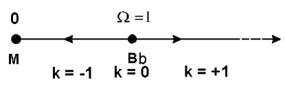
The essential point is that except for the spatially flat case
| (2) |
Observations show that
| (3) |
The flatness problem involves the explanation of (3) given (2). The problem can be viewed in two ways. First, one can take the view that there is a tuning problem in the sense that at early times must be finely tuned to peebles . However, this argument is not entirely convincing since all standard models necessarily start with exactly . More convincing is the view that except for the spatially flat case the probability that is strongly dependent on the time of observation ellis2 and so there is an epoch problem: why should (3) hold?
In this letter we point out that if then there exist standard models for which throughout their entire evolution even though they are not spatially flat. Moreover, in a precise quantitative sense, we show that these models are not finely tuned. When current observations are brought to bear on the theory, they confirm that we live in just such a universe comp .
To include with dust define, in the usual way,
| (4) |
so that the Friedmann equations reduce to
| (5) |
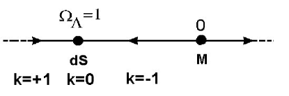
where we have written for convenience. To complement FIG. 1, which is the state space for , the state space for is shown in FIG. 2.
Evolution in the full plane was first considered by Stabell and Refsdal stabell for the case of dust (). Writing ( the standard redshift), they populated the phase plane from relations equivalent to
| (6) |
which is a restatement of the conservation law for dust (the constancy of ), and
| (7) |
which is a restatement of the constancy of . They distinguished trajectories via (half) the associated absolute horizon, . The same technique has been applied more recently and in more general situations phase .
Equivalently, from a dynamical systems point of view dynamics , we can, again using dust as an example, consider the system of differential equations
| (8) |
and
| (9) |
where and . We now recognize the critical points in FIG. 1 and FIG. 2: Bb is a repulsor, dS an attractor and M a saddle point for the full plane.
The approach used here is somewhat different. Although what now follows can be generalized further , we continue with dust as it presents an uncluttered relevant example. We observe a constant of the motion () for the system (8)-(9). The constant is given by form
| (10) |
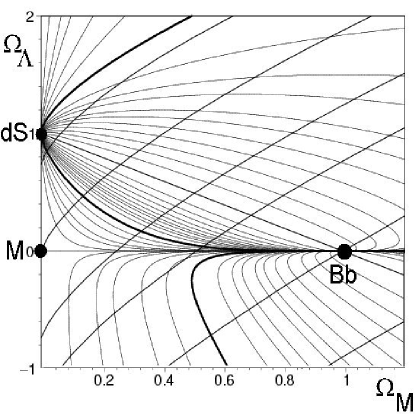
for respectively. Since for , the system can be considered solved and the Friedmann equations, in terms of observables, in effect integrated. A phase portrait with trajectories distinguished by is shown in FIG. 3.
The physical meaning of is not hard to find. In terms of the bare Friedmann equation
| (11) |
with () considered given, each value of the constant determines a unique expanding universe (). For each , if , there is a special value of that gives a static solution (the Einstein static universe or asymptotic thereto),
| (12) |
In terms of we have
| (13) |
and so is a measure of relative to the “Einstein” value static . The state spaces shown in FIG. 1 and FIG. 2 correspond to : in the first case and in the second.
As FIG. 3 makes clear, if and then
| (14) |
throughout the entire evolution of the associated universe if where is a matter of choice but of the order . In any event, it is clear that need not be finely tuned to produce (14) zero .
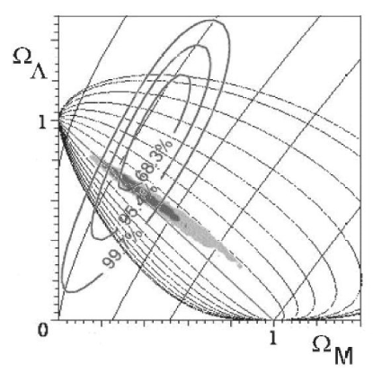
Fortunate we are to live in an era of unprecedented advances in observational cosmology. We now bring some of theses observations to bear on the foregoing discussion. The Wilkinson Microwave Anisotropy Probe (WMAP) has enabled accurate testing of cosmological models based on anisotropies of the background radiation wmap . Independently, the recent Hubble Space Telescope (HST) type Ia supernova observations Riess not only confirm earlier reports that we live in an accelerating universe Riess98 Perlmutter , but also explicitly sample the transition from deceleration to acceleration. A comparison of these results in a partial phase plane is shown in FIG. 4 current . Clearly the (WMAP) results, and to a somewhat lesser extent the (HST) results furtherhst , support the view that we live in “large” universe for which (14) has held throughout its entire evolution.
We have argued that there are an infinity of standard non-flat FLRW dust models for which throughout their entire evolution as long as . Further, we have shown that the WMAP observations confirm that we live in just such a universe. The idea can be generalized in a straightforward way to more sophisticated multi-component models wherein ( for all species but not ) from Bb to dS within a phase portrait hyper-tube about (see further for a two-component model). Note, however, that the dust model examined here is an excellent approximation now and the model relevant to a comparison with current observations. With there is no tuning or epoch problem and so no flatness problem in the traditional sense. However, our presence in this hyper-tube is presumably favored and an explanation of this probability about the trajectory in a sense presents a refinement of the classical flatness problem.
Since the analysis here has been based on the classical notion of , it is appropriate to conclude with a query as to whether or not this analysis is stable under perturbations in the definition of itself (that is “dark energy” as opposed to the classical notion of ). Since can be introduced by way of a component where , consider unspecified (but ). It can then be shown that the analysis given here generalizes in a straightforward way wcalc and that for perturbations about the phase portrait given in FIG. 3 is stable, but the state space for shown in FIG. 2 is not state2pert . This latter point in no way alters the fact that there remain an infinity of non-flat FLRW models for which throughout their entire evolution as long as .
Acknowledgements.
It is a pleasure to thank Phillip Helbig, James Overduin, Sjur Refsdal and Rolf Stabell for their comments. This work was supported by a grant from the Natural Sciences and Engineering Research Council of Canada.References
- (1) Electronic Address: lake@astro.queensu.ca
- (2) See, for example, A. H. Guth, Physics Reports 333-334, 555 (2000). Note that the argument given there is claimed to hold for , but as the argument given here shows, it does not.
- (3) For the Friedmann-Lemaître-Robertson-Walker (FLRW) models we use the following notation: is the (dimensionless) scale factor and the proper time of comoving streamlines. , , is the spatial curvature (in units of ), is the energy density and the isotropic pressure. is the (fixed) cosmological constant and 0 signifies current values. Detailed background notes and more detailed diagrams are available from http://grtensor.org/Robertson/
- (4) See, for example, J. Wainwright and G. F. R. Ellis, Dynamical Systems in Cosmology (Cambridge University Press, Cambridge 1997).
- (5) See R. H. Dicke and P. J. E. Peebles “The big bang cosmology-enigmas and nostrums” in General Relativity An Einstein Centenary Survey, Edited by S. W. Hawking and W. Israel (Cambridge University Press, Cambridge 1979). The argument is a standard one in current cosmology texts. See, for example, J. A. Peacock, Cosmological Physics, (Cambridge University Press, Cambridge 1999).
- (6) See, for example, M. S. Madsen and G. F. R. Ellis, Mon. Not. R. astr. Soc 234, 67 (1988).
- (7) The argument given here is distinct from but complementary to R. J. Adler and J. M. Overduin “The Nearly Flat Universe” arXiv:gr-qc/0501061 , A. D. Chernin “Eliminating the ‘flatness problem’ with the use of Type Ia supernova data” arXiv:astro-ph/0112158 and A. D. Chernin, New Astronomy 8, 79 (2003).
- (8) There are precisely six empty Robertson-Walker metrics: de Sitter space, which can be given in three forms (); Minkowski space, which can be given in two forms (); and anti de Sitter space, which can be given only in the form . All but the flat form of Minkowski space are shown in FIG. 2, the flat form being sent to infinity via the definition (4).
- (9) R. Stabell and S. Refsdal, Mon. Not. R. astr. Soc 132, 379 (1966). In this pioneering work the authors construct the phase portrait in the plane (in currently popular notation: , ).
- (10) J. Ehlers and W. Rindler, Mon. Not. R. astr. Soc 238, 503 (1989) consider non-interacting dust and radiation and shown phase portraits (qualitatively) but do not distinguish the trajectories quantitatively. M. S. Madsen, J. P. Mimoso, J. A. Butcher and G. F. R. Ellis, Phys. Rev. D 46, 1399 (1992) consider a number of cases with particular reference to an inflationary phase of the early universe. Again the phase portraits relevant to this discussion (their figures 10 and 11) do not distinguish the trajectories quantitatively. J. Overduin and W. Priester, Naturwissenschaften 88, 229 (2001) show phase portraits distinguished by (), a distinction which, though correct, is of no use for the present discussion.
- (11) A standard reference is ellis1 . For a recent pedagogical study see J-P. Uzan and R. Lehoucq, Eur. J. Phys. 22, 371 (2001).
- (12) A more detailed description involves a three dimensional phase portrait based on a model of non-interacting matter and radiation. This presents a phase tube of models about for which (14) (including radiation) holds. See K. Lake and S. Guha (in preparation).
- (13) The form in which (10) is given here is motivated by the fact that the only trajectory usually seen in texts and the current literature (excepting stabell - dynamics ) is as this distinguishes (for and ) ever expanding universes from those that recollapse and those with a big bang from those without. The approach used here was apparently first used by J. P. Leahy, see http://www.jb.man.ac.uk/jpl/Fdetails/
-
(14)
These loci are calculated in the usual way from
See also R. C. Thomas and R. Kantowski, Phys. Rev. D 62, 103507 (2000) arXiv:astro-ph/0003463 - (15) The constant has this physical interpretation only for and but we make use of the same constant of motion for and, in FIG. 3, also for .
-
(16)
The argument necessarily involves “large” values of
and so one might argue that the flatness issue might be solved
with for sufficiently large . Such an argument will
never remove the epoch problem because Bb is a repulsor.
The argument also involves “large” values of as is
evident from the familiar relation (for )
This explains, in elementary terms, why the universe looks “almost flat”. - (17) D. N. Spergel et al., Ap. J. Suppl. 148, 175 (2003) arXiv:astro-ph/0302209
- (18) A. G. Riess et al., Ap. J. 607, 665 (2004) arXiv:astro-ph/0402512
- (19) A. G. Riess et al., A. J. 116, 1009 (1998) arXiv:astro-ph/9805201
- (20) S. Perlmutter et al., Ap. J. 517, 565 (1999) arXiv:astro-ph/9812133
- (21) The observations of course involve the current values (). Our position in the diagram corresponds to the intersection of the “correct” value of with the correct trajectory determined uniquely by modulo .
- (22) In this regard we note that the (HST) results are certainly open to further interpretation. See, for example, J.-M. Virey, A. Ealet, C. Tao, A. Tilquin, A. Bonissent, D. Fouchez and P. Taxil, Phys. Rev. D 70, 121301(R) (2004) arXiv:astro-ph/0407452
-
(23)
Introducing the (non-interacting) species () with the dust and with no concern here for
the classical energy conditions, we have the constant and so define to replace . It follows
that equations (6), (7), (8)
and (9) are replaced by
and
respectively. More importantly, (10) generalizes to
for respectively. Now where
The stability of the phase portrait under perturbations on now follows directly. -
(24)
The instability of the state space for
, and therefore the attractor for the full phase
plane, is not difficult to see. With the
Friedmann equation is
where and here we take . This equation is unstable wrt in the sense that the qualitative behaviour of the solutions changes with . Whereas we obtain the familiar exponential solution of de Sitter space for , for we obtain
where is a constant. The associated spacetimes are singular at ( for example, the Ricci scalar diverges like ). For expanding solutions, with (), . The universe is asymptotically past flat but ends in a “Big Rip” (bR) at . (See R. C. Caldwell, M. Kamionkowski and N. N. Weinberg, Phys. Rev. Lett. 91, 071301 arXiv:astro-ph/0302506 .) We replace dS by bR in the associated phase plane and observe that all standard universes end at bR. The inclusion of a classical does not change this. For expanding solutions with () . The universe starts at a big bang but is future asymptotically flat. In this case the inclusion of a classical reverts the attractor to dS. It can be shown that these conclusions are unchanged if . Whereas it is clear that observations can never prove that (but they can prove ), it is also clear that observations also can never determine the asymptotic future state of the universe.