Joint cosmological parameters forecast from CFHTLS-cosmic shear and CMB data

We present a prospective analysis of a combined cosmic shear and cosmic microwave background data set, focusing on a Canada France Hawaii Telescope Legacy Survey (CFHTLS) type lensing survey and the current WMAP-1 year and CBI data. We investigate the parameter degeneracies and error estimates of a seven parameters model, for the lensing alone as well as for the combined experiments. The analysis is performed using a Monte Carlo Markov Chain calculation, allowing for a more realistic estimate of errors and degeneracies than a Fisher matrix approach. After a detailed discussion of the relevant statistical techniques, the set of the most relevant 2 and 3-dimensional lensing contours are given. It is shown that the combined cosmic shear and CMB is particularly efficient to break some parameter degeneracies. The principal components directions are computed and it is found that the most orthogonal contours between the two experiments are for the parameter pairs $(\Omega_{m},\sigma_{8})$, $(h,n_{s})$ and $(n_{s},\alpha_{s})$, where $n_{s}$ and $\alpha_{s}$ are the slope of the primordial mass power spectrum and the running spectral index respectively. It is shown that an improvement of a factor $2$ is expected on the running spectral index from the combined data sets. Forecasts for error improvements from a wide field space telescope lensing survey are also given.

1 Introduction

The Canada-France-Hawaii Telescope Legacy Survey (CFHTLS) is a long term wide field imaging project that started in early 2003 and should be completed by 2008. The French and Canadian astronomical communities will spend about 500 CFHT nights to carry out imaging surveys with the new Megaprime/Megacam instrument recently mounted at the CFHT prime focus. About 160 nights will focus on the ”CFHTLS-Wide” survey that will cover 170 deg², spread over 3 uncorrelated patches of $7^{o}\times 7^{o}$ each, in $u^{*},g^{\prime},r^{\prime},i^{\prime},z^{\prime}$ bands, with typical exposure times of about one hour per filter. The ”CFHTLS-Wide” survey design and observing strategy are similar to the Virmos-Descart cosmic shear survey but it will have a sky coverage 20 times larger. It is widely seen as a typical second generation cosmic shear survey.

The exploration of weak gravitational distortion produced by the large scale structures of the universe over field of views as large as ”CFHTLS-Wide” has an enormous potential for cosmology. Past experiences based on first generations cosmic shear surveys (see for example reviews in Van Waerbeke & Mellier (2003); Réfrégier (2003)) have demonstrated they can constrain the dark matter properties ($\sigma_{8}$, $\Omega_{m}$ and the shape of the dark matter power spectrum) from a careful investigation of the ellipticity induced by weak gravitational shear on distant galaxies. For example, the most recent cosmic shear results from the Virmos-Descart survey (Van Waerbeke et al. (2004)) lead to the conservative limits $\sigma_{8}=0.85\pm 0.15$ (99% C.L.) and $\Omega_{m}=0.3\pm 0.15$ (99% C.L.), which means an expected accuracy of $\approx$1-3% can be expected with the ”CFHTLS-Wide” for the same set of cosmological parameters. The CFHTLS-Wide will also explore a broader wavenumber range (10⁵-10²) than Virmos-Descart and will extend to linear scale, that will considerably ease cosmological interpretation of weak lensing data. The second generation surveys will therefore permit to investigate more thoroughly different cosmological models, taking into account a broad range of cosmological parameters. For instance, the CFHTLS as a probe dark energy evolution was stressed out by Benabed & van Waerbeke (2003).

The full scientific outcome of the cosmic shear data from the ”CFHTLS-Wide” will only be complete with a joint analysis with other data sets, like Type Ia Supernovae, galaxy redshift surveys, Lyman-alpha forest, or CMB observations. Contaldi et al. (2003) have used the Red Cluster Sequence (RCS) cosmic shear survey together with the CMB data. It was shown that the $\Omega_{m},\sigma_{8}$ degeneracies for lensing and CMB are nearly orthogonal, which makes this set of parameters particularly relevant for such combined analysis (Van Waerbeke et al. (2002)). The search for orthogonal parameter degeneracies between different observations is one of the most important aspects of parameters measurements.

 Ishak et al. (2003) recently argued that joint CMB-cosmic shear surveys provide an optimal data set to explore the amplitude of the running spectral index and probe inflation models. They used a Fisher-Matrix analysis on WMAP+ACBAR+CBI and a ”reference survey”. Their simulated survey covers about 400 deg² with a depth corresponding to a galaxy number density of lensed sources of about 60 arc-min^-2, and they restricted their analysis to 3000$>l>$20. They found that several parameters can be significantly improved (like $\sigma_{8}$, $\Omega_{m}h^{2}$, $\Omega_{\Lambda}$) and in particular that both the spectral index $n_{s}$ and the running spectral index $\alpha_{s}$ errors are reduced by a factor of 2. Their encouraging results show that joint CMB and weak lensing data may provide interesting insights on inflation models. Here, we investigate the 2-dimensional structure of the parameter degeneracies between lensing and CMB data sets, and look for the expectation with a ”CFHTLS-Wide”-like survey design.

To explore the smaller scales probed by the ”CFHTLS-Wide”, which will provide cosmic shear information down to 20 arc-seconds, it is preferable to avoid prior assumptions regarding the Gaussian nature of the underlying distribution, and to discard a Fisher matrix analysis. We used in this work the so-called Markov Chain Monte Carlo (MCMC) method. The MCMC computing time linearly scales with the number of parameters and eases the exploration of a large sample of parameters and a broad range of values for each. Contaldi et al. (2003) already used this approach with the RCS survey to map the $\Omega_{m},\sigma_{8}$ parameter space, but marginalised over a small set of cosmological parameters. The goal of this present work is to map the parameter space that describes cosmological models in order to extract series of parameter combinations that would minimise intersections of CMB and cosmic shear degeneracy tracks. Compared to the Fisher-Matrix approach which produces ellipses only, MCMC provides more details of the parameter space and eventually a more realistic estimate of error improvements of the joint analyses.

The paper is organised as follows: Section 2 introduces the gravitational lensing and defines the cosmic shear fiducial data used and the parameter space investigated. Section 3 gives the details of our MCMC calculations, limitations and convergence criteria. Section 4 shows the MCMC results from the cosmic shear alone, assuming a lensing survey similar to the CFHTLS. In Section 5 we present the results of the parameter degeneracies analysis on the combined cosmic shear and cosmic microwave background observations. The assumptions made and the results obtained are discussed in section 6 and we conclude in section 7.

2 Cosmic shear and Cosmological parameters

Propagation of galaxy light beams across large scale mass inhomogeneities produces distorted and (de)magnified galaxy images (for reviews see Mellier (1999); Bartelmann & Schneider (2001); Réfrégier (2003); Van Waerbeke & Mellier (2003)). The gravitational lensing magnification and shear are described by the amplification matrix which involves second order derivatives of the projected gravitational potential $\varphi$ : the shear, $\gamma$, and the convergence, $\kappa$,

$$\kappa={1\over 2}\left(\varphi_{,11}+\varphi_{,22}\right)\ ;\ \ \gamma_{1}={1\over 2}\left(\varphi_{,11}-\varphi_{,22}\right)\ ;\ \ \gamma_{2}=\varphi_{,12}.$$ (1)

The cosmic shear may be derived from the ellipticity of the galaxies. In the weak lensing approximation, the observed ellipticity of a galaxy is related to its intrinsic ellipticity and to the shear by,

$$\epsilon_{i}=\epsilon_{is}+\gamma\ ,$$ (2)

where $\epsilon_{i}=(\epsilon_{xi},\epsilon_{yi})$ and $\gamma=(\gamma_{1},\gamma_{2})$. Several correlation functions and 2-point statistics of the shear may be defined. In this work we will use the shear variance in a top-hat window of radius $\theta$ (Eq. (7)), although all 2-points statistics are equivalent and provide similar results (they are all linear combinations of the others). Let us now relate this quantity to cosmology.

We parameterize cosmological models with a set of 13 parameters, $(\omega_{b},\omega_{c},\Omega_{v},f_{\nu},h;\sigma_{8},n_{s},\alpha_{s},r,n_{t};\tau;w;z_{s})$. Each model defines a point in the high-dimensional space where a value of the likelihood of the model with respect to the data may be calculated. We use the CAMB software (Lewis et al. (2000)) to compute the dark matter power spectrum and transfer function. The parameters are defined as follow:

• $(A_{s},n_{s},\alpha_{s})$ - parameterize the primordial scalar power spectrum:

  $$P(k)=A_{s}{\left(k\over{k_{0s}}\right)}^{n_{s}(k_{0s})-1+{1\over 2}\alpha_{s}\ln({k\over k_{0s}})},$$ (3)

  which is normalized with $A_{s}=P(k=0.05h{\rm Mpc}^{-1})$ and has a scale-dependent tilt.

• $(A_{s},r,n_{t})$ - parameterize the primordial tensor power spectrum:

  $$P(k)=rA_{s}{\left(k\over{k_{0t}}\right)}^{n_{t}},$$ (4)

  with $k_{0t}=0.002h{\rm Mpc}^{-1}$.

• $(\omega_{b},\omega_{c},\Omega_{v},f_{\nu})$ - the matter budget consisting of baryons, cold dark matter, dark energy and neutrinos, with $\omega_{b}=\Omega_{b}\,h^{2}$, $\omega_{c}=\Omega_{c}\,h^{2}$.

• $(h)$ - the hubble parameter. The spatial curvature is not a free parameter : $\Omega_{k}=1-\Omega_{v}-(\omega_{c}+\omega_{b})/h^{2}.$

• $(w)$ - dark energy equation of state parameter.

• $(\tau)$ - reionization optical depth.

• $(\sigma_{8})$ - Once the 3-dimensional power spectrum of the density fluctuations is derived, it is renormalized according to the model value of $\sigma_{8}$, losing the memory of the original value of $A_{s}$.

The non-linear evolution of the power spectrum is then evaluated using the halofit prescription of Smith et al. (2003). The power spectrum of the gravitational convergence is derived by integrating the dark matter power spectrum along the line-of-sight from the observer up to the radial coordinate of the horizon $\chi_{H}$:

$$P_{\kappa}(k)={9\over 4}\Omega_{m}^{2}\int_{0}^{\chi_{H}}{\rm d}\chi{g^{2}(\chi)\over a^{2}(\chi)}P_{3D}\left({k\over f_{K}(\chi)};\chi\right)\ ,$$ (5)

where $k$ is the 2-dimensional wave vector perpendicular to the line-of-sight. $f_{K}(\chi)$ is the comoving angular diameter distance to a coordinate $\chi$, and $g(\chi)$ is given by

$$g(\chi)=\int_{\chi}^{\chi_{H}}{\rm d}\chi^{\prime}p(\chi^{\prime}){f_{K}(\chi^{\prime}-\chi)\over f_{K}(\chi^{\prime})},$$ (6)

where $p(\chi(z))$ is the source redshift distribution, which depends on the last item in our cosmological parameters set:

• $(z_{s})$ - the redshift of the sources.

For simplicity, we assume that all the sources are at a single redshift, $z_{s}$, but the generalisation to a broad redshift distribution is straightforward.

From the power spectrum of the gravitational convergence, the top-hat shear variance inside a circle of radius $\theta$ can be computed:

$$\langle\gamma^{2}(\theta)\rangle={2\over\pi\theta^{2}}\int_{0}^{\infty}\leavevmode\nobreak\ {{\rm d}k\over k}P_{\kappa}(k)[J_{1}(k\theta)]^{2}.$$ (7)

Table 1: Cosmic shear : fiducial cosmological model.

$\omega_{b}=0.022$	$\omega_{c}=0.114$	$\Omega_{v}=0.73$
$f_{\nu}=0$	$\Omega_{k}=0$	$h=0.71$
$n_{s}(k_{0s})=0.93$	$\alpha_{s}(k_{0s})=-0.04$	$r=0$
$w=-1$	$\tau=0.17$
$\sigma_{8}=0.9$	$z_{x}=0.8$

For each cosmological model generated by the Monte Carlo simulation described in the next section, $\langle\gamma^{2}(\theta)\rangle$ is computed and compared to a fiducial data model, $\langle\gamma^{2}_{\;\rm data}(\theta)\rangle$ that corresponds to the fiducial cosmological model of Table 1. This is taken to be the best fit $\Lambda CDM$, flat, no neutrinos, no gravitational waves, running spectral index model, derived from the first year WMAP data (Spergel et al. (2003)). The sources are placed at $z_{s}=0.8$. The likelihood of each model is given by

$$-2\,{\cal L}=\left(\langle\gamma^{2}\rangle_{i}-\langle\gamma^{2}_{\;\rm data}\rangle_{i}\right)C_{\rm data\,ij}^{-1}\left(\langle\gamma^{2}\rangle_{\,j}-\langle\gamma^{2}_{\;\rm data}\rangle_{j}\right),$$ (8)

where $C_{\rm data\,ij}$ is the covariance matrix

$$C_{\rm data\,ij}=\langle\left(\gamma_{i}^{2}-\gamma_{{\rm data}\leavevmode\nobreak\ i}^{2}\right)\left(\gamma_{j}^{2}-\gamma_{{\rm data}\leavevmode\nobreak\ j}^{2}\right)\rangle.$$ (9)

The covariance matrix of a shear dispersion distribution is analytically derived in Schneider et al. (2002). The shear dispersion at a given angular scale $\theta$ may be expressed as an integral of the two-point correlation of galaxy ellipticities, $\xi_{+}$, estimated in bins of angular separation $\Delta\vartheta$ at the center position $\vartheta_{i}$, evaluated with a window function $S_{+}(\vartheta_{i}/\theta)$. The covariance of the shear dispersion involves the four-point ellipticities correlations. Eq. (2) shows they depend on the intrinsic ellipticity correlations, and therefore on the intrinsic ellipticity dispersion $\sigma_{\epsilon}$, and on the shear correlations for each model. The shear field is assumed to be Gaussian, so that the 4-point function can be factorised as a sum over products of 2-point functions. It is assumed that the covariance matrix depends solely on the fiducial cosmological model. Assuming a connected single field of solid angle $A$ and a mean density $n_{g}$ of source galaxies with an intrinsic ellipticity dispersion of $\sigma_{\epsilon}$, the ensemble average of the covariance matrix, ${\rm Cov}(\mathcal{S};\theta_{1},\theta_{2})$ of the estimator $\mathcal{S}$ of $\langle\gamma^{2}(\theta)\rangle$ is,

$${\rm Cov}(\mathcal{S})={{\sigma^{4}_{\epsilon}}\over{2\pi\,A\,n_{g}^{2}}}\int_{0}^{2\rm min(\theta_{1},\theta_{2})}{d\vartheta\,\vartheta\over\theta_{1}^{2}\theta_{2}^{2}}\left[S_{+}\left({\vartheta\over\theta_{1}}\right)S_{+}\left({\vartheta\over\theta_{2}}\right)\right]+$$

(10)

$$\int_{0}^{2\theta_{1}}{d\vartheta_{1}\,\vartheta_{1}\over\theta_{1}^{2}}\int_{0}^{2\theta_{2}}{d\vartheta_{2}\,\vartheta_{2}\over\theta_{2}^{2}}\left[S_{+}\left({\vartheta_{1}\over\theta_{1}}\right)S_{+}\left({\vartheta_{2}\over\theta_{2}}\right)C^{\prime}_{++}(\vartheta_{1},\vartheta_{2})\right].$$

Eq. (2) is the Eq. (42) in Schneider et al. (2002) transposed for the dispersion $\langle\gamma^{2}\rangle$. The first term is a pure Poisson noise term, due to the intrinsic ellipticities of the galaxies. Its value decreases rapidly with the scale $\theta$. The second term is determined by $C^{\prime}_{++}(\vartheta_{1},\vartheta_{2})$, the shear correlations dependent part of $C_{++}$ (the covariance matrix of $\xi_{+}$). It is computed using equations (32) and (34) of Schneider et al. (2002) with the the shear correlation function computed from the convergence power spectrum at the fiducial model as,

$$\xi_{\pm}(\theta)={1\over 2\pi}\int_{0}^{\infty}{\rm d}k\,kP_{\kappa}(k)J_{0,4}(k\theta).$$ (11)

We do not include extra sources of errors, in particular we assume that galaxy shape measurement and PSF anisotropy corrections are free of systematics.

Figure 1: Shear variance as a function of scale. The bottom left plot shows the fiducial model with $3\,\sigma$ error bars. In the other 8 plots, we change the labelled parameter by a step of $+10\%$ (solid line) and $-10\%$ (dashed line), except for $\alpha_{s}$ where the step is $\pm 100\%$. In each case, the other 7 labelled parameters are kept constant. Flatness is not imposed.

Table 2 summarizes the survey properties.

Table 2: Cosmic shear : survey specifications.

Size of the survey:	A=$170\,{\rm deg}^{2}$
Density of galaxies:	$n_{g}=20\,{\rm arcmin}^{-2}$
Intrinsic ellipticity dispersion:	$\sigma_{\epsilon}=0.4$
Scales probed:	$0.6\,^{\prime}<\theta<2\deg$
	$90<l<18000$

These are based on real observations; the values for $\sigma_{\epsilon}$ and $n_{g}$ (the effective density, once galaxy selection is done) are found in cosmic shear surveys (Van Waerbeke et al. (2002)) and the field size is the total size of the CFHT Legacy Survey. To choose the upper limit on the angular scale, we notice, from Eq. (2), that the computation of the covariance of the shear dispersion at a scale $\theta$ involves an integration up to $2\,\theta$. Furthermore, the integrations involved in the computation of $C^{\prime}_{++}$ need an extra factor of $\sqrt{2}$. We define $\theta_{max}$ to be such that $2\,\sqrt{2}\,\theta_{max}$ corresponds to the largest wavelength that can fit in a field of the survey area. Given that the fields of the CFHTLS-Wide survey have an approximate size of $7\degr\times 7\degr$, we find $\theta_{max}$ to be around $2\,\degr$. The lower limit on the scale probes the deep non-linear regime.

The solid line in the bottom left plot of Fig. 1 shows the shear variance of the fiducial model (Table 1) as function of angular scale, along with $3\sigma$ error bars computed from Eq. (2) at 20 angular scale points ranging from $0.6\,{\rm arcmin}$ to $2\degr$. The error bars are smaller at intermediate scales, slightly larger at the smallest scales, where they are determined by statistical noise, and are noticeably bigger at the largest scales, which are cosmic variance dominated. They are slightly optimistic at small angular scales, due to the Gaussianity assumption, made in the derivation of the covariance, lacking the non-linear enhancement of the signal The dashed line shows the shear variance without the non-linear corrections. Both lines become well separated below $10{\rm\leavevmode\nobreak\ arcmin}$. The other panels on Fig. 1 illustrate the cosmic shear sensitivity to different cosmological parameters. From this figure, it is clear that cosmic shear is more sensitive to $\Omega_{m}$, $\sigma_{8}$ and the source redshift, with the cosmic shear signal increasing with the increase of these parameters. It also shows that the dependence on $n_{s}$ is a stronger function of scale than for the other parameters. This is in agreement with theoretical expectations derived from linear perturbation theory (Bernardeau et al. (1997)):

$$\langle\gamma^{2}(\theta)\rangle^{1/2}\propto\sigma_{8}\,\Omega_{m}^{0.75}\,z_{s}^{0.8}\,\left({\theta\over 1^{\prime}}\right)^{-(n_{s}+2)/2}.$$ (12)

The measurement of the signal down to small (non-linear) scales introduces additional parameter sensitivity with some degeneracies broken, like for instance the parameter pair ($\Omega_{m}$, $\sigma_{8}$), as shown in Jain & Seljak (1997). This gain in sensibility is also noticeable in the $\alpha_{s}$ case.

3 Markov chain Monte Carlo

3.1 General considerations

The probability distribution function (PDF) of an $m$-dimensional vector parameter $\bf{p}$ given the $n$-dimensional vector data $\bf{x}(\bf{p}_{0})$ (the posterior PDF $P(\bf{p}|\bf{x})$), can be calculated using Bayes theorem from the prior PDF $P(\bf{p})$ and the conditional PDF of the data given the parameter vector (the likelihood $L(\bf{x}|\bf{p})$) :

$$P(\bf{p}|\bf{x})={{P(\bf{p})L(\bf{x}|\bf{p})}\over{\int{P(\bf{p})L(\bf{x}|\bf{p})d\bf{p}}}}.$$ (13)

Its analytical computation would involve high-dimensional integrations, not only to compute the normalisation (also called the evidence or the marginalised posterior) but also to extract information from the posterior, such as the determination of means or marginalised lower dimensional distributions. Thus, Eq. (13) is analytically solved only for special cases: For Gaussian PDFs, with mean given by $\bf{p}_{0}$, we see from Eq. (13) that the posterior inverse covariance matrix is $C^{-1}_{ij}=F_{ij}+F^{prior}_{ij}$, where $F$ is the Fisher information matrix,

$$F_{ij}=\left<{{\partial^{2}\cal L}\over{\partial p_{i}\partial p_{j}}}\right>_{\bf{x}}\equiv\left({{\partial^{2}\cal L}\over{\partial p_{i}\partial p_{j}}}\right)_{\bf{p}=\bf{p}_{0}}.$$ (14)

In general, for non-gaussian PDFs, this Fisher matrix method still gives valuable information, since we can always Taylor-expand $\cal L=-\ln$ $L$ around the point of maximum likelihood, $\bf{p}=\bf{p}_{0}$, obtaining, to quadratic order,

$$\Delta\cal L(\bf{p})=(\bf{p}-\bf{p}_{0})^{t}F(\bf{p}-\bf{p}_{0}),$$ (15)

and use the Fisher matrix as a linear approximation to the inverse covariance matrix. Being a covariance matrix of a real physical problem, $F^{-1}$ must be positive-definite. Therefore an hypersurface of constant $\Delta\cal L(\bf{p})$, as defined by Eq. (15), is an hyperellipse which will be an approximation of a certain $\sigma$ volume of the posterior. The one-dimensional parameters marginalised errors, i.e., integrated over the other components of the parameters vector, are given by $\Delta p_{i}(1\sigma)=(F^{-1}_{ii})^{1/2}$. From Eq. (15) it is clear that $\Delta p_{i}(1\sigma)=(F_{ii})^{-1/2}$ is the error on $p_{i}$ when all parameters but $p_{i}$ are fixed at $\bf{p}_{0}$. Note that, since the Fisher matrix is exactly the quantity involved in the Rao-Cramér inequality, the errors computed from the Fisher matrix approximation are always lower limits of the true ones.

In practice, in order to obtain a more precise result, the problem is usually solved by computing the posterior at optimized sample points that pave the parameter space. The traditional approach uses a regular grid. This is a computer-intensive procedure with computation time rising exponentially with the space dimension, which limits the number of parameters that can be explored. Markov chain Monte Carlo sampling (Gilks et al. (1996)) overcomes this limitation.

The use of the MCMC technique in cosmological parameters estimation was first implemented in Christensen et al. (2001), following the proposal of Christensen & Meyer (2001). Current tools like CosmoMC (Lewis & Bridle (2002)) no longer evaluate the likelihood at fixed points but at selected positions of a Markov chain. Each chain point, $p_{i+1}$, is derived from the previous chain point, $p_{i}$, in such a way that the transition probability from $p_{i}$ to $p_{i+1}$ times the posterior PDF of $p_{i}$, equals the product of the transition probability from $p_{i+1}$ to $p_{i}$ by the posterior PDF of $p_{i+1}$. Thus, after a relaxation time, the chain reaches the equilibrium and constitutes a sample of the posterior. A clear advantage of this is that statistical properties of the distribution, like the mean of a parameter or a marginalised confidence interval, can be directly derived from discreet sample points, without need to use the computed values of the likelihood. Different priors may also be introduced adapting the weighting scheme defined by the sample, without need to build a new chain.

The computing time is determined by the number of points needed to converge to the equilibrium distribution. If the chain is built in an efficient way, CPU time scales linearly with the dimension of the parameter space. Computing time may be reduced by finding an analytical expression for the posterior. For example, the Markov chain data is used to fit the log-likelihood with a polynomial in Sandvik et al. (2003).

3.2 MCMC Analysis

The MCMC code we developed is based on the Metropolis-Hastings algorithm (Metropolis et al. (1953) and Hastings (1970)), like CosmoMC (Lewis & Bridle (2002)), Cog (Slozar & Hobson (2003)) or the AnalyzeThis (Doran & Müller (2003)) public software.

3.2.1 Chain progression rules

We start several chains at different initial positions chosen randomly inside the limited part of the 7-dimensional parameter space we aim to explore (Table 3).

Table 3: Parameters and exploration range investigated by the MCMC chain : The upper part of the table shows the 7 parameters used in the initial proposal density, along with their exploration range. The bottom part shows extra imposed limits to the MCMC exploration. Other independent cosmological parameters are kept constant at their fiducial values.

$\omega_{b}$		0.01	0.04
$\omega_{c}$		0.01	0.3
$h$		0.4	1.0
$n_{s}$		0.5	1.4
$\Omega_{v}$		0.3	0.9
$\alpha_{s}$		-0.2	0.2
$\sigma_{8}$		0.6	1.2
$\Omega_{K}$		-0.1	0.1
$Age$	(Gyr)	10	20
$\Omega_{c}$	$<$	3$\Omega_{b}$

The next point is proposed using a proposal PDF, $q(p_{i+1}|p_{i})$ and the unnormalised posteriors of both points are compared to decide if the new point is acceptable. The PDF acceptance rule we use for the next step point $p_{i+1}$ is defined by

$$\alpha(p_{i+1}|p_{i})=min\left\{{{p(p_{i+1})L(x|p_{i+1})q(p_{i}|p_{i+1})}\over{p(p_{i})L(x|p_{i})q(p_{i+1}|p_{i})}},1\right\}.$$ (16)

$\alpha$ is compared to a random number $u$ generated from a uniform distribution between 0 and 1. If $\alpha>u$, then the new $p_{i+1}$ is accepted; otherwise it is rejected and we keep the point $p_{i+1}=p_{i}$. Since both the proposal and the acceptance densities only depend on the current element of the chain and not on its previous history, the resulting sample will be a Markov chain. It is worth noticing that the ratio in this definition makes the normalisation of the posterior PDF unnecessary. Furthermore, the presence of the proposal PDF in Eq. (16), ensures that $p(p)L(x|p)$ is the equilibrium function, even in the case of a non-symmetrical $q$, i.e. when the probability of proposing $p$ from $p^{\prime}$ is different from that of proposing $p^{\prime}$ from $p$.

The result is independent of the proposal density, $q$. We use as $q$, at the beginning of the chain, a 2-dimensional Gaussian distribution centered at the current chain element. Hence, only 2 of the 7 parameters (randomly chosen) change at each step. The covariance matrix of $q$ is chosen to be of the order of the expected, squared, $1\sigma$ error bars. The $1\sigma$ error value is used as the step definition criterion and guarantees the step amplitude has an adequate size. Would it be too small, the chain would move too slowly and could never leave the vicinity of the best fit. This situation is known as poor mixing and leads to underestimated confidence limits. In contrast, if the proposed steps are too large, the acceptance rate will be too small and once again the chain will move slowly.

In order to have an adequate initial proposal density we derived approximate $1\sigma$ errors from a Fisher matrix computation. Applying Eq. (14) to Eq. (8) leads to (Tegmark et al. (1997)),

$$F_{ij}=\sum_{\alpha=1}^{n}\,\sum_{\beta=1}^{n}C^{-1}_{\alpha\beta}\,\left({{\partial\langle\gamma^{2}\rangle_{\alpha}}\over{\partial p_{i}}}{{\partial\langle\gamma^{2}\rangle_{\beta}}\over{\partial p_{j}}}\right),$$ (17)

where the derivatives of the shear variance are evaluated at the fiducial model. To numerically evaluate these derivatives, we compute the shear variances at points $p_{i}^{fid}\pm\,\Delta\,p_{i}$, with the deltas ranging from $0.1\%$ to $10\%$ depending on the sensitivity of the shear statistic to each cosmological parameter, $p_{i}$. However, computing and sampling errors, coming mainly from the near cancellation of certain combinations of derivatives, as was pointed out by Einsentein et al. (1998), generate small fluctuations in the Fisher matrix coefficients that are amplified by matrix inversion when the covariance matrix is derived from the Fisher matrix. For this reason, we did not use the inverse Fisher matrix as the covariance matrix of the initial proposal density, but used instead a diagonal covariance matrix whose ratios between coefficients are equal to the ratios between the diagonal coefficients of the inverse Fisher matrix. It is worth noticing that one way to obtain a not so nearly singular Fisher matrix is to include the derivatives of the data covariance matrix in the derivation of the Fisher matrix formula (Eq. (17)).

In order to better explore the directions of degeneracy and consequently speed up the convergence, a non-diagonal proposal covariance matrix is needed. Hence, after $1000$ steps, the covariance matrix of the chain in progress is computed. From it, a new set of 7 parameters, aligned with the eigenvectors of the evaluated correlation matrix, is defined. From that step on, the new sample points are built from a combination of 2 eigenvector directions, randomly chosen at each step. Though it defines the next direction, the step size does not necessarily needs to match the corresponding eigenvalues. In fact, after 1000 steps the covariance matrix is smaller than it will be at its converged value, so we must scale it. We update periodically the proposal covariance matrix. However, since this process computes a new sample covariance matrix, it cannot be done too frequently; otherwise the progression of the chain too much depends on the previous elements and would no longer be a Markov chain. After a few periods we freeze the proposal density and set the multiplicative correction factor to 1. The optimal scaling value depends on the number of dimensions probed (Gelman (1996)).

3.2.2 Convergence and goodness

The first elements of a chain depend on the starting point. It is only after a so called burn-in period that the chain starts sampling the target density. Although it is not possible to say with certainty that a finite sample from an MCMC algorithm is representative of the target distribution, several tests have been proposed to detect non-convergence of the chain (for a review see Cowles & Carlin (1994)). In this work, we used the Gelman and Rubin test to estimate the size of the burn-in.

Let us consider a Markov chain of a given parameter composed of $2n$ iterations. Due to the random selection process of the starting point we expect $m$ different chains to differ significantly at the beginning and to converge towards the same distribution as the number of iteration steps increases. The burn-in interval is set when the typical separation of several chain points at a given iteration is similar to the amplitude of the chain internal fluctuations. At each iteration $i$, two quantities can be computed for each parameter:

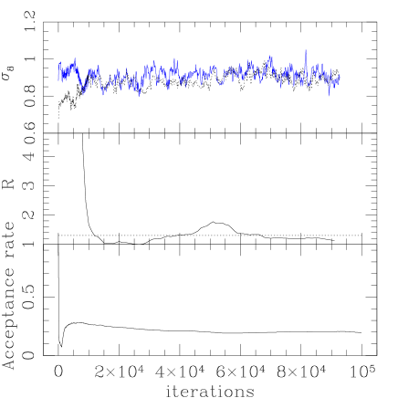
Figure 2: Monitoring a chain.The upper plot shows the successive values of $\sigma_{8}$ for two of the CFHTLS simulated chains with different starting points. In the middle plot, the Gelman and Rubin test between these 2 chains is made at several stages. This example shows that it is possible to detect an apparent convergence around the iteration step $20\times 10^{3}$. From the iteration $60\times 10^{3}$ on, $R$ started to consistently approach 1 for all parameters, leading us to choose a burn-in of $30\times 10^{3}$. The horizontal line is R=1.3. In the bottom plot, the acceptance rate of one chain is computed at each iteration $i$, using all chain elements from the first one up to $i$. In the very beginning we notice two opposite behaviors : a shear drop and a steady raise. The transition takes place at the moment the proposal density starts to follow the covariance matrix of the sample, showing the efficiency of that procedure. Afterwards, the acceptance rate drops slowly stabilizing at about $20\%$.

• The within-chain variance, $W(p)$, is the average of the $m$ variances of the parameter,

  $$W(p)={{1\over m}\sum_{j=1}^{m}\,{1\over{n-1}}\sum_{i=n}^{2n}\,(p_{i}(j)-<p>_{i}(j))^{2}}.$$ (18)

• The between-chains variance, $B(p)$, is the variance of the parameter means from the $m$ chains,

  $$B(p)={{1\over{m-1}}\sum_{j=1}^{m}\,(<p>_{i}(j)-<<p>_{i}(j)>_{j})^{2}}.$$ (19)

In the first iterations, each chain is concentrated in a different starting region, so $B$ is in most cases much larger than $W$. When the iterations increase, $W$ grows while $B$ decreases and get closer and closer to zero at convergence. Since it is not possible to explore the whole space, $W$ is always an underestimate of the within-chain variance. Hence, $B+W$ is an overestimate of the parameter variance. In the limit $i\rightarrow\infty$, both estimators approach the true variance from opposite sides. Their ratio,

$$R={1\over W}\left(B+{W\,n\over{n-1}}\right),$$ (20)

is therefore a suitable estimate to monitor the convergence.

When, after $2n$ iterations, $R$ is close to one for all the quantities of interest, i.e., for all the parameters and derived parameters we want to analyse, we assume the chain has converged. The first $n$ iterations are the burn-in period. They are discarded and the actual marginalised posterior density of a parameter is drawn by its frequency of appearance in each bin, during the iterations $n+1$ to $2n$. When after $2n$ iterations there was not enough time to explore the tails of the distribution the errors of the target distribution are underestimated. Therefore, it is useful to let the chains run for a longer period in order to get a better mixing. In the process, the value of the estimate $R$ may raise before getting smaller again. We show an example of this situation in Fig. 2, where we follow a chain evolution.

Once a chain has stopped, we must remove the residual correlation between the consecutive elements. For this reason it is recommended to thin the chain out, i.e., to keep only 1 out of $k$ consecutive elements. The most widespread method in the literature to determine the thinning factor, $k$, is the Raftery and Lewis method (RL)(Raftery & Lewis (1996)).

Figure 3: The standard deviation of $\sigma_{8}$ computed from different samples taken from the same chain by using different thinning factors is plotted against the thinning in logarithmic scale.

This method starts by constructing several chains from the converged MCMC chain, by thinning the latter with several different values. A weight may be assigned to each one of the thinned chains, according to its compatibility to an independence chain (a chain with no correlation between its consecutive elements). RL computes the weight of a chain from the ratio between its evidence and the evidence of an independence chain. The evidences are computed in the Bayesian Information Criterium (BIC) form of Schwarz (1978), which is a gaussian approximation that may be derived from the Bayes formula (Eq. (13)). It writes, $\rm{ratio}=\rm{BIC}=G^{2}-2\,{\sc log}\,n$, where $n$ is the number of elements in the chain. The $G^{2}$ statistic is a $\chi^{2}$ that measures the fit of a chain to an independence chain. To obtain $G^{2}$, one counts the number of transitions between bins of the chain, in order to get the ratio between the probability of the chain to have a certain value at a certain step $i$ for a given chain value of a previous step $i-j$, and the probability independently of the value at $i-j$. In practice, when counting the transitions, only 2 bins are assumed, i.e, a chain element becomes a 0 or a 1 as whether its parameters values are less or greater than a certain cut-off, that we choose to be the parameters $2\sigma$ values. The greatest weight is attributed to the longest chain verifying $BIC<0$. Its thinning value is the obtained $k$ factor and that chain is the best-fit to an independence chain that can be obtained by thinning the original chain.

It is worth noting that this is an application of the use of the evidence to the problem of selection between different sets. Another evidence based weighting scheme is used when combining different sets of cosmological data in Hobson et al. (2002).

There are other methods to estimate a thinning factor. In particular, Tegmark et al. (2003) obtain it by defining a more intuitive chain correlation length. Using RL, we obtained very large thinning factors for some of the MCMC chains (of order 100). However, we checked the dependence of the results on the thinning factor, by computing the parameters confidence levels using several chains, thinned from the original chain with different values of $k$ and found no appreciable difference in the results (see Fig. 3 for an example). Hence, in order not to lose so many chain elements we did not use the Raftery and Lewis method results, but a simpler criterium: for each chain we choose the thinning factor as the average multiplicity of the chain elements.

The results in the next section are computed from 4 chains with $10^{5}$ elements each, with a burn-in size of $30\times 10^{3}$ and a thinning factor of 5. The chains were merged, leading to a final sample with about 50 000 elements.

4 Cosmological parameters from CFHTLS cosmic shear statistics only

Table 4: Numerical results for the cosmic shear sample, including $1\sigma$ precision on individual parameters and a principal components analysis. I: $68\%$ confidence levels in absolute value (first line) and in percentage of the corresponding parameter fiducial value (second line). II: The 7 eigenvectors of the correlation matrix ordered by decreasing accuracy. The column named $1\sigma$, lists the dispersion of each $X$ parameter defined in Eq. (21), which is equivalent to the square root of the corresponding eigenvalue. Each line $i$ shows the coefficients $a_{ij}$ of Eq. (21), i.e., the projections of the corresponding $X_{i}$ on each of the 7 parameters $p_{j}$ labeled on the very top of the table. Naturally the derived parameter $\Omega_{m}$ is not used for the computation of the eigendirections and $\sum_{j=1}^{7}\,a_{ij}^{2}=1$. III: The 7 eigenvectors computed for mean subtracted data normalized by the means. The parameters used are $(\Omega_{b},\Omega_{m},h,n_{s},\Omega_{v},\alpha_{s},\sigma_{8})$. The column $1\sigma$, lists the dispersion of each $Y$ parameter defined in Eq. (22). The next 7 columns show the components, $b_{ij}$, of the $Y_{i}$. In the last column we show the relative contribution of the main parameter involved in each pc. IV: Each line shows the fractional error of each of the 7 parameters $(\Omega_{b},\Omega_{m},h,n_{s},\Omega_{v},\alpha_{s},\sigma_{8})$ computed using a limited number of principal components. The first line, $\#pc=1$, refers to using only the projections of $Y_{7}$. In $\#pc=2$ both $Y_{7}$ and $Y_{6}$ are used. Using all the PCS, we recover, in the last line, $100\%$ of the error values for all parameters.

I			$\omega_{b}$	$\omega_{c}$	$h$	$n_{s}$	$\Omega_{v}$	$\alpha_{s}$	$\sigma_{8}$	$\Omega_{m}$
			0.020	0.047	0.129	0.176	0.155	0.073	0.104	0.067
			93.1	41.3	18.2	18.9	21.3	182.5	11.6	24.8
II	pc	$1\sigma$
	$X_{1}$	0.061	0.218	0.616	-0.665	-0.102	0.156	-0.023	0.308
	$X_{2}$	0.104	-0.289	0.426	0.153	0.792	-0.149	0.246	0.042
	$X_{3}$	0.368	0.412	-0.341	-0.099	0.068	-0.314	0.661	0.406
	$X_{4}$	0.805	-0.370	-0.008	-0.040	-0.160	-0.693	-0.376	0.462
	$X_{5}$	1.142	-0.259	0.066	0.425	-0.188	0.522	0.128	0.651
	$X_{6}$	1.271	0.703	0.206	0.465	0.161	-0.100	-0.428	0.166
	$X_{7}$	1.811	0.004	-0.525	-0.354	0.520	0.304	-0.402	0.271
III	pc		$\Omega_{b}$	$\Omega_{m}$						$\%mp$
	$Y_{1}$	0.007	0.009	0.404	-0.040	-0.070	0.207	0.000	0.887	78
	$Y_{2}$	0.022	-0.082	0.167	0.388	0.889	-0.143	0.027	0.046	79
	$Y_{3}$	0.103	0.084	-0.490	-0.287	0.088	-0.714	0.068	0.384	51
	$Y_{4}$	0.193	0.124	-0.231	0.872	-0.357	0.141	0.003	0.148	76
	$Y_{5}$	0.302	0.175	-0.677	-0.031	0.246	0.634	0.124	0.176	46
	$Y_{6}$	0.811	-0.904	-0.235	0.041	-0.044	0.055	-0.332	0.102	82
	$Y_{7}$	1.936	0.350	-0.038	-0.025	0.080	0.007	-0.932	0.176	87
IV	# pc
	1		67.7	24.7	27.1	81.5	6.9	98.9	29.6
	2		99.8	68.7	32.7	83.6	22.1	99.9	77.5
	3		99.9	97.3	33.1	92.4	92.8	100	90.2
	4		99.9	98.5	98.5	99.3	93.7	100	93.5
	5		100	99.9	99.9	99.4	99.9	100	99.6
	6		100	99.9	99.9	99.9	99.9	100	99.7
	7		100	100	100	100	100	100	100

We will now extract information about the cosmological parameters from the obtained sample of the posterior PDF.

We start by computing one-dimensional confidence levels for the parameters. Table 4 (I) shows the standard deviations obtained for a set of 8 parameters; the 7 original ones and $\Omega_{m}=(\omega_{b}+\omega_{c})/h^{2}$. These values are computed using all the sample points (hence being marginalised values) and are shown in absolute value in the first line of Table 4(I) and in percentage of the parameters fiducial values on the second line. Since MCMC probes a non-gaussian posterior, asymmetric error intervals may also be computed. We found the positive and negative $68\%$ confidence levels do not differ much from the standard deviations and do not show them here. As compared to the early Virmos-Descart results, the CFHTLS configuration does not seem to increase the precision on $\sigma_{8}$. This is however misleading since Van Waerbeke et al. (2002) carried out their maximum likelihood analysis using only 4 parameters $(\sigma_{8}\,,\Omega_{m}\,,\Gamma=\Omega_{m}\,h\,,z_{s})$. Hence the actual improvement is eventually much better.

One-dimensional confidence levels do not show the detailed statistical structure of the cosmological parameter space. In the following we describe the interest in using a principal components analysis in the cosmological parameter space, a technique pioneered in Efstathiou & Bond (1999).

4.1 Principal components analysis

The principal components of the sample, $X_{i}$, are derived from the eigenvectors of the sample correlation matrix. The correlation matrix is the covariance matrix of the sample of parameters in standardized form, which means each parameter value is rescaled by subtracting the mean and dividing by the dispersion. The principal components (PCS) can be expressed as a linear combination of the 7 rescaled parameters as follows:

$$X_{i}=\sum_{j=1}^{7}\,a_{ij}{(p_{j}-<p_{j}>)\over\sigma_{pj}},$$ (21)

where $<p_{j}>$ and $\sigma_{pj}$ are the mean and the dispersion of the parameter $p_{j}$.The coefficients $a_{ij}$ are listed in Table 4 (II), where the principal components are ordered by decreasing accuracy. Figure 4 shows some examples of 2-dimensional plots of the parameters defined by Eq. (21).

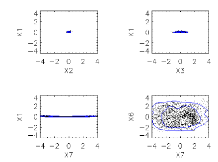
Figure 4: 1 and $2\sigma$ contours for pairs of principal components. Since they are linear combinations of standardized variables, they are all centered on zero. It is obvious these are plots of non-correlated parameters. The low scattering in the $X_{1}$ direction indicates that the cosmological parameters combination defined by $X_{1}$ is strongly constrained. On the other hand, the high scattering in the principal components associated with the highest eigenvalues, indicates these components contain most of the sample dispersion, and determine the cosmological parameters errors.

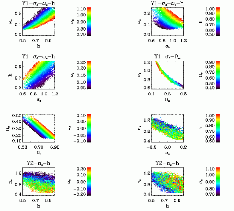
Figure 5: 2-dimensional scatter plots colored by a third parameter putting in evidence the multi-dimensionality of the degeneracies. Panels are numbered from top left to bottom right. Panels 1-3: Illustrate the best determined pc in the form $\omega_{c}-\sigma_{8}-h$. The well defined continuous gradients in all 3 cases show the existence of a degeneracy, even though that would not be obvious from the 2-dimensional projections alone. Panel 4: Using $\Omega_{m}$ instead of $\omega_{c}$, the best determined pc already defines a narrow degeneracy in the 2-dimensional plane $(\Omega_{m},\sigma_{8})$. $\Omega_{v}$ values are also shown. Panel 5: Coloring the $(\Omega_{v},\Omega_{m})$ plot with the curvature values, a linear pattern appears. Panel 6: Shows the degeneracy $\alpha_{s}-n_{s}$ which was not clear from the eigenvectors table alone. By coloring with $h$ it also shows that this degeneracy contributes to $Y_{2}$. Panels 7,8: The second best determined pc relates mainly $n_{s}$ and $h$. These plots show it also has some correlation with $\alpha_{s}$ (panel 7) and less from $\sigma_{8}$ (panel 8).

The most accurate PCS are the best determined quantities by the CFHTLS-wide cosmic shear experiment. In order to see to which combinations of cosmological parameters they correspond, one can look at the eigenvectors components, i.e., a high coefficient $a_{ij}$ means $p_{j}$ strongly contributes to $X_{i}$. However, since we are working with standardized parameters, the direct reading of the coefficients may be misleading. In fact, if we take any subset of 2 parameters and compute its eigenvectors, they both will have equal components, which obviously does not mean each principal component has equal contributions from each parameter. Hence, for the purpose of obtaining a set of meaningful coefficients , it is adequate to rescale the parameters differently. We rescale them by subtracting the mean and dividing by the mean. This is refered to as the fractional data in Chu et al. (2003). The covariance matrix of the rescaled sample relates to the original covariance matrix as, $C^{\prime}_{ij}=C_{ij}/(<p_{i}><p_{j}>).$

We compute a set of principal components, $Y$, from the fractional covariance matrix, expressed as,

$$Y_{i}=\sum_{j=1}^{7}\,b_{ij}{(p_{j}-<p_{j}>)\over<p_{j}>}.$$ (22)

Each $Y_{i}$ approximately corresponds to one $X_{i}$ but they are not equivalent since the principal components depend on the scaling of the variables. We show this set in Table 4 (III), computed for a slightly different set of cosmological parameters with $(\omega_{b},\omega_{c})$ replaced by $(\Omega_{b},\Omega_{m})$.

4.1.1 Well constrained PCS

The components of an eigenvector explicitly show the contribution of each parameter to a principal component:

• The first one, $Y_{1}$, is dominated by contributions from $\sigma_{8}$ and $\Omega_{m}$. This is the well known $\sigma_{8}-\Omega_{m}$ degeneracy. $\Omega_{v}$ is also non-negligible. Its presence here comes from its correlation with $\Omega_{m}$ through the prior on the curvature used to compute the chains (see Table 3).

• The second best constrained direction, $Y_{2}$, couples the primordial spectrum index, $n_{s}$, with $h$ and $\Omega_{m}$. This comes from the correlation between the tilt $n_{s}$ and the parameterisation of the slope of the mass power spectrum to which the shear is sensitive, $\Gamma=\Omega_{m}\,h$. Notice the coefficients of $n_{s}$ and $h$ have the same sign, as is also the case with $\sigma_{8}$ and $\Omega_{m}$ in $Y_{1}$, which shows the orientation of the degeneracy.

The relative contribution of the main parameter involved in each principal component is in the last column of Table 4 (III). For example, the projection of $Y_{1}$ on the direction of its main parameter ($\sigma_{8}$) is $78\%$. Although these fractions may be important, they are significantly below 100%, showing that none of these principal components that describe the cosmic shear spectrum depends on a single cosmological parameter.

The 2-dimensional projections of Fig. 5 use colors to produce 3-dimensional plots that better describe sensitivity of cosmic shear to cosmological parameters. The comparison of Table 4 (II) and Table 4 (III) shows for example that the $\sigma_{8}-\Omega_{m}$ degeneracy is equivalent to a $\omega_{c}-h-\sigma_{8}$ degeneracy. A scatter colored plot, like the top panels of Fig. 5, illustrates this in a simple way. On this figure, we plot the sample points for the 3 possible pairs of parameters, colored by the one left out. The continuous gradient along the third parameter is obvious. In particular, the degeneracy that is hidden in the $\sigma_{8}-\omega_{c}$ plane becomes evident once the points are colored according to $h$. Likewise, the cosmic shear $\sigma_{8}-\Omega_{m}$ degeneracy pattern $\sigma_{8}\propto\Omega_{m}^{-0.5}$ is shown on the fourth panel, with a continuous gradient along $\Omega_{v}$. The fifth panel shows how this correlation between $\Omega_{m}$ and $\Omega_{v}$ is related to the curvature.

The color plots also help in understanding degeneracies derived from the analysis of Table 4. The bottom panels of Fig. 5, illustrate the cases on the $Y2$ term either when a third parameter does not contribute to the degeneracy ($\sigma_{8}$) (producing a mixture of colors), or when it does ($\alpha_{s}$). The analysis of Table 4 alone is indeed confusing: while from 4 (III) it is not evident that $\alpha_{s}$ contributes more to the second principal component than $\sigma_{8}$ does, Table 4 (II) shows what really happens. The need for a careful interpretation of this table is of primarily importance when fractional covariance matrix is used for parameters with fiducial values close to zero. The simple extraction of eigenvectors components to find degeneracies only provides qualitative insight since there is no unique set of principal components. For these ambiguous cases, color plots are very useful. The bottom right panels of Fig. 5, reveal the sensitivity of $Y2$ to $\alpha_{s}$ in a much better way than the tables do.

From the MCMC and the principal components analysis, it is possible to describe some cosmic shear denegeracies with empirical laws, using the best determined components $Y_{1}$ and $Y_{2}$. Since the 2-dimensional contours of $Y_{1}$ and $Y_{2}$ are not ellipses, we made a new eigenvector calculation, using the logarithm of the parameters. The laws are established for two parameters only, marginalising over the others. This way we found the shapes in the $\sigma_{8}-\Omega_{m}$ and the $n_{s}-h$ planes to be:

$$\sigma_{8}\,\Omega_{m}^{0.52}=0.467\pm 0.008$$ (23)

and $h\,n_{s}^{0.57}=0.67\pm 0.10$. Defining $\Gamma=\Omega_{m}\,h$, we find a better constrained, $Y_{2}$ related, two parameter relation,

$$\Gamma\,n_{s}^{0.6}=0.187\pm 0.037.$$ (24)

4.1.2 Poorly constrained PCS

As for the other principal components:

• $Y_{3}$ is dominated by $\Omega_{v}$, $\Omega_{m}$ and $\sigma_{8}$. This constrains the curvature, mixed with an $Y_{1}$ orthogonal contribution of $\sigma_{8}-\Omega_{m}$, as the coefficients of these 2 parameters have now opposite signs.

• The projection of $Y_{4}$ on the $n_{s}-h$ plane constrains an orthogonal direction to the $Y_{2}$ projection.

• $Y_{5}$ mixes almost all the parameters, while being dominated by an $\Omega_{m}-\Omega_{v}$ plane orthogonal direction to the one defining the curvature. As we will see next, $Y_{5}$ alone is almost enough to determine the parameters precision.

• The two worst constrained principal directions,$Y_{6}$ and $Y_{7}$, are the most aligned ones with single parameters, being strongly dominated by $\Omega_{b}$ and $\alpha_{s}$, respectively.

Even though the best determined PCS give strong constraints on certain combinations of parameters, constraints on individual cosmological parameters are strongly dependent on the worst determined PCS, exception made for a cosmological parameter aligned with a well constrained principal component (from the last column of Table 4 (III) we see there is no such case). In fact, the worst constrained PCS determine the size of the hyper-volume defined by the sample in parameter space and account for most of the dispersion of the sample. This is the reason why $\Omega_{b}$ and $\alpha_{s}$, which dominate $Y_{6}$ and $Y_{7}$, are the worst determined parameters (Table 4 (I)). To investigate the contribution of each principal component to the one-dimensional errors on parameters, we compute the $1\sigma$ marginalised parameters dispersion using only a restricted number, $n$, of principal components, as:

$$\sigma^{2}(p_{j},n)=<p^{2}_{j}>\sum_{l=7}^{8-n}\,(Y_{l}\,b_{lj})^{2}.$$ (25)

Notice the case $n=1$ uses only $Y_{7}$. Notice also the need to multiply by the parameters means, since we are using fractional data. Table 4 (IV) shows the $1\sigma$ marginalised errors for each parameter as a percentage of the total $1\sigma$ marginalised errors (shown in Table 4(I)), computed in this way, where #pc=i refers to $n=i$ of Eq. (25). We see that $Y_{7}+Y_{6}+Y_{5}$ (#pc=3) accounts for over 95% of several parameters $1\sigma$ values and from $Y_{7}+Y_{6}+Y_{5}+Y_{4}+Y_{3}$ all the correct values are obtained. Hence, we may conclude that the statistical information of the sample can be reduced to 5 dimensions plus 2 narrow priors defined by $Y_{1}$ and $Y_{2}$. This way, a 5 dimensional MCMC would be enough to obtain an equivalent sample in a faster way.

Finally, the cosmic shear dependence on the cosmological parameters may be summarized in a single expression analogous to Eq. (12). It is derived by using the surface of least dispersion defined on the 7-dimensions surface. It must be orthogonal to $Y_{1}$, i.e., defined by $Y_{1}=c^{te}$. This constant is proportional to the cosmic shear variance signal from all scales (since they were all integrated to compute the likelihood, it does not explicitly depend on angular scale). We found that

$$\gamma\propto\sigma_{8}\,\Omega_{m}^{0.57}\,\Omega_{b}^{0.007}\,\Omega_{v}^{0.18}\,h^{-0.02}\,n_{s}^{-0.02}\,\alpha_{s}^{-0.002}.$$ (26)

The MCMC and principal component analysis of CFHTLS cosmic shear data alone can be generalised with joint data sets. As it has been shown in this section, the method provides useful information on degeneracies and principal components and allows a description of orthogonal directions. Used jointly with CMB data sets, we can therefore predict how CFHTLS cosmic shear and CMB data can be used in an optimal way to shrink the exclusion diagrams attached to each cosmological parameters.

5 Constraints from Cosmic Shear and CMB

We produced a different set of chains, computing the joint likelihood of the models with respect to the same cosmic shear fiducial data and CMB data.

We used the WMAP first year data: the combined TT power spectrum (Hinshaw et al. (2003)) and the TE power spectrum (Kogut et al. (2003)). Model’s likelihoods with respect to WMAP data were computed using the WMAP likelihood code (Verde et al. (2003)). In order to have information from smaller scales, we included CBI data: the mosaic odd binning (Pearson et al. (2003)).

Table 5: One-dimensional results from the joint sample. The errors are $1\sigma$. Above the horizontal line are the 7 explicitly changed MCMC parameters, while results for some other popular parameters are shown under the line. The column labeled $g_{1}$ shows the gain in the parameters precision in relation to the values obtained with the CMB chains. In the last column, the gain $g_{2}$ is computed in relation to available CMB results (taken from Table 8 of Spergel et al. (2003), for the case WMAPext).

	joint	$g_{1}$	$g_{2}$
$\omega_{b}$	$0.0224\pm 0.0008$	1.4	1.2
$\omega_{c}$	$0.112\pm 0.003$	3.6
$h$	$0.71\pm 0.02$	1.9	2.9
$n_{s}$	$0.94\pm 0.03$	1.7	2.0
$\alpha_{s}$	$-0.050\pm 0.018$	1.7	2.1
$10^{9}\,A_{s}$	$2.8\pm 0.2$	1.1
$\tau$	$0.24\pm 0.04$	1.0	1.7
$\Omega_{m}$	$0.26\pm 0.02$	2.8
$\sigma_{8}$	$0.91\pm 0.03$	2.5
$\Omega_{m}\,h$	$0.188\pm 0.008$	3.2
$\sigma_{8}\,\Omega_{m}^{0.5}$	$0.47\pm 0.01$	6.7  (1.1)
$\sigma_{8}\,e^{-2\,\tau}$	$0.56\pm 0.03$	1.8

Figure 6: Marginalised distributions for the cosmological parameters from the joint likelihood chains (solid line) and the CMB chains (dashed line).

The number of independent parameters explored by the Markov chains was kept at 7: $(\omega_{b}\,,\omega_{c}\,,h\,,n_{s}\,,\alpha_{s}\,,\tau\,,A_{s})$. The normalization is now parameterized by $A_{s}$, with a fiducial value of $A_{s}=2.6\times 10^{-9}$, corresponding in our fiducial model to $\sigma_{8}=0.9$. We restrict to flat models, hence $\Omega_{v}$ is no longer an independent parameter and let $\tau$, the optical depth to reionization, change in the restricted region of $\tau<0.3$., keeping its fiducial value at $\tau=0.17$.

We present results from a combination of 8 converged chains about $70\times 10^{3}$ elements long from which we rejected the first $30\times 10^{3}$ elements. The thinning factor is 8, leaving us with a final merged sample of about 40 000 elements.

Table 5 shows one-dimensional marginalised results from the joint sample. In order to explicitly see what can be gained when joining cosmic shear data to CMB data, we also produced CMB only chains. One-dimensional distributions from both CMB and joint samples are shown in Fig. 6. The ratio between the parameters standard deviations obtained with the CMB sample and the joint sample, $g=\sigma(CMB)/\sigma(CFHTLS+CMB)$, tells us to which parameters the combined analysis is more efficient. These values are shown in column $g_{1}$ of Table 5. As a consistency check we show in column $g_{2}$ the factor gained by the joint sample when compared with the most appropriate case of the published WMAP results. The largest gain is on the cluster abundance scaling, $\sigma_{8}\,\Omega_{m}^{0.5}$. As we saw, this parameter is roughly the first principal component of the cosmic shear and its error is well determined by cosmic shear alone. So, what makes more sense here is to compute the gain with respect to the cosmic shear sample and not to the CMB sample. In this case we find the joint sample brings no gain $(g_{1}=1.1)$.

Keeping in mind that the combined result of 2 independent experiments with errors of the same order has already a gain of $\sqrt{2}$, we consider the combined analysis to be efficient for a certain parameter if $g>\sqrt{2}$. Hence, the efficiency is higher for the dark matter density, the hubble parameter, $\sigma_{8}$ and the spectral indexes. To illustrate this result, we plot in Fig. 7 the pairs of parameters where the orthogonality between CMB and CFHTLS contours is most striking, among all possible pairs. These are contours of equal likelihood, containing $68\%$ and $95\%$ of the sample. All the 4 cases involve only the efficient parameters. Furthermore, they correspond to cosmic shear $Y_{1}$ and $Y_{2}$ related well constrained cases we found in the previous section. Thus, we found that projections of the best constrained cosmic shear principal components are orthogonal to the corresponding CMB contours, which shows a complementarity between cosmic shear and CMB.

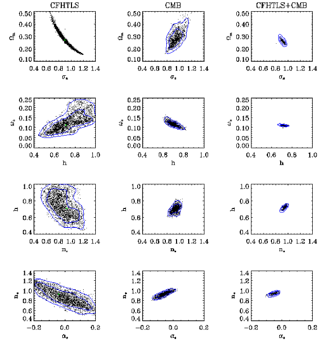
Figure 7: Marginalised 2-dimensional $68\%$ and $95\%$ contours from the three samples. These are the most relevant plots to illustrate the largest gains on the parameters precisions.

Figure 8: Primordial power spectrum parameterized by $n_{s}$ and $\alpha_{s}$. The values written in the panel titles define the dotted lines, while, in each panel, the solid lines are plotted with the fiducial values $(n_{s}=0.93\,\alpha_{s}=-0.04)$. The scale ranges probed by the CMB and the cosmic shear are shown in the upper left panel.

To understand the origin of some of this complementarity, let us consider the $n_{s}$/$\alpha_{s}$ case. The gain on both parameters is around 2, even though, as we saw, the cosmic shear by itself is not very sensitive to the running spectral index. In Fig. 8 we plot the primordial power spectrum from Eq. (3) as function of the linear wavenumber. The spectral indexes parameterize the shape of the spectrum and have no further role on its evolution. Thus the opposite behaviour of the CMB/cosmic shear responses to a change on the indexes may be understood from these plots. The solid line in all panels is the fiducial model $(n_{s}=0.93\,,\alpha_{s}=-0.04)$. It bends away from a power law ($\alpha_{s}=0$, the dashed line on the upper left panel) from the pivot point. The dotted lines are deviations from the fiducial model, they correspond to the indexes values written as the panels titles. In the top panels one parameter is changed at a time. On the left, a change on $n_{s}$ produces changes of opposite signs at both ends of the spectrum. On the right, changing $\alpha_{s}$ raises both ends of the spectrum. The bottom panels show how it is possible to mimic the fiducial spectrum for large (small) scales by changing both indexes in the same (opposite) direction.

On the first panel, the solid horizontal lines show the scale ranges probed by the CMB (the line on the left) and the cosmic shear (on the right) data used in this work. These intervals were found by using the calculations of Tegmark & Zaldarriaga (2002), in particular their fitting $k\approx\sqrt{(}3^{\prime}/\theta)\,[h/Mpc]$. Hence, the 2 bottom plots lead to expect an upper left - lower right direction of degeneracy for the cosmic shear and an orthogonal one for the CMB.

The shape of the $n_{s}/h$ lensing degeneracy has a similar origin. The slope of the power spectrum at the scales probed by the cosmic shear is $\Omega_{m}\,h$. A raise of $h$, increases the power at small scales that must be compensated by a decrease in $n_{s}$.

In order to have an explicitly view of the cosmic shear $n_{s}/\alpha_{s}$ degeneracy scale dependence, we produced a new set of 4 cosmic shear MCMC chains. This time, we only allowed the scalar spectral indexes to change and kept the other 5 of the 7 original parameters (see Table 3) at the fiducial values. The chains were built following the procedure detailed in section 3. Due to the small number of parameters probed, convergence was very rapid and a burn-in of 300 elements was enough to reach the equilibrium. The models shear dispersion and likelihood were computed for 4 cases, distinct on the angular scales used. These are (in arc minutes):

• ”small” scales: $(0.6,1,1.3,2,3,4,5,6)$

• ”medium” scales: $(8,10,15,20,25,30)$

• ”large” scales: $(40,50,60,80,100,120)$

• ”all”: all the above 20 angular scale points, which are the ones used in the 7-dimensional MCMC cosmic shear chains.

Figure 9 plots the sample points and contours obtained. It shows that even inside the comparatively small region of Fig. 8 probed by the cosmic shear, the scale dependency of the $n_{s}/\alpha_{s}$ degeneracy constraint is detected, with the best constraint coming from the smallest scales. The signal from the largest of the cosmic shear scales is more dispersed as it is shown at the bottom left panel of Fig. 9. Notice, in this case, the orientation of the contours is cut by the MCMC exploration limits imposed.

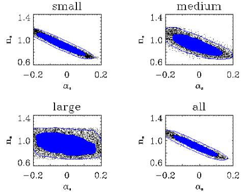
Figure 9: $n_{s}\,\alpha_{s}$ MCMC sample points and $68\%$ and $95\%$ confidence levels. The models likelihoods were evaluated using 4 different sets of angular scales - small, medium, large and all, defined in the text. The ”small” case is the one that better constrains the $n_{s}\,-\alpha_{s}$ degeneracy found in the 7-dimensional analysis.

There are parameters for which no gain was found, for instance, the measurement of $\omega_{b}$ is dominated by the CMB. For $\tau$, even though the cosmic shear is not sensitive to it, the introduction of cosmic shear data strengthens the $\sigma_{8}-\tau$ correlation allowing to lower the errors on $\sigma_{8}\,e^{-2\,\tau}$ (Table 5). Thus, even though we do not predict a gain on the measurement of $\tau$ from CFHTLS+CMB data, future cosmic shear surveys, through a more precise measure of $\sigma_{8}$, will be helpful in its determination. In Fig. 10 its is shown the correlation between $\sigma_{8}$ and $e^{-2\,\tau}$, the factor by which the CMB at small scales is damped after reionization. The information provided by the cosmic shear is clear.

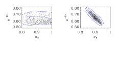
Figure 10: Marginalised 2-dimensional $68\%$ and $95\%$ contours.The first plot is from the CMB sample and the second one from the joint sample.

6 Discussion

We studied the determination of cosmological parameters by a CFHTLS-Wide type of experiment. For this we have made some assumptions that may not exactly match the real situation. First of all, the real survey features will not be identical to the used ones. In particular, we made the optimistic assumption that all the $170\,\rm{deg}^{2}$ of the survey area will be usable, whereas a size of $130\,\rm{deg}^{2}$ would be more realistic. Furthermore, since we assumed the redshift of the sources perfectly known, there will be an extra source of error coming from the marginalisation over the real sources redshift distribution. The same happens with the marginalisation over other cosmological parameters not taken into account in this study, such as the equation of state of dark energy or the neutrinos density. The calculations into deep non-linear regime using the halofit formula may also bring an extra source of errors.

We need also to keep in mind that we made a systematics-free study, with data errors being dominated by Poisson noise and cosmic variance. B-mode contamination due to systematic residuals could significantly increase uncertainty in the noise correction process and on the way it should be handled in the covariance matrix. However, it has recently been shown that the residual B-mode on the Virmos-Descart data could be further corrected and eventually set to zero. This result follows from a better understanding of the PSF variation across the CCD chips (see Hoekstra (2004) and Van Waerbeke et al. (2004)) and it is expected that the CFHTLS will be at least as good as Virmos-Descart in terms of image quality, hence we set B-modes to zero in this work.

On the other hand, our exploration of cosmological parameters is more realistic and accurate than previous studies. We use a non-diagonal data covariance matrix, allowing for correlation between scales. Furthermore the MCMC method probes the real shape of the posterior PDF, without assuming a gaussian distribution. It is also important to stress that the 2-points correlation functions do not contain all the cosmic shear information. In particular, we did not use higher order statistics, like the already detected convergence skewness (Pen et al. (2003)) or the three point shear correlation functions (Bernardeau et al. (2002)), that may help also to break degeneracies (Bernardeau et al. (1997)).

We explored the cosmological parameters space using cosmic shear, describing the results in the context of a principal components analysis, and found a set of parameters degeneracies orthogonal to CMB ones. This led to predict a gain of the order of 2 or 3 for several parameters, when combining CFHTLS-Wide data with WMAP and CBI data. This means, for example, precisions of $\sigma(\sigma_{8})=0.03$ and $\sigma(\Omega_{m})=0.02$. This result is consistent with the parameters determinations of Contaldi et al. (2003) that combines CMB data with the Red-Sequence Cluster Survey (RCS) data, where they found $\sigma(\sigma_{8})=0.05$ and $\sigma(\Omega_{m})=0.03$. From a quick Fisher matrix calculation, the ratio between parameters errors determined by 2 cosmic shear experiments is approximately given by a ratio of the experiments survey areas (A), galaxy densities (n) and intrinsic ellipticity dispersions ($\sigma$) (see for example Hu & Tegmark (1999)):

$$g_{cs}=\left({{A_{1}\,n_{1}^{2}\,\sigma_{2}^{4}}\over{A_{2}\,n_{2}^{2}\,\sigma_{1}^{4}}}\right)^{1\over 2}.$$ (27)

The ratio between CFHTLS-Wide and RCS (with a size $A=53\,\rm{deg}^{2}$) is 1.8.

As compared to the fiducial reference survey used by Ishak et al. (2003), this simple estimation predicts the precisions obtained with their reference survey should be 4 times better than the ones from our configuration. But we find the same, or only slightly bigger, $\sigma$ values. First of all, Eq. (27) gives only an upper limit for the combined gain. In fact, for a parameter whose determination is dominated by CMB, the cosmic shear contribution to the joint result must be smaller than this value. The main reason for this discrepancy is, however, the fact that our degraded configuration, as compared to the survey in Ishak et al. (2003), is partly compensated by the inclusion of smaller angular scales. In fact, we saw that it is in the non-linear regime that lies, not only the cosmic shear greatest sensitivity to the cosmological parameters, but also the cause of its orthogonality to CMB.

7 Conclusions

The CMB/cosmic shear complementarity opens good prospectives for the determinations of cosmological parameters by combining CMB and cosmic shear data sets. In fact, even for CFHTLS, whose contours are, in general, noticeably larger than the WMAP+CBI ones (Fig. 7), we predict non neglectable gains. Figure 11 shows what can be expected with future space telescope data.

Table 6: Cosmic shear : Wide field space telescope illustration specifications.

Size of the survey:	A=$1000\,{\rm deg}^{2}$
Density of galaxies:	$n_{g}=50\,{\rm arcmin}^{-2}$
Intrinsic ellipticity dispersion:	$\sigma_{\epsilon}=0.3$
Scales probed:	$0.6\,^{\prime}<\theta<5\deg$
	$40<l<18000$

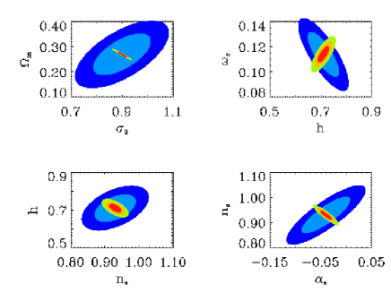
Figure 11: 68% and 95% C.L. for the 4 most orthogonal cases found in section 5. Blue is WMAP+CBI data and red shows predictions for the wide field space telescope - cosmic shear parameters of Table (6) (99 % C.L. is also shown in this case).

These results were produced with a cosmic shear Fisher matrix analysis, using Eq. (17) and the fiducial model of Table 1 (except for the redshift of the sources which was moved to $z_{s}=1.1$). For this illustration, the data covariance matrix of Eq. (2) was computed for the configuration shown in Table 6, which is close to the SuperNova Accelerator Probe / Joint Dark Energy Mission (SNAP/JDEM) ”Wide+” case of Réfrégier et al. (2003). The CMB ellipses are plotted from the parameters covariance matrix found with our WMAP+CBI chains.

In summary, we found the best constrained parameters by 2-point cosmic shear correlation functions to be $\sigma_{8}\,\Omega_{m}^{0.5}$ and $\Gamma\,n_{s}^{0.6}$ (with $\Gamma=\Omega_{m}\,h$). We have shown that 2-dimensional degeneracies defined by these parameters plus another one defined by $n_{s}$ and $\alpha_{s}$ are orthogonal to CMB degeneracies. Due to this CMB/cosmic shear complementarity, current weak lensing surveys, such as the CFHTLS, already have the potential to improve the precision on several cosmological parameters. In particular, a better knowledge of $\alpha_{s}$ will have an impact on inflationary scenarios. The crucial information provided by the cosmic shear comes from the small scales it probes. Thus, it provides an additional possibility, along with galaxy redshift surveys and Lyman-$\alpha$ forest, to combine with CMB data.