Is the slope of the intrinsic Baldwin effect constant?

Abstract

We investigate the relationship between emission-line strength and continuum luminosity in the best-studied nearby Seyfert 1 galaxy NGC 5548. Our analysis of 13 years of ground-based optical monitoring data reveals significant year-to-year variations in the observed H$\beta$ emission-line response in this source. More specifically, we confirm the result of Gilbert and Peterson (2003) of a non-linear relationship between the continuum and H$\beta$ emission-line fluxes. Furthermore, we show that the slope of this relation is not constant, but rather decreases as the continuum flux increases. Both effects are consistent with photoionisation model predictions of a luminosity-dependent response in this line.

1 Introduction

Observations of correlated continuum and broad emission-line variations in Active Galactic Nuclei (AGN) provide powerful diagnostics of the structure and physical conditions within the spatially unresolved broad emission-line region (BLR) and of the origin and shape of the unobservable ionising continuum.

A well-established correlation is the observed decrease in broad emission-line equivalent width with increasing continuum level for AGN spanning a broad range in continuum luminosity; this is the so-called global “Baldwin effect” (Baldwin 1977; Osmer, Porter and Green 1994). Originally observed in the strongest UV resonance lines (e.g. CIV$\lambda 1549$ and Ly$\alpha$), a global Baldwin effect has now been found for most of the strong UV emission-lines. Interestingly, evidence for a similar effect in the broad optical hydrogen recombination lines remains weak.

In a recent study of composite quasar spectra spanning a broad range in continuum luminosity and redshift, Dietrich et al. (2003) found no evidence for evolution of the Baldwin effect with cosmic time. Instead they suggested that the effect is a consequence of luminosity-dependent spectral variations, in the sense that the ionising continuum becomes softer for higher continuum luminosities. This agrees well with the theoretical work by Korista et al. (1998), who showed that if the gas metallicity and continuum spectral energy distribution are related statistically to the quasar luminosity, then so will be the emission-line equivalent widths, in a manner described by the Baldwin effect.

Formally, the relationship between the continuum luminosity ($L_{cont}$) and broad emission-line luminosity ($L_{line}$) may be represented by a single powerlaw, such that

$$L_{line}\propto L_{cont}^{\alpha}\,.$$ (1)

In terms of the line equivalent width, the Baldwin relation is then given by

$$EW_{line}\propto L_{cont}^{\beta}\,,$$ (2)

where $\beta=\alpha-1$. The measured values of $\alpha$ are typically $<1$, for example, $\alpha\approx 0.83$ for CIV and $\alpha\approx 0.88$ for Ly$\alpha$ (see e.g. Kinney, Rivolo & Koratkar 1990, Pogge & Peterson 1992), with corresponding slopes for the Baldwin relation of $\beta=-0.17$, and $\beta=-0.12$ respectively.

Figure 1: (Upper panel)$F(\lambda 5100\AA)$ continuum light curve (observed frame) for the full 13 yr AGNWatch monitoring campaign of NGC 5548. (Lower panel) The corresponding H$\beta$ emission-line light curve.

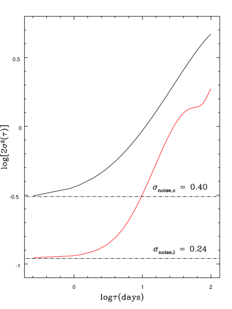
Figure 2: Computed structure functions for the continuum (upper curve) and H$\beta$ light curves. Dashed lines indicate the noise level in each of the light curves.

Superposed on the global Baldwin relation, is a second relation whose slope reflects the emission-line response to variations in the ionising continuum within an individual source. Now commonly referred to as the “intrinsic Baldwin effect”, this phenomenon accounts for at least some of the scatter seen in the global Baldwin relation. However, the intrinsic Baldwin relation also shows considerable scatter, whose origin is largely attributable to continuum–emission-line time-delay effects (reverberation) within the physically extended broad emission-line region (see e.g. Krolik et al. 1991, Pogge and Peterson 1992, Peterson et al. 2002).

Formally, the relationship between the continuum flux $F_{\rm cont}$ and emission-line flux $F_{line}$ within a single source can also be represented by a single powerlaw, such that

$$F_{line}\propto F_{cont}^{\alpha}\,,$$ (3)

where in this case $\alpha$ is a measure of the instantaneous emission-line response to changes in the ionising continuum flux, the responsivity of the gas. In terms of the line equivalent width, the intrinsic Baldwin relation is then given by

$$EW_{line}\propto F_{cont}^{\beta}\,.$$ (4)

where again $\beta=\alpha-1$.

While a global Baldwin relation has yet to be seen in the optical recombination lines, there is no physical reason why an individual source should not display an intrinsic Baldwin effect in these lines. That is to say, the broad range in physical conditions extant within the BLR are such that case B recombination, for which $\alpha\equiv 1$, does not apply. Indeed, Gilbert & Peterson (2003) recently reported just such an effect for the broad H$\beta$ emission-line in a comprehensive study of 10 years of ground-based optical monitoring data on the nearby Seyfert 1 galaxy NGC 5548, taken as part of the AGNWatch collaboration. Interestingly, Gilbert & Peterson noted (their Figure 4) that during a low continuum flux state (year 4 of the monitoring campaign), the relationship between the continuum and H$\beta$ emission-line flux, appeared to change. However, since there was only one low flux state, they were unable to determine whether this change was a result of flux-dependent effects (e.g. photoionisation) or time-dependent effects (e.g. a renormalization of the intrinsic relation due to a change in composition, and/or distribution of the line-emitting gas).

While variations in the emission-line response with continuum state have long been predicted by photoionisation calculations (e.g. O’Brien et al. 1995; Goad 1995; Korista & Goad 2004), they have so far never been reported in the observations. Here, we take a detailed look at all 13 years of optical continuum and emission-line data available for NGC 5548, including two new low-flux states. Using this unique dataset we have found the first observational evidence for luminosity-dependent variations in the emission-line response. These luminosity-dependent variations are not only apparent in the whole dataset (reinforced by the addition of new low continuum flux data from years 12 and 13), but are even visible within individual observing seasons, being particularly prominent during those seasons displaying both high and low continuum flux states (e.g. year 4, see §3). Since the observed variations can occur on timescales of less than one year, they most likely represent a response to luminosity variations rather than to structural changes in the emission-line region.

2 13 yrs of optical data

The bright ($\lambda\/L(\lambda 5100\rm{\AA\/})\sim 10^{43.5}$erg s^-1), nearby (z=0.017), Seyfert 1 galaxy NGC 5548 is perhaps the best-studied of all AGN at optical wavelengths. This galaxy has been the subject of a concerted monitoring campaign by the AGNWatch collaboration since 1990, having been observed over 1500 times with a mean sampling interval of $\sim 3$ days (see e.g. Peterson et al. [2002] for a comprehensive review).

Here we analyse the optical continuum and H$\beta$ emission-line data for NGC 5548 in order to determine whether the H$\beta$ emission-line response for this source is sensitive to the continuum level throughout the 13 year duration of this campaign. For homogeneity, we use only data taken with the Ohio-State CCD spectrograph on the 1.8 m Perkins Telescope at the Lowell Observatory in Flagstaff Arizona. For a detailed review of the reduction procedure we refer the reader to Peterson et al. (2002) and references therein. In brief, the continuum flux was measured in a 10 Å wide bin centred at $\lambda$5100 Å in the rest frame of the galaxy. The H$\beta$ emission-line flux was then determined by integrating the flux over a linear fit to the background continuum between $\lambda$4710 Å and $\lambda$5100 Å again in the rest-frame of the galaxy. Figure 1 shows the full 13 years of continuum and line flux measurements (observed frame) taken as part of the AGNWatch campaign.

2.1 Background removal

Both continuum and emission-line fluxes are contaminated by nuisance background components which must be removed. The continuum flux measurements are contaminated by a constant background contribution by starlight from the host galaxy. In addition, the broad H$\beta$ emission-line flux is contaminated by a non-variable narrow-line component. For each component we adopt the canonical values used by Gilbert & Peterson (2003) in their fit to the first 10 years of the AGNWatch data ie. $F_{\rm galaxy}=3.37\pm 0.54\times 10^{-15}$ erg cm^-2 s^-1 Å^-1 for the continuum flux (Romanishin et al. 1995) and $F(H\beta_{\rm narrow})=6.7\pm 0.6\times$10^-14 erg cm^-2 s ^-1.

Figure 3: A section of the original continuum light curve (open squares) and the reconstructed continuum flux points (filled triangles) together with their associated uncertainties.

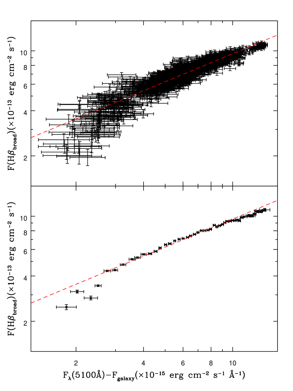
Figure 4: (Upper panel) Best-fit slope (dashed line) to the full 13 yrs of optical data. (Lower panel) As above, only this time we show the data binned in 0.25 intervals in continuum flux (see text for details).

2.2 Delay removal and error estimates from structure function analysis

The continuum and H$\beta$ light curves are highly correlated, but the emission line variations are delayed with respect to the continuum (Fig 1). Physically, these delays arise because the continuum is produced close to the central engine of an AGN whereas the line-forming region is located at larger distances, in the spatially extended BLR. Given that the line emission is ultimately powered by the continuum incident on the BLR, the lines thus respond to changes in the continuum with a time-delay, $\tau$, that is a measure of the luminosity-weighted radius, $R_{\rm BLR}$, of the BLR, ie. $\tau\simeq R_{\rm BLR}/c$.

When determining emission-line responsivities, these delays are contaminants and must be corrected for. This is because the line responsivity is defined as the instantaneous emission-line response to short-timescale small amplitude changes in the continuum flux incident on the BLR at the same time ie. $\alpha=d\log F_{line}/d\log F_{cont}$. In practice, we therefore shift the emission-line data for each year by their respective delays (as calculated from the centroids of the cross-correlation function for each of the 13 years of data, see e.g. Peterson et al. 2002). We then estimate the continuum flux at each (shifted) emission line epoch as the weighted average of the two bracketing continuum points.

The appropriate weight for each point is calculated from the first order structure function derived from the continuum light curve. Detailed descriptions of structure function analysis may be found in Kawaguchi et al. (1998) or Paltani (1999) and references therein. Briefly, the first order structure function for a series of flux measurements $f(t_{i})$, $i=1,N$ is defined as

$$S(\tau)=\frac{1}{N(\tau)}\sum_{i<j}[f(t_{i})-f(t_{j})]^{2}\,,$$ (5)

where the sum is over all pairs of points for which $t_{j}-t_{i}=\tau$, and $N(\tau)$ is the total number of pairs of points. It is straightforward to show that $S(\tau)$ is a measure of (twice) the variance of the light curve on timescale $\tau$, i.e. $S(\tau)\simeq 2\sigma^{2}(\tau)$. Correspondingly, structure functions are usually characterised by two flat sections with amplitudes of twice the total variance of the data, $2\sigma^{2}$, on the longest timescales and twice the noise variance due to observational errors, $2\sigma_{noise}^{2}$, on the shortest timescales. These flat sections are typically joined by by a rising power law on intermediate timescales.

Figure 2 shows the structure functions for both the continuum (upper curve) and emission-line (lower curve) light curves for timescales of $<$500 days. Given a pair of continuum points, the continuum structure function tells us immediately the correct weight to assign each point in estimating the continuum flux at any time, $t$, between them. More specifically, each of the two points bracketing $t$ is assigned the usual inverse variance weight $2/S(\tau)\simeq 1/\sigma^{2}(\tau)$, where $\tau=t_{i}-t$ and $t_{i}$ is the time associated with each point.

We also use the structure functions to estimate the errors on both emission-line and continuum flux estimates. Figure 2 shows that the structure functions are flat on the shortest timescales ($\tau\raisebox{-2.58334pt}{$\,\stackrel{{\scriptstyle\raisebox{-0.60275pt}{$\textstyle<$}}}{{\sim}}\,$}$ 1 day). The corresponding estimates of the instrumental uncertainties are $\sigma_{noise,c}=0.4\times 10^{-15}$ erg cm^-2 s^-1 Å^-1 for the continuum and $\sigma_{noise,l}=0.24\times 10^{-13}$ erg cm^-2 s^-1 for the line. These respectively correspond to fractional errors of $\sim 3$% and $\sim 2$% at high continuum and line flux levels, rising to $\sim 25$% and $\sim 15$% at low continuum and line flux levels. Since shifting the line data points leaves their flux values unaltered, we simply take the error on the line fluxes to be $\sigma_{l}=\sigma_{noise,l}$. By contrast, the reconstructed continuum points are two-point weighted averages of the bracketing data values. We therefore assign errors corresponding to the standard deviation estimated from these data values,

$$\sigma_{c}^{2}=\frac{2}{\sum_{i=1}^{2}\frac{1}{\sigma_{(}\tau_{i})^{2}}}.$$ (6)

The factor two in the numerator is needed because we want the standard deviation of the two bracketing points, not the error on the mean. This ensures that the minimum error associated with a reconstructed point is $\sigma_{noise,c}$ (rather than $\sigma_{noise,c}/\sqrt{2}$).

Figure 3 shows the input continuum (open squares), reconstructed continuum (filled triangles) and their associated errors for a small section of the 13 year light curve. Note that in filling data gaps of less than a day, our reconstruction assigns uncertainties comparable to those on the original data points (i.e., $\sigma_{noise,c}$). Where gaps are longer (e.g., boundaries between observing seasons) the uncertainties on the reconstructed points in the gaps increase with increasing distance from the nearest bracketing point. Both types of limiting behaviour are sensible.

3 Results

Figure 4 (upper panel) shows the $\lambda$5100Å continuum flux versus H$\beta$ emission-line flux after correcting for contaminating background components and the yearly continuum–emission-line time-delays. Also shown (dashed line) is a linear least squares fit to the data accounting for errors in both coordinates, and assuming that the data follow the relation

$$\log F({\rm H}\beta_{\rm broad})=\log A+\alpha\log[F_{\lambda}(5100\AA)-F_{galaxy}]\,.$$ (7)

The best-fit slope $\alpha$, and 1$\sigma$ uncertainty (estimated using bootstrap re-sampling) together with the mean continuum flux (unweighted) and root mean square error are given in Table 1. Our estimated slope and 1$\sigma$ uncertainty for the 13 year campaign, $0.621\pm 0.019$ (Table 1), is marginally smaller (but still within the estimated uncertainties) than that found by Gilbert and Peterson (2003) for the first 10 years of data. We therefore confirm Gilbert and Peterson’s finding of an intrinsic Baldwin effect for this line with slope $\beta\approx-0.4$.

Figure 4 – lower panel – shows the same relation plotted against the binned continuum data. The continuum data were binned in 0.25 intervals in continuum flux with individual points in each bin weighted according to the uncertainties on the reconstructed continuum flux. The binned continuum data indicate evidence not only for a steepening of the observed relation at low continuum flux levels, as previously noted by Gilbert and Peterson (2003), but also for a flattening of the relation at the highest continuum fluxes.

In order to discriminate between temporal changes in the structure of the BLR and a luminosity-dependent emission-line response, we have also applied the same fitting routine to each year of data separately. Figure 5 shows the best fit slopes (solid lines) for each of the 13 years of data. To guide the eye, we also show the best fit slope (dashed line) determined for the full 13 year campaign. The measured slopes and their 1$\sigma$ uncertainties (again determined using bootstrap re-sampling) are given in Table 1.

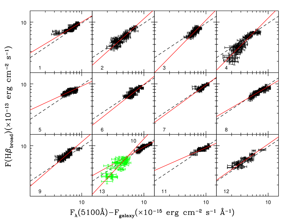
Figure 5: Best-fit line responsivities, $\alpha$, for each of the 13 years of optical data. To guide the eye, we also show the best-fit line responsivity (dashed line) for the complete data set. For ease of display, panel 10 contains fits to year 10 and year 13.

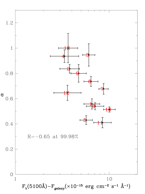
Figure 6: The measured correlation between the line responsivity $\alpha$, and continuum flux. The numbers indicate the corresponding observing season. A Pearson’s’ rank correlation shows that $\alpha$ is anti-correlated with continuum flux at better than $3\sigma$.

Table 1: The measured H$\beta$ emission-line responsivities, $\alpha$, and their 1$\sigma$ uncertainties for combined and yearly data sets. Also shown are the corresponding values for the intrinsic Baldwin relation $\beta$. Quoted flux values are the unweighted means and rms error in units of $10^{-15}$ erg cm^-2 s^-1 Å^-1.

Year	$\alpha$	$\beta=\alpha-1$	$\sigma_{\alpha}$	$<F_{cont}>$	$\sigma_{<F_{cont}>}$
			$\sigma_{\beta}$	($\times 10^{-15}$)
all years	0.621	$-$0.379	0.019	6.33	2.41
1	0.558	$-$0.442	0.041	6.54	1.27
2	0.836	$-$0.164	0.034	3.79	0.91
3	0.946	$-$0.054	0.089	6.06	0.92
4	0.936	$-$0.064	0.050	3.34	1.17
5	0.430	$-$0.570	0.035	5.69	0.87
6	0.736	$-$0.264	0.040	6.40	1.11
7	0.677	$-$0.323	0.042	8.71	1.01
8	0.540	$-$0.460	0.028	7.07	1.52
9	0.800	$-$0.200	0.070	4.73	0.89
10	0.514	$-$0.486	0.021	10.05	1.44
11	0.410	$-$0.590	0.041	8.48	1.82
12	0.646	$-$0.354	0.060	3.59	1.20
13	1.000	0.000	0.116	3.65	0.86

4 Discussion

Figure 5 and Table 1 demonstrate that the H$\beta$ emission-line responsivity, $\alpha$, shows significant variations from one observing season to the next. To quantify this further, we show in Figure 6 the mean continuum flux for each observing season versus $\alpha$ for each of the individual years. A Pearson’s rank correlation shows that $\alpha$ is anti-correlated with the optical continuum luminosity with slope $-0.65$ at better than $3\sigma$, strongly suggesting that the continuum luminosity and H$\beta$ line responsivity are intimately connected. Further corroborating evidence for such a relation can be seen in panel 4 of Figure 5. Season 4 displays the largest range in continuum variation of any of the 13 seasons. It also shows a marked increase in slope with decreasing continuum level. A similar trend though not as notable, is also seen in year 2. Such short timescale variations in the line-responsivity are unlikely to be due to dynamical effects within the BLR. The dynamical timescale $\tau_{dyn}$ for the BLR is given by $\tau_{dyn}\approx R/v_{\rm fwhm}$, where $R$ is the luminosity-weighted “size” of the BLR, and $v_{\rm fwhm}$ is the full-width at half-maximum of the root mean square emission-line profile. Adopting the mean BLR size of $\sim 20$ lt-days and mean FWHM of the H$\beta$ profile of $\sim$5000 km s^-1), $\tau_{\rm dyn}\approx 3$ yrs for this source, far longer than any single observing season.

Given the relatively short timescales over which changes in the emission-line responsivity occur, our preferred interpretation is that variations in $\alpha$ are likely related to changes in continuum flux only. While there are clearly points which do not obey this general trend, e.g. year 7, we suspect that this merely reflects our inability to adequately account for reverberation effects within the spatially extended BLR. For example, we expect the largest discrepancies from the overall trend in Figure 6 whenever a low continuum state directly follows a high one. This is due to a residual contribution to the overall response in the low state from emission-line gas in the outer BLR. The time delay associated with this region is longer than the luminosity-weighted average, so it may still be responding to the prior high-state continuum flux. Residual reverberation effects such as these most likely account for the comparatively weak response of the line during year 12, a low continuum state which follows two previous high continuum states (years 10 and 11).

We note that the measured line-responsivities presented here indicate the relationship between the integrated H$\beta$ emission-line flux and $\lambda 5100$Å continuum flux. However, to ascertain the mechanism behind this relation it is necessary to relate the emission-line flux to the ionizing continuum flux. Since we cannot observe the ionising continuum directly, we adopt the $\lambda 1350$Å continuum flux as a reasonable surrogate. Contemporaneous UV/optical continuum data (Gilbert & Peterson 2003) reveal a relationship of the form

$$F(\lambda 5100\AA)\propto F(\lambda 1350)^{2/3}\,.$$ (8)

Thus the slopes relative to the driving ionizing continuum may be up to a factor of 2/3 smaller than those presented here, ranging from $\sim 0.27$ at high continuum flux levels, to $\sim 0.67$ at low continuum flux levels.

An enhanced line-response at low incident continuum levels and a reduced line-response at high continuum levels matches well the predicted temporal behaviour of the optical recombination lines in recent detailed photoionisation calculations of the BLR in NGC 5548 (Korista and Goad 2004). The origin of this behaviour is thought to arise from the strong dependence of these lines’ emissivities on the incident ionising photon flux which results in a marked reduction in their responsivity with decreasing distance from the central ionising continuum source. Their responsivities should therefore display temporal variations due to large changes in the continuum luminosity, with their responsivities expected to be anti-correlated with the continuum level. This is in stark contrast to the behaviour of the high ionization lines (HILs) whose lines responsivities are more strongly correlated with the overall ionization state of the gas than on the incident ionising continuum flux. Since the line responsivity $\alpha$ is on average smaller for the optical recombination lines than for the HILs, we expect a stronger intrinsic Baldwin effect for these lines than for the HILs, as is generally observed (see e.g. Krolik et al. 1991; Pogge & Peterson 1992; Dietrich et al. 2003).

5 Conclusions

Our analysis of $\sim$13 years of optical continuum and H$\beta$ emission-line data for NGC 5548 shows that the H$\beta$ emission-line responsivity and hence slope of the intrinsic Baldwin effect $\beta$ displays significant variation on timescales $\sim 1$ yr. The line responsivity is generally anti-correlated with continuum level such that in high continuum states the emission-line response is weaker on average. Conversely in low continuum states the responsivity is stronger than on average. This behaviour is consistent with predictions of photoionisation models.

6 Acknowledgements

We would like to thank the referee, Ari Laor, for helpful comments leading to clarification of the key points presented in this work. MRG would also like to thank the generous hospitality of the family Korista during the initial stages of this work.

References

- [1] Baldwin, J. 1977, ApJ 214, 679.
- [2] Dietrich, M. et al. 2003, ApJ, 589, 722.
- [3] Gilbert, K.M. & Peterson, B.M. 200, ApJ 587, 123.
- [4] Goad, M.R. 1995, PhD Thesis University College London.
- [5] Kawaguchi, T. et al.1998, ApJ 504, 671.
- [6] Kinney, A.L., Rivolo, A.R., and Koratkar, A.P. 1990, ApJ 357, 338.
- [7] Korista, K.T., Baldwin, J.A. & Ferland, G.J. 1998, ApJ 507, 24.
- [8] Korista, K.T. & Goad, M.R. 2004, ApJ in press.
- [9] Krolik, J. et al. 1991 ApJ 371, 541.
- [10] O’Brien, P.T., Goad, M.R. and Gondhalekar 1995, MNRAS 275,1125.
- [11] Paltani, S. 1999, in ASP Conf. 5, BL Lac Phenomenon, ed. L. Takalo & A. Sillanpaa (San Francisco:ASP) 159, 293.
- [12] Peterson, B.M. et al. 2002, ApJ 581, 197.
- [13] Pogge, R.W. & Peterson, B.M. 1992 AJ 103, 1084.
- [14] Romanishin, W. et al. 1995, ApJ 455, 516.
- [15] Wanders, I. & Peterson, B.M. 1996, ApJ 466, 174.