Dust in Brown Dwarfs

Dust formation in brown dwarf atmospheres is studied by utilising a model for driven turbulence in the mesoscopic scale regime. We apply a pseudo-spectral method where waves are created and superimposed within a limited wavenumber interval. The turbulent kinetic energy distribution follows the Kolmogoroff spectrum which is assumed to be the most likely value. Such superimposed, stochastic waves may occur in a convectively active environment. They cause nucleation fronts and nucleation events and thereby initiate the dust formation process which continues until all condensible material is consumed. Small disturbances are found to have a large impact on the dust forming system. An initially dust-hostile region, which may originally be optically thin, becomes optically thick in a patchy way showing considerable variations in the dust properties during the formation process. The dust appears in lanes and curls as a result of the interaction with waves, i. e. turbulence, which form larger and larger structures with time. Aiming on a physical understanding of the variability of brown dwarfs, related to structure formation in substellar atmospheres, we work out first necessary criteria for small-scale closure models to be applied in macroscopic simulations of dust forming astrophysical systems.

1 Introduction

Substellar objects like brown dwarfs and (extrasolar) planets are largely - but not entirely - convective with considerable overshoot in the upper atmosphere. They also provide excellent conditions for the gas phase transition to solids or liquids (henceforth called dust). The understanding of such object’s atmospheres requires therefore the modelling of convection and, because the inertia of the fluid is larger than its friction (Re$\gg 10^{4}$), turbulent dust formation must be considered. Hence, substellar atmospheres involve various scale regimes with each being dominated by possibly different physical (e. g. streams, waves, precipitation) and chemical processes (e. g. combustion, dust formation, coagulation).

The large-scale structure of compact, substellar atmospheres is characterised by local and global convective motions (e. g. thunderstorms and monsoon like winds) and – simultaneously – by the gravitational settling of the dust. This scale regime has widely been investigated by 1D static, frequency dependent atmosphere calculations applying mixing length theory. The presence of dust in form of several homogeneous constituents has been modelled by applying local stability and time scale arguments (Rossow 1978, Borrows${\rm\hskip 3.44444ptet\hskip 3.01385ptal.\hskip 2.15277pt}$1997, Saeger${\rm\hskip 3.01385pt\&\hskip 3.01385pt}$Sasselow 2000, Ackermann${\rm\hskip 3.01385pt\&\hskip 3.01385pt}$Marley 2001, Allard${\rm\hskip 3.44444ptet\hskip 3.01385ptal.\hskip 2.15277pt}$2001, Tsuji 2002, Cooper${\rm\hskip 3.44444ptet\hskip 3.01385ptal.\hskip 2.15277pt}$2003). Recently, Woitke${\rm\hskip 3.01385pt\&\hskip 3.01385pt}$Helling (2003a; Paper II) have proposed a consistent treatment of nucleation, growth, evaporation and gravitational settling of heterogeneous dust particles, which has been applied for the first time to stellar atmosphere models in (Woitke${\rm\hskip 3.01385pt\&\hskip 3.01385pt}$Helling 2004; Paper III).

Modelling macroscopic scales, Ludwig${\rm\hskip 3.44444ptet\hskip 3.01385ptal.\hskip 2.15277pt}$(2002) have presented the first 3D simulations of M-dwarf convective atmospheres, applying the Large Eddy Simulation (LES) technique based on the experience of Nordlund & Stein with the solar convection. While the largest scales, which contain most of the energy and energise a small-scale turbulent fluid field, are computationally resolved, smaller scales are modelled by a hyperdiffusion which prevents the energy to accumulate in the smallest scales, thereby smoothing out all small-scale structures. Numerically, it stabilises the flow by filtering out sound and fast mode waves (see e. g. Caunt${\rm\hskip 3.01385pt\&\hskip 3.01385pt}$Korpi 2001).

Coming from the opposite site of the turbulent energy cascade, Helling${\rm\hskip 3.44444ptet\hskip 3.01385ptal.\hskip 2.15277pt}$(2001; Paper I) have investigated the dust formation process in the small, microscopic scale regime ($l_{\rm ref}\ll H_{\rho}$) by direct simulations of acoustic wave interactions. These investigations of the dense, initially dust-hostile layers in brown dwarf atmospheres have revealed a feedback loop which characterises the dust formation process:

The interaction of small-scale perturbations of the fluid field can cause a short-term temperature decrease low enough to initiate dust nucleation. The seed particles grow until they reach a size where the dust opacity is large enough to re-enforce radiative cooling which causes the temperature to decrease again below the nucleation threshold. Dust nucleation is henceforth re-initiated which results in a further intensified radiative cooling. The nucleation rate and consequently also the amount of dust particles increase further. This run-away process is stopped if either the radiative equilibrium temperature of the gas is reached or all condensible material is consumed. Meanwhile, the seed particles have grown to macroscopic sizes ($\mu$m).

Based on this knowledge, we extent our studies to larger and larger spatial scales aiming finally at the simulation of dust formation in the macroscopic scale regime, i. e., the complete atmosphere. The next step is therefore to study the mesoscopic scale regime ($l_{\rm ref}<H_{\rho}$) where we model driven turbulence by stochastically superimposed waves in the inertial Kolmogoroff range and study the response of the dust complex. Necessary criteria are derived for a small-scale closure model to be applied in large scale simulations of dust forming systems.

The aim of such a scale-wise investigation is to understand the major physical mechanisms which are responsible for the structure formation in the atmospheres of substellar objects and to provide the necessary informations for building an appropriate sub-grid model needed to solve the closure problem inherent to any macroscopic turbulence simulation (not only) of dust forming media (see also Canuto 1997a, 2000). The challenge is that only the largest scales of the turbulence cascade are comparable with real astrophysical observations but structure formation is usually seeded on the smallest scales especially if it is correlated with chemical processes. From the theoretical point of view, turbulence in thin atmospheric layers may be of quasi-2D-nature (Cho${\rm\hskip 3.01385pt\&\hskip 3.01385pt}$Polvani 1996, Menou${\rm\hskip 3.44444ptet\hskip 3.01385ptal.\hskip 2.15277pt}$2003). The 2D turbulence is characterised by an inverse energy cascade (transfer from small to large scales), contrary to 3D turbulence, which makes a scale-wise investigation even more urgent.

Various model approaches have been carried out to simulate and to study turbulence in different astrophysical scale regimes. For example, thermonuclear flames in type Ia supernovae have been studied on small scales by Röpke, Niemeyer & Hillebrandt (2003), investigating the Landau-Darrieus instability in 2D simulations which is responsible for the formation of a cellular structure of the burning front. Reinecke, Hillebrandt & Niemeyer (2002) have performed large-scale calculations in order to model supernovae explosions on scales of the stellar radius. Mac Low (1999; see also Mac Low${\rm\hskip 3.01385pt\&\hskip 3.01385pt}$Klessen 2004), for instance, have set up isothermal initial velocity perturbations with an initial power spectrum of developed turbulence in the Fourier space and initially constant density. They model decaying turbulence on the small scales of the inertial subrange. Smith, Mac Low & Heitsch (2000) use a similar approach but study the effect of driven turbulence in the same scale regime of star-forming clouds. A stationary but stochastic velocity field was applied by Wallin, Watson & Wylf (1998) in order to perform radiative transfer calculations of Maser spectra of a sub-parsec disk of a massive black whole. A fundamental theoretical investigation of the methods of driven turbulence is provided in (Eswaran & Pope 1987, 1988). A different approach of turbulence and convective modelling is followed by Canuto (e. g. 1997b) who treats turbulent convection by a Reynold separation ansatz where decomposed quantities (background field + fluctuations) are introduced into the model equations.

In this paper, we present a model for driven turbulence which allows us to study the onset of dust formation under strongly fluctuating hydro- and thermodynamic conditions in the mesoscopic scale regime. We thereby intend to model a constantly occurring energy input from the convectively active zone. Section 2 states the model problem and the characteristic numbers of our astrophysical problem. The turbulence model is outlined in Sect. 2.2. In Sect. 3, the results are presented for 1D simulations and an illustrative 2D example. Section 4 contains the discussion, and Section 5 the conclusions.

2 The model

The model equations for a compact substellar atmosphere are summarised. The model is threefold: i) hydro- and thermodynamics (Complex A), ii) chemistry and dust formation (Complex B; both Sect. 2.1), and iii) turbulence (Sect. 2.2). Our model philosophy is to study the dust forming system in different scale regimes in order to identify major mechanisms which might be responsible for cloud formation and possible variability in substellar atmospheres. The approach is based on dimensionless equations such that their solution is characterised by a set of characteristic numbers.

2.1 The model for a compressible, dust-forming gas

The complete set of model equations was outlined in detail in Paper I. Only a short summary is therefore give here.

Complex A: The hydro- and thermodynamics are described following the classical approach for an inviscid, compressible fluid; (Eqs.(1)–(5)) in Paper I.

Complex B: The chemistry and dust formation. The dust formation is a two step process – nucleation and growth (Gail${\rm\hskip 3.44444ptet\hskip 3.01385ptal.\hskip 2.15277pt}$1984; Gail & Sedlmayr 1988) – and depends through the amount of condensible species on the local density and chemical composition of the gas which are determined by Complex A. The nucleation rate $J_{*}$, which is strongly temperature-dependent, is calculated from Eq. (17) in Paper I applying the modified classical nucleation theory (Gail${\rm\hskip 3.44444ptet\hskip 3.01385ptal.\hskip 2.15277pt}$1984). The dust growth is described by the momentum method developed by (Gail${\rm\hskip 3.01385pt\&\hskip 3.01385pt}$Sedlmayr 1986, 1988; Dominik et al. 1993) in combination with the differential equations describing the element conservation (Eqs.(6)–(8) in Paper I).

Our model of dust formation considers a prototype-like phase transition (gas $\to$ solid) which is triggered by the nucleation of homogeneous ${\rm(TiO_{2})}_{N}$-clusters (see Jeong${\rm\hskip 3.44444ptet\hskip 3.01385ptal.\hskip 2.15277pt}$1998, Gail${\rm\hskip 3.01385pt\&\hskip 3.01385pt}$Sedlmayr 1998, Jeong${\rm\hskip 3.44444ptet\hskip 3.01385ptal.\hskip 2.15277pt}$2003). The formation of the dust particles is completed by the growth of a heterogeneous mantle which is assumed to be arbitrarily stable. The most abundant elements after H, C, O, and N in a solar composition gas are Mg and Si followed by Fe, S, Al, $\ldots$, Ti, $\ldots$ Zr. Therefore, the main component of the dust mantle can be expected to be some kind of silicate with a Mg/Si/O mixture plus some impurities. Since the focus of our work concerns the initiation of the dust formation in hostile turbulent environments rather than a detailed description of the growth process, evaporation and drift are neglected. Therewith, the maximum effects regarding the amount of dust formed in brown dwarf atmospheres is studied.

The most abundant Si bearing species in the gas phase under conditions of chemical equilibrium is the SiO molecule. Therefore, the collision rate with SiO can be expected to limit the growth of various silicate materials (like SiO₂, Mg_2xFe_2(1-x)SiO₄ and Mg_xFe_1-xSiO₃) rather than the collision rate with the nominal molecules (monomers) which are usually much less stable and hence barely present in the gas phase (Gail${\rm\hskip 3.01385pt\&\hskip 3.01385pt}$Sedlmayr 1999). Consequently, SiO is identified as the key species for the description of the growth of the dust mantles in our model (compare Paper II). In order to prevent an overproduction of seed particles, we furthermore include TiO₂ also as additional growth species, which leads to a quick consumption of Ti from the gas phase as soon as relevant amounts of dust are present.

2.1.1 Characteristic numbers and scale analysis

The use of dimensionless equations (Eqs. (1)–(8) in Paper I) provides the possibility to characterise the systems behaviour by non-dimensional numbers. The related estimations of typical time and length scales are summarised in Table 2 (Appendix A) for which the reference values only need to be known by orders of magnitude. It would, however, be very difficult to adopt an unique representation of the reference values from recent brown dwarfs model atmosphere calculation because of the differences among the different groups (compare Fig. 10). The agreement is nevertheless good enough that we consider them as typical, classical hydrostatic brown dwarf model atmosphere which lead our choice of reference values in Table 2.

Complex A:

– Assuming the typical turbulence velocity to be of the order of one tenth of the velocity of sound leads to a Mach number $M\approx\cal{O}$$(0.1)$. This choice has been guided by the results of Ludwig${\rm\hskip 3.44444ptet\hskip 3.01385ptal.\hskip 2.15277pt}$(2002) who derived a maximum vertical velocity of $\cal{O}$$(10^{4}\mbox{cm\,s${}^{-1}$})\approx c_{s}/10$ cm $s^{-1}$ which is about the same order of magnitude like the convective velocities derived from the mixing length theory (MLT). This value of a large-scale velocity does presently determine the energy dissipation rate (Eq. 3) of the turbulence model applied (Sect. 2.2) in this paper.

– The Froude number is $Fr=\cal{O}$$(10^{-2}\ldots 10^{-1})$ for a mesoscopic reference lengths $l_{\rm ref}<H_{\rho}$. Therefore, the pressure gradient and the gravity are now of almost comparable importance. However, gravity will gain considerable influence on the hydrodynamics only for scales regimes $l_{\rm ref}\geqslant H_{\rho}$ ($l_{\rm ref}=H_{\rho}\Rightarrow Fr=M$). The analysis of the characteristic combined drift number performed in Paper III (see Tables 2, 4 therein) has shown that the drift term in the dust moment equations is merely influenced by the gravity and the bulk density of the grains. We therefore assume also in the mesoscopic scale regime position coupling between dust and gas which seems reasonable due to the almost equal importance of the source terms in the equation of motion.

– The estimate of the Reynolds number, $Re=10^{7}\ldots 10^{9}$, for a brown dwarf atmosphere situation in the mesoscopic scale regime indicates that the viscosity of the gas is too small to damp hydrodynamical perturbations on the largest scale to be considered, $l_{\rm meso}$, and a turbulent hydrodynamic field can be expected. $Re$ has increased by about one order of magnitude compared to the microscopic scale regime (compare Table 1 in Paper I). Therefore, the viscosity of the gas decreases for mesoscopic scale effects in comparison to the microscopic regime. This is correct since for $l_{\rm ref}=\eta\Rightarrow Re=1$ ($\eta$ - Kolmogoroff dissipation scale) and viscosity dissipates all the turbulent kinetic energy of the fluid.

– In radiatively influenced environments the characteristic number for the radiative heating / cooling, $Rd=4\kappa_{\rm ref}\sigma T^{4}_{\rm ref}\cdot\frac{t_{\rm ref}}{P_{\rm ref}}$. The systems scaling influences $Rd$ by the reference time $t_{\rm ref}$ which can increases with increasing spatial scales.

Complex B:

The scaling of the dust moment equations provides two Damköhler numbers for dust nucleation, $Da^{\rm nuc}_{\rm d}$, and dust growth, $Da^{gr}_{\rm d}$, and characteristic numbers for the grain size distribution, the Sedlmaÿr number $Se_{j}$ (j - order of dust moments, ${\rm j}\in\mathbb{N}$). Element conservation is characterised by $El$, the element consumption number. $Se_{j}$ and $El$ are not influenced by the scaling of the system (compare Table 2) but the two dust Damköhler numbers, $Da^{\rm nuc}_{\rm d}$ and $Da^{gr}_{\rm d}$, increase with increasing time scale.

The analysis of the characteristic numbers shows that the governing equations of our model problem are still those of an inviscid, compressible fluid which are coupled to stiff dust moment equations and an almost singular radiative energy relaxation if dust is present. The dust equations become even more stiff than in the microscopic regime which caused severe numerical difficulties in solving the energy equation which is coupled to the dust complex by the absorption coefficient $\kappa$ (see Sect.2.3.1). The dominant interactions occur in the energy equation and in the dust moment equations (Eqs. (4), (6), (7) in Paper I) also in the mesoscopic scale regime.

2.2 The model for compressible, driven turbulence

A turbulent fluid field is determined by the stochastic character of the hydrodynamic and thermodynamic quantities due to possible interaction of different scales which are represented by inverse wavenumbers in our model. We have constructed a pseudo-spectral method where randomly interacting waves are generated inside a wavenumber interval $[k_{\rm min},k_{\rm max}]$ on an equidistant grid of $N$ wavenumbers $k_{\rm i}$ in the Fourier space. The wavenumber interval is part of the inertial subrange of the turbulent energy cascade (Eq. 2).

A disturbance $\delta\alpha(\boldsymbol{x},t)$ is added to a homogeneous background field $\alpha_{0}(\boldsymbol{x},t)$ such that for a suitable variable

$$\alpha(\boldsymbol{x},t)=\alpha_{0}(\boldsymbol{x},t)+\delta\alpha(\boldsymbol{x},t),$$ (1)

with $\boldsymbol{x}$ the spatial vector and $t$ the time coordinate. The present model for driven, compressible turbulence comprises a stochastic, dust-free velocity, pressure and entropy field, i. e. $\alpha(\boldsymbol{x},t)\,\epsilon\,\{\boldsymbol{u}(\boldsymbol{x},t),p(\boldsymbol{x},t),S(\boldsymbol{x},t)\}$.

Stochastic distribution of velocity amplitudes $\delta\boldsymbol{u}(\boldsymbol{x},t)$:

An arbitrary scale – represented by a wavenumber interval $k\ldots k+dk$ ($k=\|\boldsymbol{k}\|$) – inside the inertial range of developed turbulence contains the energy per mass $e(k)\,dk$ in 3D, where

$$e(k)\,dk=C_{\rm K}\varepsilon^{2/3}k^{-5/3}.$$ (2)

$\varepsilon$ is the energy dissipation rate [cm²/s³] and $C_{\rm K}\approx 1.5$ is the (dimensionless) Kolmogoroff constant (see Dubois, Janberteau, Teman 1999, p.51). Kolmogoroff derived this first order description of the energy spectrum for the inertial range assuming self-similarity of the corresponding scales. The energy spectrum (Eq. 2) has been well verified by experiments and simulations (see e. g. Dubois, Janberteau, Teman 1999). In the framework of Kolmogoroffs theory, $\varepsilon$ is constant for all scales $k$ and time $t$ (homogeneous, isotropic turbulence).

The energy dissipation rate can be estimated if already one typical scale and its corresponding reference velocity is known because $\varepsilon$ is assumed to be constant for all scales (see also Sect. 2.1.1 Complex A). From dimensional arguments,

$$\varepsilon=C_{1}\frac{u^{3}}{l}=C_{1}\frac{u(k_{\rm min})^{3}}{l(k_{\rm min})},$$ (3)

for instance for the largest scales of interest inside the inertial range, i. e. for the smallest wavenumber $k_{\rm min}$. According to Jimenez${\rm\hskip 3.44444ptet\hskip 3.01385ptal.\hskip 2.15277pt}$(1993), $C_{1}=0.7$.

A wavenumber interval [$k_{\rm i},k_{\rm i+1}$] contains, according to Eq. (2), the turbulent kinetic energy density per mass $E^{\rm i}_{\rm turb}$,

$$E^{\rm i}_{\rm turb}=\int_{k_{\rm i+1}}^{k_{\rm i}}e(k)\,dk=\frac{3}{2}C_{\rm K}\varepsilon^{2/3}[k_{\rm i}^{-2/3}-k_{\rm i+1}^{-2/3}].$$ (4)

The square of the velocity amplitude, $A_{\rm u}(\bar{k_{\rm i}})$, is correlated with the turbulent kinetic energy in Fourier space by

$$A_{\rm u}(\bar{k_{\rm i}})=\sqrt{2z_{3}E^{\rm i}_{\rm turb}},$$ (5)

with

$$\bar{k_{\rm i}}=\frac{k_{\rm i}+k_{\rm i+1}}{2}$$ (6)

the mean value of $k$ in the wavenumber interval considered. $k_{\rm i}$ are $N$ equidistantly distributed wavenumbers in the Fourier space, (i$=1,\ldots N$) with $N$ the number of modes. The $k_{\rm i}$ are chosen between $k_{\rm min}$ and $k_{\rm max}$ when the calculation is started and are kept constant further on.

Here, the so-called ultraviolet truncation $A_{\rm u}(k_{\rm i})=0$ for $k_{\rm i}>k_{\rm max}$ is applied in order to avoid the infinite energy problem of the classical field theories in Eq. (4) (stated in Bohr 1998, p.23). The minimum wavenumber is determined by the largest scale $l_{\rm ref}$, i. e. the size of test volume. Only wavenumbers inside a sphere of radius $k_{\rm max}$ excluding the origin are forced (see also Overholt & Pope 1998, p.13).

Assuming the ergodic hypothesis (see e. g. Frisch 1995), the turbulent kinetic energy $E_{\rm turb}^{\rm i}$ (Eq. 4) was assumed to be the most likely value (compare e. g. Mac Low${\rm\hskip 3.44444ptet\hskip 3.01385ptal.\hskip 2.15277pt}$1999) with a stochastic fluctuation generated by a zero-centred Gaussian distributed random number $z_{3}>0$ according to the Box-Müller formula

$$z_{3}=\sqrt{-2\,\log z_{1}}\sin(\pi z_{2}),$$ (7)

$z_{1}$ and $z_{2}$ are equally distributed random numbers $\,\epsilon\,[0,1)$.

A cosine Fourier transformation provides the real values of the velocity amplitude $\delta\boldsymbol{u}(\boldsymbol{x},t)$ in ordinary space,

$$\delta\boldsymbol{u}(\boldsymbol{x},t)=\Sigma_{\rm i}\,A_{\rm u}(\bar{k_{\rm i}})\cos(\bar{\boldsymbol{k_{\rm i}}}\boldsymbol{x}-\omega_{\rm i}t+\varphi_{\rm i})\hat{\bar{\boldsymbol{k}}},$$ (8)

with $\bar{\boldsymbol{k_{\rm i}}}=\bar{k_{\rm i}}\hat{\bar{\boldsymbol{k}}}$ and $\boldsymbol{u}(\boldsymbol{x},t)=u(\boldsymbol{x},t)\hat{\boldsymbol{u}}$. Also the directions of $\boldsymbol{k_{\rm i}}$, i. e. the direction of $\delta\boldsymbol{u}(\boldsymbol{x},t)$, are chosen randomly according to

$$\hat{\bar{k}}_{\rm i,x}=\sin\alpha\,\cos\beta \cos\alpha=1-2\,z_{4}$$ (9)

$$\hat{\bar{k}}_{\rm i,y}=\sin\alpha\,\sin\beta \sin\alpha=\sqrt{1.0-(\cos\alpha)^{2}}$$ (10)

$$\hat{\bar{k}}_{\rm i,z}=\cos\alpha \beta=2\pi\,z_{5},$$ (11)

with $z_{4}$ and $z_{5}$ equally distributed random numbers. The 1D and 2D case of Eq. (8) is obtained by projection. A longitudinal wave results in 1D.

$\varphi_{\rm i}=2\pi\,z_{6}$ is the equally distributed random phase shift which is chosen separately for each wavenumber. $\omega_{\rm i}$ is the angular velocity for which a dispersion relation is derived from dimensional arguments. It follows from Eq. (3) that for each scale $l_{\rm i}=2\pi/\bar{k}_{\rm i}$ the corresponding eddy turnover time $t_{\rm i}$ results to be

$$u_{\rm i}\sim(\varepsilon\,l_{\rm i})^{1/3}\,\Rightarrow\,t_{\rm i}\sim\left(\frac{\varepsilon}{l_{\rm i}^{2}}\right)^{-1/3}.$$ (12)

Since per definition $\omega_{\rm i}=2\pi/t_{\rm i}$ the dispersion relation in the inertial subrange is

$$\omega_{\rm i}=(2\pi\,\bar{k}_{\rm i}^{2}\varepsilon)^{1/3}.$$ (13)

Stochastic distribution of pressure amplitudes $\delta p(\boldsymbol{x},t)$:

The pressure amplitude is determined depending on the wavenumber of the velocity amplitude $A_{\rm u}(\bar{k_{\rm i}})$ such that the compressible (sound waves) and the incompressible pressure limits are matched for the smallest $k_{\rm min}$ and the largest $k_{\rm max}$ wavenumber, respectively,

$$A_{\rm p}(k_{\rm i})=-\frac{[k_{\rm max}-k_{\rm i}]\,\rho A_{\rm u}(\bar{k_{\rm i}})^{2}+[k_{\rm i}-k_{\rm min}]\,\rho c_{\rm s}A_{\rm u}(\bar{k_{\rm i}})}{[k_{\rm max}-k_{\rm min}]}.$$ (14)

The maximum wavenumber $k_{\rm max}=2\pi/(3\,\Delta x)$ is determined by some factor (here 3; see Overholt & Pope 1998 for discussion) of the spatial grid resolution $\Delta x$ (see Table 3).

A spectral decomposition (compare Eq. 8) provides the real values of the pressure amplitude $\delta p(\boldsymbol{x},t)$ in ordinary space,

$$\delta p(\boldsymbol{x},t)=-\Sigma_{\rm i}\,A_{\rm p}(\bar{k_{\rm i}})\cos(\bar{\boldsymbol{k_{\rm i}}}\boldsymbol{x}-\omega_{\rm i}t+\varphi_{\rm i}).$$ (15)

Stochastic distribution of the entropy $S(\boldsymbol{x},t)$:

The entropy $S(\boldsymbol{x},t)$ is a purely thermodynamic quantity and a distribution can in principle be chosen independently from the distribution of the hydrodynamic quantities. In the adiabatic case, $S(\boldsymbol{x},t)$ is conserved along particle trajectories. So far, $S(\boldsymbol{x},t)$ has been kept constant.

For a given $S(\boldsymbol{x},t)$ and $p(\boldsymbol{x},t)$ (see Eq. 1) the gas temperature $T(\boldsymbol{x},t)$ is given by

$$\log T(\boldsymbol{x},t)=\frac{S(\boldsymbol{x},t)+R\log p(\boldsymbol{x},t)-R\log R}{c_{\rm V}+R},$$ (16)

with $R$ the ideal gas constant, $c_{V}$ specific heat capacity for constant gas volume.

In this work, we have simulated the turbulence by prescribing boundary conditions (Sect. 2.3) applying Eqs. (8), (15), and (16). Stochastically created and superposed waves continuously enter the model volume and are advectivelly transported inward by solving the model equations (Sect. 2.1). A hydrodynamically and thermodynamically fluctuating field is generated which influences the local dust formation because it sensitively depends on the local temperature and density.

Figure 1: Time sequence of 4 time steps for a 1D simulation with $T_{\rm ref}=2100$ K, $M=0.1$, $N_{\rm k}=500(\,\,\nearrow\,\,$ entree A in Table 3; black/blue solid – 0.48s, grey/cyan solid – 0.68s, black/blue dash-dot – 1.12s, grey/cyan dashed-dot – 1.5s). The first instant of time shows the superimposed waves which just enter the test volume. The later times show nucleation fronts ($t=0.68$s) and nucleation events ($t>0.5$s) occurring.
$T$, $\rho$, $u$, $p_{\rm gas}$ are given dimensionless, the dust quantities have their physical units ($J_{*}/n_{\rm<H>}$ in [s^-1], $\chi_{\rm het}$ in [cm s^-1], $\langle a\rangle$ in [cm], $n_{\rm d}$ in [cm^-3], $f_{\rm Ti}$ in [$-$], $f_{\rm Si}$ in [$-$])

.

Figure 2: Time evolution in the cell centre ($T_{\rm ref}=2100$ K, $M=0.1$, $N_{\rm k}=500\,\,\nearrow\,\,$ entree A in Table 3).
Left: During the first 6 s (each 100th time step plotted). Right: Over 550 s $\approx 9$ min (each 1000th time step plotted)
The units are the same like in Fig. 1.

2.3 Numerics

The fully time-dependent solution of the model equations has been obtained by applying a multi-dimensional hydro code (Smiljanovski et al. 1997) which has been extended in order to treat the complex of dust formation and elemental conservation (Eqs. (1)–(8), Paper I). The hydro code has already been the subject of several tests and studies in computational science (see also Schneider et al. 1998, Schmidt & Klein 2002).

Boundary conditions and turbulence driving:

The Cartesian grid is divided in the cells of the test volume (inside) and the ghost cells which surround the test volume (outside). The state of each ghost cell is prescribed by our adiabatic model of driven turbulence (Sect. 2.2) for each time. Hence, the actual fluctuation amplitudes of the fluid field ($\delta\boldsymbol{u}(\boldsymbol{x},t)$, $\delta p(\boldsymbol{x},t)$, $\delta S(\boldsymbol{x},t)\,\Rightarrow\,$ $\delta T(\boldsymbol{x},t)$, $\delta(\rho\boldsymbol{x},t)$) is the result of a spectral composition of a number of Fourier modes which are determined by the Kolmogoroff spectrum. The absolute level of this energy distribution function is given by the velocity ascribed to the largest, i. e. the energy containing scale of the simulation (see Complex A in Sect. 2.1.1).

The hydro code solves the model equation in each cell (test volume + ghost cells) and the prescribed fluctuations in the ghost cells are transported into the test volume by the nature of the HD equations. The numerical boundary occurs between the ghost cells and the initially homogeneous test volume and are determined by the solution of the Riemann problem. Material can flow into the test volume and can leave the test volume. The solution of the model problem is considered inside the test volume.

Initial conditions:

The (dimensionless) initial conditions have been chosen as homogeneous, static, adiabatic, and dust free, i. e. $\rho_{0}=1$, $p_{0}=1$, $u_{0}=0$, $L_{0}=0\,(\Rightarrow\,L_{j}=0)$ in order to represent a (semi-)static, dust-hostile part of the substellar atmosphere. This allows us to study the influence of our variable boundaries on the evolution of the dust complex without a possible intersection with the initial conditions.

2.3.1 Stiff coupling of dust and
radiative heating / cooling

Dust formation occurs on much shorter time scales than the hydrodynamic processes (see e. g. Sect. 2.2 in Paper I). Approaching regimes of larger and larger scales makes this problem more and more crucial (Sect. 2.1.1). Therefore, the dust moment and element conservation equations (Complex B) are solved applying an ODE solver in the framework of the operator splitting method assuming $T,\rho=$const during ODE solution. In Paper I we have used the CVODE solver (Cohen & Hindmarsh 2000; LLNL) which turned out to be insufficient for the mesoscopic scale regime which we attack in the present paper. CVODE failed to solve our model equations after the dust had reached its steady state (compare Fig. 3 in Paper I). Therefore, it was not possible to simulate the equilibrium situation of the dust complex in the mesoscopic scale regime by using CVODE which in other situation has been very efficient.

The LIMEX solver:

The solution of the equilibrium situation of the dust complex is essential for our investigation since it describes the static case of Complex B when no further dust formation takes place (i. e. where the source terms in Eqs. (6)–(8) in Paper I vanish). The reason may be that all available gaseous material has been consumed and the supersaturation rate $S=1$ or the thermodynamic conditions do not allow the formation of dust. The first case involves an asymptotic approach of the gaseous number density (or element abundance; see Eqs. 8 in Paper I) of $S=1$ which often is difficult to be solved by an ODE solver due to the choice of too large time steps. However, the asymptotic behaviour is influenced by the temperature evolution of the gas/dust mixture which in our model is influenced by radiative heating/cooling (see r.h.s. of Eq. (3) in Paper I). Since the radiative heating/cooling ($Q_{\rm rad}=Rd\,\kappa(T^{4}_{\rm RE}-T^{4})$ heating/cooling rate) depends on the absorption coefficient $\kappa$ of the gas/dust mixture which strongly changes if dust forms. Consequently, the radiative heating/cooling rate is strongly coupled to the dust complex which in turn depends sensitively on the local temperature which is influenced by the radiative heating/cooling. It was therefore necessary to include also the radiative heating/cooling source term in the separate ODE treatment for which we adopted the LIMEX DAE solver.

LIMEX (Deuflhard& Nowak 1987) is a solver for linearly implicit systems of differential algebraic equations. It is an extrapolation method based on a linearly implicit Euler discretisation and is equipped with a sophisticated order and step-size control (Deuflhard 1983). In contrast to the widely used multi-step methods, e. g. OVODE, only linear systems of equations and no non-linear systems have to be solved internally. Various methods for linear system solution are incorporated, e. g. full and band mode, general sparse direct mode and iterative solution with preconditioning. The method has shown to be very efficient and robust in several fields of challenging applications in numerical (Nowak${\rm\hskip 3.44444ptet\hskip 3.01385ptal.\hskip 2.15277pt}$1998, Ehrig${\rm\hskip 3.44444ptet\hskip 3.01385ptal.\hskip 2.15277pt}$1999) and astrophysical science (Straka 2002).

3 Results

The simulations presented in the following are characterised by the reference parameter set or the set of dimensionless numbers given in Table 3 (Appendix A), and are carried out with an spatial resolution of $N_{\rm x}=500$ if not stated differently. After a detailed investigations of our 1D models, the mean behaviour of the dust forming system is studied (Sect. 3.3) which might, nevertheless, be an easier link to observations. The mean values do, furthermore, provide a first insight regarding significant features of our dust forming system which a sub-grid model for a follow up large-scale simulation should reproduce. Turbulent fluctuations are discussed in terms of apparent standard deviations. Section 3.4 will demonstrate the existence of a stochastic and a deterministic dust formation regime in turbulent environments, beside a regime where dust formation is impossible, i. e. the problem of the dust formation window is discussed for substellar atmospheres.

Section 3.5 will illustrate how stochastically superimposed waves trigger the dust formation process in 2D. Large-scale (inside the mesoscopic regime) hydrodynamic motions seem to gather the dust in larger and larger structures which is a result of multi-dimensionality. The 1D simulations provide, however, the tool to gain detailed insight into the interactions of chemistry and physics for which multi-dimensional simulations are far to complex.

Figure 3: Mean values ($T_{\rm ref}=2100$ K, $M=0.1$, $N_{\rm k}=500\,\,\nearrow\,\,$ entree A in Table 3).
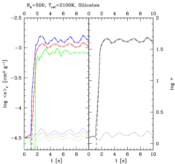
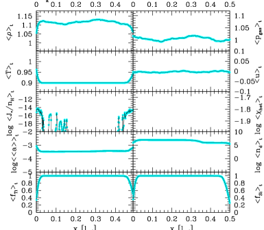
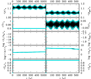
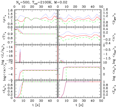
Left: Time evolution of the space means. Right: Time means as function of site over $10^{7}$ time steps.

3.1 Short term evolution

An inviscid, astrophysical test fluid in 1D with $T_{\rm ref}=2100$ K and $M=0.1$ ($\nearrow$ entree A Table 3) is excited in the wavenumber interval $[k_{\rm min},k_{\rm max}]$ by 500 modes, i. e. $N_{k}=500$, and its short term evolution is demonstrated (Figs. 1, 2; l.h.s.). The smallest eddy has than a size of $\lambda^{\rm 1D}_{\rm min}=1$ m. The simulations assume a 1D test volume in horizontal direction and gravity does therefore not influence our 1D results.

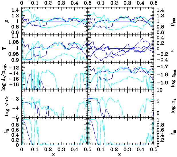
Spatial evolution:

Stochastically created waves move into the 1D test volume from both sides ($t=0.48$ s, Fig. 1) with a maximum velocity amplitude of $\cal{O}$$(10^{3}\mbox{cm \,s${}^{-1}$})$ representing the turbulent velocity fluctuations. At some instant of time, the temperature disturbance due to inward moving superimposed waves is large enough that the nucleation threshold temperature is crossed locally ($T<T_{S}$, Paper I below Eq. (21); $t=0.68$ s Fig. 1, grey/cyan solid line). As the temperature disturbance penetrates into the test volume, a nucleation front forms which moves into the dust free gas of the test volume and leaves behind dust seeds which can grow to considerable sizes (compare the change of $\log n_{d}$ from $t=0.68$ s (grey/cyan solid) and $t=1.12$ s (black dash-dot ) between $x=0$ and $x=0.16$ Fig. 1).

The superimposed waves which enter the test volume through its boundaries will also interact with each other after some time. An event-like nucleation results ($t=1.12$ s, $x=0.14$ Fig. 1). More dust is formed and meanwhile, the particles are large enough to re-initiate nucleation by efficient radiative cooling due to the strongly increased opacity ($t=1.5$ s Fig. 1, grey/cyan dash-dot).

The result is a very inhomogeneously fluctuating distribution in size, number and degree of condensation of dust in the test volume when the dust formation dominated the dynamics of the system. The fluctuations are stronger in the beginning of the simulations and homogenise with time (Fig. 2 l.h.s.). The long term behaviour will be discussed in Sect. 3.2.

Time evolution:

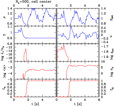
For better understanding of the time evolution of the hydrodynamic and dust quantities in a stochastically excited medium, the time evolution in the test volume’s centre (cell centre) is depicted in Fig. 2 (l.h.s) for the first 6s of the reference simulation with $N_{k}=500$.

The dust complex reaches a steady state after about $t\approx 1.8$ s in the centre of the test volume in the present simulation, for which only one singular nucleation event has been responsible (3rd panel, Figs. 2 l.h.s.). Consequently, $f_{\rm Ti}=f_{\rm Si}=1$. In contrast, the hydro- and thermodynamic quantities (gas density, $\rho$, gas pressure, $p$, and velocity, $u$) continue to fluctuate considerably around their initially homogeneous values. The small variations of the mean particle size $\langle a\rangle$ and the number of dust particles $n_{\rm d}$ are partly caused by the hydrodynamic motion in and out of the cell centre of the dust forming material and partly by the turbulent fluctuations themselves. The thermodynamic behaviour of the dust changes from adiabatic to isotherm as result of the strong radiative cooling by the dust. Therefore, the temperature drops and reaches the radiative equilibrium level ($T=T_{\rm RE}$). Exactly the same qualitative behaviour was observed from Fig. 3 in Paper I.

We conclude a different distribution of dust inside an initially dust free gas element: While in the centre of a gas element the dust formation process is completed ($f=1$) after it was initiated by waves which are emitted by its surrounding, disturbances from the boundary prevent the boundary layers of the gas elements to reach $f=1$. Consequently, a convectively ascending initially dust free cloud can be excited to form dust by waves running through it. Therefore, a cloud can be fully condensed much earlier than by any classical, static model predicted.

3.2 Long term evolution

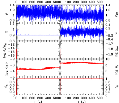
The long term behaviour of our dust forming system sets in after the dust formation process is complete ($f=1$) and radiative equilibrium ($T=T_{\rm RE}$) is reached. Due to the strong cooling capability of the dust, only small deviations occur from the radiative equilibrium if compression waves occur which may be seen as colliding small-scale turbulence elements. The general change of the temperature $T\rightarrow T_{\rm RE}$ caused an increase of the density in the test volume (density level $\rho>1$ Fig. 2 r.h.s.) in order to maintain pressure equilibrium (pressure level at $p\approx 1$, Fig. 2 r.h.s.).

The long term behaviour of $\rho$, $p$, and $u$ are characterised by strong fluctuations constantly generated by our turbulence driving. In Fig. 2 (l.h.s), which depicts a higher time resolution of Fig. 2 (r.h.s.), single waves (turbulence elements) are still distinguishable of which only spikes out of a jungle of noise are left to observe in the long term behaviour in Fig. 2 (r.h.s.).

Comparable small fluctuations of the mean particles size, $\langle a\rangle$, and the number of dust particles, $n_{d}$, occur over a long time. We recover here the 20% fluctuation which was already observable in Fig. 2 (l.h.s). Since the dust formation process is complete, these fluctuations must be of hydrodynamic origin, i. e. caused by the movement of the small-scale turbulence elements.

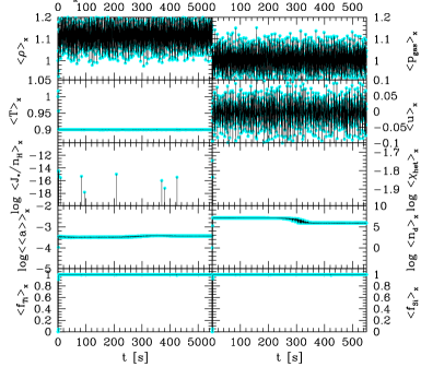
3.3 The mean behaviour in space and time

The mean behaviour of a turbulent, dust forming gas is studied. The space mean is the average over the test volume at each time step

$$\langle\alpha\rangle_{x}(t)=\frac{1}{N_{x}}\sum_{i=0}^{N_{x}}\alpha_{i}(x_{i},t)$$ (17)

and the time mean is the mean of each mesh cells over time,

$$\langle\alpha\rangle_{t}(x)=\frac{1}{N_{t}}\sum_{i=0}^{N_{t}}\alpha_{i}(x,t_{i}).$$ (18)

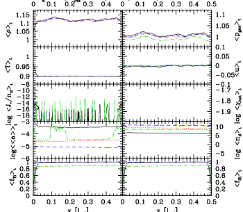
Both represent the most plausible values of the quantity $\alpha(x,t)$ i) at a certain instant of time (Eq. 17), and ii) at a certain site in the test volume (Eq. 18). The space means are calculated by leaving out the cells close to the boundary in order to exclude the fluctuations in the dust quantities due to inflowing dust-free material. Figure 3 (l.h.s.) depicts the space means $\langle\,\cdot\,\rangle_{\rm x}$ as function of time $t$ [s], and Fig. 3 (r.h.s.) depicts the time means $\langle\,\cdot\,\rangle_{\rm t}$ as function of $x$ space [$l_{\rm ref}$].

Figures 3 shows that the space and the time mean values differ considerably for the hydrodynamic quantities: Strong fluctuations of the space means (l.h.s.) occur as function of time while the time means (r.h.s.) exhibit comparatively smooth variation. These fluctuations increase with increasing number of excitation modes which shows that the fluctuations are of hydrodynamic origin (see also Sect. 3.3.1).

Figure 4: Same like Fig. 3 (l.h.s.) but $N_{k}=100$.

Space means:

The study of the long-term behaviour of the space means (l.h.s., Figs. 3) discloses a considerable variation of the hydrodynamic mean quantities. In contrast, the dust quantities are almost constant in time after the dust formation process is completed. This result is a consequence of the assumed symmetry (1D), where every wave has to cross the whole test volume which is not the case in a multi-dimensional fluid field (compare Sect. 3.5).

The formation of dust causes the temperature to change considerably towards the radiation equilibrium level causing thus the density level to change (e. g. increase if $T$ decreases) in order to recover the pressure equilibrium. Therefore, initially small perturbations in a dust forming system have a large effect on its overall hydrodynamic structure.

The strong variation of the dust quantities during the beginning of the simulation is smeared out with increasing averaging time. Therefore, observing a spatially unresolved dust forming system over a long time will not unhide the inhomogeneous behaviour though it will have a profound influence of the large-scale structure of any dust forming system, e.g., by the transition adiabatic $\rightarrow$ isothermal behaviour, by backwarming in an substellar atmosphere, or by the enrichment and the depletion by gravitational settling.

Time means:

The variation of the hydrodynamic mean values is less strong in space (r.h.s., Figs. 3) than in time (l.h.s., Figs. 3) and resembles more common expectations for such average quantities than the hydrodynamic space means do. The density shift $\rho(t=0)\,\rightarrow\,\rho(t(T=T_{\rm RE}))$ due to $T\,\rightarrow\,T_{\rm RE}$ is easier observable than for the space mean.

The time mean of the nucleation rate, however, discloses the appearance of nucleation fronts and nucleation events: Waves which enter the test volume and already carry a temperature disturbance with $T<T_{S}$ result in a nucleation front (e. g. $x\lesssim 0.025\,l_{\rm ref}$ r.h.s., Figs. 3). Waves, i. e. turbulence elements, which interact inside the test volume and only there create $T<T_{S}$ for a short time result in nucleation events as the peak like $\langle J_{*}\rangle_{t}$ shows.

Else, the dust quantities are constant in almost the whole test volume which is in agreement with their time averages. Deviations from these almost constant values occur only near the volume’s boundaries since here fresh, uncondensed material enters.

Viewing our test volume again as mass element in a convective environment which is constantly disturbed by wave propagation, we conclude that nucleation will take place everywhere in the mass element but likely with very much different efficiency. Since fresh, uncondensed material enters the mass element through open boundaries, nucleation can go on here only if the temperature is low enough. This does not cause the boundary region to contain the largest amount of dust since the dust can also leave the mass element if the fluid flow moves outward.

Figure 5: The space-means $\langle\alpha(t)\rangle_{x}$ (solid/red) with the apparent standard deviations $\sigma_{\rm N_{x}-1}^{\alpha}(t)$ (dotted/dashed) as function of time for $T_{\rm ref}=2100$  (A, l.h.s.), and $T_{\rm ref}=1900$  (C, r.h.s.); see Table 3. ($\langle\alpha(t)\rangle_{x}+\sigma_{\rm N_{x}-1}^{\alpha}(t)$ - dotted/blue; $\langle\alpha(t)\rangle_{x}-\sigma_{\rm N_{x}-1}^{\alpha}(t)$ - dashed/green).

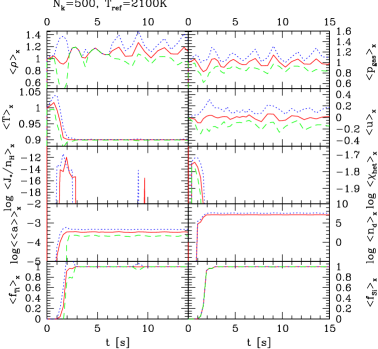
3.3.1 Dependence on the number of modes

Figure 4 depicts the same calculation like Figs. 1 – 3 but carried out with different a number of modes, $N_{k}=100$. Comparing with the l.h.s. of Fig. 3 ($N_{k}=500$) shows that the variations in the hydrodynamic quantities are smaller but the dust quantities reach very alike mean values independent of $N_{k}$.

Note, more energy is contained in the small wavenumbers (= large spatial scales) since the Kolmogoroff spectrum is applied to calculate the velocity disturbances in the Fourier space. Consequently, if a number of chosen modes, $N^{1}_{\rm k}$, is small, the smallest wavenumber will contain less energy than the smallest wavenumber for some larger number of modes $N^{2}_{\rm k}$, and, from $N^{1}_{\rm k}<N^{2}_{\rm k}$ follows $E(k_{1}({\rm N^{1}_{k}}))<E(k_{1}({\rm N^{2}_{k}}))$. This results in the appearance of larger velocity and pressure peaks with increasing $N_{\rm k}$ according to Eqs. (5) and (14).

The study of the long term behaviour of the $T_{\rm ref}=2100\,$K simulation reveals the occurrence of a long term pattern in $\rho$, $p$, and $u$ (beat frequency oscillations) with a frequency $\nu_{\rm beat}\approx 100$ s $\approx 1.7$ min. Comparing $\rho$, $p$, and $u$ in Figures 4 exhibits 6 maxima at $t\approx 50$s, 150s, 250s, 350s, 450s, 550s. This beat frequency $\nu_{\rm beat}$ seems independent on the number of modes $N_{k}$ but does, however, not establish for an excitation with a very small number of modes (e. g. $N_{k}=5$, not depicted here) and is smeared for a very large number of modes due to larger fluctuations around the mean values ($N_{k}=500$, Fig. 3).

Figure 6: Same like Fig. 5 (r.h.s.) but $M=0.02$ ($\nearrow$ entree B Table 3)

3.3.2 Apparent standard deviation

Deviations from the most plausible values, the mean values, can be studied in terms of the apparent standard deviation. The apparent standard deviation allows to estimate the mean deviations of characteristic dust quantities due to the turbulent fluid field,

$$\sigma_{N_{x}-1}^{\alpha}(t):=\sqrt{\frac{\sum_{0}^{N_{x}}(\alpha_{i}(t))^{2}-(\sum_{0}^{N_{x}}\alpha_{i}(t))^{2}/N_{x}}{N_{x}-1}}.$$ (19)

Equation (19) is therefore the mean, quadratic weighted deviation of the realisations $i$ ($i=0\ldots N_{x}$) of the turbulent, dust forming gas flow in space at an instant of time $t$. Figure 5 depicts the space means (solid) $\langle\alpha\rangle_{x}(t)$, and the respective apparent standard deviations leading to $\langle\alpha\rangle_{x}(t)+\sigma_{\rm N_{t}-1}^{\alpha}(t)$ (dotted) and $\langle\alpha\rangle_{x}(t)-\sigma_{\rm N_{t}-1}^{\alpha}(t)$ (dashed). Note that there is no straight forward functional dependence among all the lower (dashed) and all the upper (dotted) curves, respectively.

Figure 5 shows that the standard deviation is largest in the period of most active dust formation, i. e. between 0.05 s and 3 s for the Mach number case depicted (compare paragr. “Dependence on Mach number”), independent on the initial reference temperature. For example, the minimum and the maximum deviations in density deviate by almost a factor 3 for the model with $T_{\rm ref}=2100$ K ($\nearrow$ entree A in Table 3). The apparent standard deviation of the velocity field shows that $\delta u(x,t)=\pm 0.2v_{\rm ref}$ and less which is subsonic (compare Figs. 5, 6, 7) and in agreement with Ludwig et al. (2002).

The apparent standard deviations indicate that there are no very large deviations in the 1D dust quantities if the dust complex has reached it steady state, in contrast to the hydrodynamic quantities. Turbulent fluctuations will cause the dust formation to set in somewhat earlier and to occur somewhat more vivid (larger $J_{*}$). On the contrary, Figs. 5 and 6 illustrates that no dust forms if the fluctuations result in $T>T_{S}$ (no dashed line for $J_{*}$).

Dependence on temperature:

The standard deviations of the hydrodynamic quantities are not considerably larger neither in a deeper nor in a shallower turbulence excited atmospheric layer (r.h.s. Fig. 5). In contrast, the variations in the dust quantities decrease with decreasing $T_{\rm ref}$ and increase with increasing $T_{\rm ref}$ (the latter is not shown here). The nucleation rate decreases by orders of magnitude with increasing temperature and the standard deviation is considerably larger. Consequently, the mean number of dust particle is smaller and therefore the mean particle size larger. In contrast, nucleation occurs earlier and more vivid with decreasing temperature. The dust formation process is complete already during the very first time of the simulation as e. g. depicted on the r.h.s. in Fig. 5, therefore $J_{*}$ and $\chi_{\rm het}$ are not resolved on the time interval plotted. Consequently, the number of dust particles is order of magnitudes higher and the mean particles size has decreased since the material has to be distributed over a larger grain surface area than if less particles form. All of it is in accordance with common expectations (see Sect. 3.4).

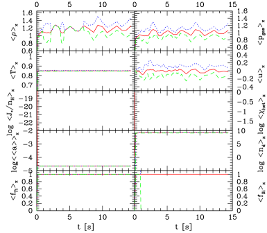
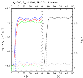
Dependence on Mach number:

Figure 6 shows a simulation comparable to the r.h.s. of Fig. 5 but now with $M=0.02$ instead of $M=0.1$ ($\nearrow$ entrees A, B in Table 3). Consequently, the characteristic time scale is much longer, namely $t_{\rm ref}\approx 15\,$s instead of $t_{\rm ref}\approx 3\,$s and a much longer time interval needs to be depicted in Fig. 6 compared to Fig. 5 in order to observe the inset of the dust formation.

We observe that the variation of the hydrodynamic quantities does not change remarkable compared to higher Mach number cases. It only appears on a much longer time scale. However, the superimposed waves need about 3 times longer to initiate the first dust formation. The nucleation is somewhat less efficient resulting in a slightly lower number of dust particles which are, hence, slightly larger. Also the growth process is less efficient compared to the M=0.1–case

Although the dust complex acts on its own, chemical time scales, it needs much longer time to reach a steady state situation if the initial Mach number is small (see also Fig. 9 in Sect. 4.1).

Figure 7: Time-means over $\approx 10$min for different temperatures $T_{\rm ref}$: dash-dot (green) - 2500K, solid (black) - 2100K (reference results), dotted (red) - 1900K, dashed (blue) - 1500K (for details on reference values see Table 1)

3.4 The dust formation window

Stochastic fluctuation can drive a reactive gas flow into the dust formation window, i. e. the thermodynamic regime where the gas - solid (or liquid) phase transition is possible and most efficient (see e. g. Sedlmayr 1997).

Depending on the thermodynamic (TD) situation, three regimes (compare Fig. 11) appear to be present in a turbulent atmosphere: The deterministic (or subcritic) contains those TD states where dust formation occurs without the need of an (e. g. hydrodynamic) ignition, i.e. the local temperature is already smaller than the nucleation threshold temperature.

The stochastic regime contains those TD states for which the dust is possible if some realistic ignition mechanism can cause $T<T_{\rm s}$. This regime contains the critical range where a transition from $T>T_{\rm s}$ to $T<T_{\rm s}$ is possible. The size of the stochastic regime depends on the turbulent energy.

The third regime can be called impossible since no dust formation would be possible here.

Temperature dependence:

We have investigated the transition deterministic – stochastic regime by studying the temperature dependence in our stochastic 1D simulations. The time mean values (Fig. 7) of the dimensionless hydrodynamic variables are very much alike ($\langle\rho\rangle_{t}$, $\langle p\rangle_{t}$, $\langle T\rangle_{t}$, $\langle u\rangle_{t}$, for reference values see Table 1) but the dust quantities deviate considerably between these two extreme regimes.

Figure 7 depicts four cases of which $T_{\rm ref}=1900,1500$K (dotted, dashed) fall into the deterministic regime in which the dust formation process is complete after a very short time on the whole test volume ($f_{\rm Ti}=f_{\rm Si}=1$) without any external excitation necessary. The $T_{\rm ref}=2500,2100$K (dash-dot, solid) fall into the stochastic regime where turbulence initiates the dust formation process by causing the very first nucleation event to occur (compare also Sect. 1). In $T_{\rm ref}=2100$K-case the dust formation process is still completed after a very short time ($t\approx 0.07$s) in the whole test volume while for $T_{\rm ref}=2500$K the first efficient nucleation event occurs only after about $65$ s $\approx 1$min. The dust formation is not complete ($f_{\rm Ti},f_{\rm Si}<1$) in this comparably hot case and even much more refined in time and space: The time mean of the mean particle size,$\langle\langle a\rangle\rangle_{t}$, varies by $\approx 1$ order of magnitude (4th panel, l.h.s, Fig. 7). Therefore, $T_{\rm ref}=2500\,$K falls in the very end of the stochastic regime being close to impossible.

$\log\,n_{\rm d}$ [cm-3] and vorticity $(\nabla\times\boldsymbol{v})$ [s-1]	$\log\langle a\rangle$ [cm]
$\log\,n_{\rm d}$ [cm-3]	$\log\langle a\rangle$ [cm]
$\log\,n_{\rm d}$ [cm-3]	$\log\langle a\rangle$ [cm]

Figure 8: 2D simulations with $T_{\rm ref}=2100$ K, $M=1$, $N_{\rm k}=500(\,\,\nearrow\,\,$entree A^′ Table 3) for three instants of time during the period of active dust formation (top: 0.8s, middle: 1.7s, bottom: 8s; $N_{\rm x}\times N_{\rm y}=128\times 128=500\,\mbox{m}\times 500\,$m, $\boldsymbol{g}=\{0,-g,0\}$)

Left: number of dust particle $\log\,$n${}_{\rm d}\,$ [cm^-3] and vorticity $(\nabla\times\boldsymbol{v}$) [s^-1] only for $t=0.8$s; Right: mean particle radius $\log\,\langle a\rangle$  [cm].

Table 1: $\rho_{\rm ref}=3.16\,10^{-4}$ g cm^-3, $l_{\rm ref}=0.5\,10^{-5}$cm

$T_{\rm ref}$	$p_{\rm ref}$	$u_{\rm ref}$	$t_{\rm ref}$	$T_{\rm RE}$
$[$K$]$	[dyn cm-2]	[cm s-1]	[s]	$[$K$]$
2500	$2.84\,10^{7}$	$3.54\,10^{4}$	2.821	1750 $(=0.7\,T_{\rm ref})$
2100	$2.38\,10^{7}$	$3.25\,10^{4}$	3.078	1890 $(=0.9\,T_{\rm ref})$
1900	$2.16\,10^{7}$	$3.09\,10^{4}$	3.236	1710 $(=0.9\,T_{\rm ref})$
1500	$1.70\,10^{7}$	$2.74\,10^{4}$	3.642	1350 $(=0.9\,T_{\rm ref})$

The temperature sequence depicted in Fig. 7 displays the transition from the deterministic into the stochastic regime: the dust formation is most efficient at the smallest temperature considered (1500K) resulting in the most dust particles (3rd panel, r.h.s., Fig. 7) and therefore in the smallest grain size. With increasing temperature, less particles are formed which can accumulate considerably more material and grow therefore to largest sizes. The hottest case considered seem not to fit into this picture because e. g. $\langle\langle a\rangle\rangle_{t,2500K}>\langle\langle a\rangle\rangle_{t,1500K}$ but $\langle\langle a\rangle\rangle_{t,2500K}\approx\langle\langle a\rangle\rangle_{t,1900K}$. Comparing the radiative equilibrium temperature of our test calculations (Table 1) indicates that $T_{\rm RE,2500K}\approx T_{\rm RE,1900K}$. Apart from the fact that considerably more time is needed to form and grow the first, initiating seed particles the higher the temperature is, the dust will drive the system locally towards this low radiative equilibrium temperature providing thereby TD conditions comparable to the $T=1900$K-case. The resultant dust quantities need therefore be comparable if $T=T_{\rm RE}$, i. e. if the gas has reached the same isothermal state.

Figure 9: Space mean and standard deviations (solid) of the total grey absorption coefficient $\kappa=\kappa_{\rm gas}+\kappa_{\rm dust}$ and the total grey optical depth $\tau$ for the simulations depicted in Fig. 5. The dust (dashed) and the gas (dotted) contributions are shown for simulations with $T_{\rm ref}=2100$ K with $M=0.1$ (l.h.s.; entree A Table 3) and with $M=0.02$ (r.h.s.; entree B Table 3).

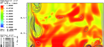
3.5 2D results

So far, only 1D results have been presented in this paper, which provide a good possibility to study the most important ongoing physical and chemical processes and their interactions. In 1D, however, each wave crosses the whole test volume and will therewith influence the local thermodynamic conditions everywhere inside the volume. In 2D, the influence of waves leads to much more complicated patterns since e. g. a non-zero rotation of the fluid field can develop. The expected consequence is a much more heterogeneous distribution of dust than in any 1D situation as it is illustrated in the following.

A 2D model calculation with $T_{\rm ref}=2100$ K, $M=1$, $N_{\rm k}$=500 ($\,\,\nearrow\,\,$ entree A^′ in Table 3) was performed on a spatial grid of $N_{\rm x}\times N_{\rm y}=128\times 128$ cells corresponding to a box of 500m $\times$ 500m. The smallest eddies have a size of $\lambda^{\rm 2D}_{\rm min}=5\,$m, the largest are of the size of the test volume. The gravity acts in negative $y$-direction, i. e. $\boldsymbol{g}=\{0,-g,0\}$. The initially homogeneous and dust free fluid is constantly disturbed by superimposed waves entering from the left, the right, and the bottom side. Thereby, a gas element is modelled which is continuously disturbed by waves originating from the surrounding convectively instable atmospheric fluid. The top side is kept open simulating the open upper boundary of a test volume in the substellar atmosphere.

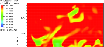
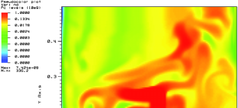
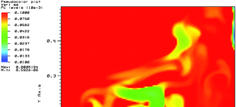
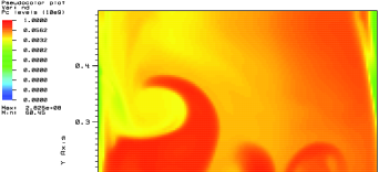
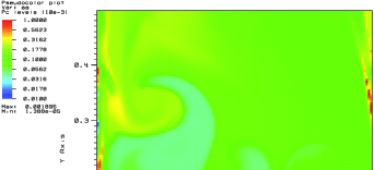
Figure 8 shows three instants of time during the phase of vivid dust formation and demonstrates the appearance of large and small dusty scale structures evolving with time. Both, the number of dust particles $n_{\rm d}$ (l.h.s.) and the mean particle size $\langle a\rangle$ (r.h.s.), are plotted on a logarithmic scale with $n_{\rm d}=1\,\ldots\,10^{9}$ cm^-3 and $\langle a\rangle=10^{-5.5}\,\ldots\,10^{-3.5}$. The very inhomogeneous appearance of the dust complex is a result of nucleation fronts and nucleation events comparable to our 1D results. The nucleation is now triggered by the interaction of eddies coming from different directions. Large amounts of dust are formed and appear to be present in lane-like structures (large $\log\,$n_d; dark areas). The lanes are shaped by the constantly inward travelling waves. Our simulations show that some of the small-scale structure merge thereby supporting the formation of lanes and later on even larger structures. The formation of such large structures is not caused by the establishment of a pressure gradient to counterbalance the gravity. Since the whole test volume is only of the size of $H_{\rm P}/20$ the resulting pressure gradient is negligibly small. Hence, the large-scale structures result from the interaction of dust formation and turbulence.

Furthermore, dust is also present in curl-like structure which indicates the formation of vortices. As the time proceeds in our 2D simulation, vortices develop orthogonal to the velocity field which show a higher vorticity ($\nabla\times\boldsymbol{v}(\boldsymbol{x},t)$) than the majority of the background fluid field. For illustration, the maximum and the minimum vorticity between $\approx-20$ s^-1 and $\approx 20$ s^-1 has been superimposed as a contour plot (grey/black) on top of the false colour plot of the number of dust particles for $t=0.8$ s in Fig. 8 (l.h.s., top). This shows that the vortices with high vorticity preferentially occur in dust free regions or regions with only little amounts of dust present. The motion of the vortices can transport the dust particles into region with still condensible material available, and seem thereby to cause larger and larger dusty areas to form.

The 2D hydrodynamic behaviour is comparable to our 1D results in the sense that the stochastically created waves enter the test volume, interact, run through the test volume, and eventually leave it at the top side after they have initiated the dust formation process. Large changes in the dust quantities during short time intervals occur locally during the time period of the first nucleation and the re-initiation of nucleation by radiative cooling. A spatially inhomogeneous dust distribution results which is only slightly shifted back and forth by the inward moving superimposed waves. In contrast, considerable variations in $\rho$, $p$, and in the velocity components $(u,v)$ occur in time and space. Furthermore, a new qualitative behaviour compared to the 1D simulation appears. Hydrodynamic advection gathers the dust in larger and larger structures while the formation of the dust has been initiated in the small-scale regime of the simulation. The reference time of our present 2D simulation is comparably high (see Table 3). We have, however, done 1D test calculations (Figs. 5, 6, 9) which indicate that in the low Mach number case the global dust formation time scale (i. e. the time when the dust formation reaches its steady state) will merely increase (for discussion see Sect. 4.2).

4 Discussion

4.1 Variability

Observational evidence has been provided (Bailer-Jones & Mund 1999, 2001a,b; Martín et al. 2001; Gelino et al. 2002; Clarke et al. 2002) that Brown L-Dwarfs are non-periodically photometric variable at a low level of $1-2\%$ (Clarke 2002) and sometimes even larger. Nakajima et al (2000) and Kirkpatrick et al. (2001) reported on spectroscopic variability. Appealing explanations are the appearance of magnetic spots or the formation of dust clouds. Mohanty et al. (2002) and Gelino et al. (2002) have argued that ultra cool dwarfs are unlikely to support magnetic spots. There is, however, evidence for magnetic activity in L dwarfs by a rapid declining, strong H$\alpha$ emission. In contrast, three objects are observed with a persistent, strong H$\alpha$ emission (Liebert${\rm\hskip 3.44444ptet\hskip 3.01385ptal.\hskip 2.15277pt}$ 2003). A straight forward, consistent explanation is not at hand yet and will probably be theoretically very demanding. We, therefore, follow in this paper the hypothesis of the formation of dust clouds in a convectively influenced turbulent environment as explanation of non-periodic variability

Ludwig et al. (2002) argue based on their hydrodynamic 3D simulation that M-dwarfs (and even more Brown Dwarfs) show only very little temporal and horizontal fluctuations in their atmospheres. Dust strongly interacts with the thermo- and hydrodynamics due to radiative transfer effects, gas phase depletion and on macroscopic scales due to drift. It seems therefore likely to expect a support of initially small inhomogeneouties by these processes. Woitke (2001) has carried out 2D radiative transfer calculations for a inhomogeneous density distribution which support this idea. Since the radiation is blocked by condensing dust clouds of sufficient optical depth, the radiation is forced to escape mainly through the remaining wholes, thereby enhancing and preventing the dust formation, respectively.

One may speculate that the consideration of dust formation in 3D simulation may even cause these models to deviate considerably from the simple MLT models in the case of brown dwarfs due to the time dependence of the dust formation process and the corresponding feedback on the space and time evolution.

Optical depth:

Figure 9 (left panels) depicts the space mean total opacity (solid lines) and the mean opacity of the dust (dashed lines) and the gas (dotted lines) for the 1D test calculation investigated in Fig. 7. Upper curves indicate $\langle\kappa\rangle_{x}(t)+\sigma_{\rm N_{t}-1}^{\kappa}(t)$, the lower depict $\langle\kappa\rangle_{x}(t)-\sigma_{\rm N_{t}-1}^{\kappa}(t)$. The Rosseland mean dust opacities for astronomical silicates ($\kappa_{\rm dust}=0.75\,\rho L_{3}1.74\,T^{1.12}$, Paper I; l.h.s.) and a typical Rosseland gas mean of $\kappa_{\rm gas}=0.1$ g/cm³ have been adopted. The Rosseland gas mean opacity was chosen typical for a hot, inner layer of a brown dwarf atmosphere. Figure 9 shows that the dust and the gas opacities differ by about 1.5 orders of magnitude. The dust opacities varies by about 0.5 magnitudes, the gas opacity by only about 0.2 order of magnitudes. this is independent of the characteristic time scale of the system, i. e. the large-scale Mach number of the initial configuration (compare l.h.s. and r.h.s. in Fig. 9).

Figure 9 further depicts in the right panels the time evolution of the space mean of the optical depth which a mass element of the size of our test volume (500 m) would have. The optical depth increases by a factor of 10 when the dust forms in accordance with the opacity increase. There is, however, a delay between the inset of dust formation and the time when the maximum optical depth is reached because the dust formation sets in earlier than a cloud becomes optically thick. This delay is sensitive to the characteristic time scale of the system as a comparison of the l.h.s. and r.h.s. in Fig. 9 demonstrate.

The gas/dust mixture will only be optically thick in the case of non-transparent dust particles (e. g. astronomical silicates) which may depend on the wavelength considered. Glassy grains may efficiently absorb in the far IR ($\lambda\ga 10\mu$m) and one might, depending on the observed wavelength, detect typical dust features and possibly even the rapid formation events which, however, may need to evolve on macroscopic scales in order to be observable.

Turbulent fluctuation seem not to produce considerable variations in view of the space mean of the optical depth in the long term (here $t>4$ s) if astronomical silicates are assumed as typical dust opacity carriers.

4.2 Towards the observable regime

The time-dependent simulations performed so far might suggest an up-scaling of the achieved results in order to estimate e.g. possible cloud sizes and variability time scales on an observational level. This idea is not as straight forward as it might seem because of the differences between chemical and hydrodynamical time scales. Dust formation is a local process and its (local) time scale is the same independent of the hydrodynamical regime but the hydrodynamic time scale changes depending on e. g. the characteristic length of the regime considered. A simple and correct up-scaling according to the principle of similarity would require the characteristic numbers to remain the same which is not the case (see also Helling 2003, Lingnau 2004), for instance due to the changing characteristic hydrodynamic time scales. One might further imagine to upscale the results by a periodic continuation, i.e. each small-scale simulation being one pixel of the large-scale picture. In any case, the feedback of the large scale (e.g. convective) motions on the small scales is neglected and visa versa. Important effects like chemical mixing and kinetic energy input into the turbulent fluid field are than missing. Consequently, the non-linear coupling between dust formation and hydrodynamics makes it impossible to simply scale up detailed small-scale results into an regime accessible by observations. The complete large-scale simulation needs to be awaited.

The aim of the investigations of the small-scale regimes performed so far was indeed to provide information and understanding for building a large-scale model of a brown dwarf atmosphere. From these results, we suggest the following necessary criteria for a sub-grid model (also called closure term or closure approximation) of a turbulent, dust forming system:

• A sub-grid model must describe the transition deterministic $\rightarrow$ stochastic dust formation, depending on the turbulent energy as e. g. measured by the large-scale variations of the local velocity field.

• The dust formation process (nucleation + growth) is restricted to a short time interval (of the order of a few seconds), which is usually much smaller than the large-scale hydrodynamic time scale. This involves that:

  • The nucleation occurs locally and event-like in very narrow time slots.

  • The growth process continues as long as condensible material is available and thermal stability of the dust is assured.

  • The condensation process finally freezes in and the inhomogeneous dust properties are preserved.

• The dust formation process should be accompanied by a fast transition from an approximately adiabatic to an approximately isothermal behaviour of the dust/gas mixture. This transition can be expected to affect the convective stability in substellar atmospheres.

4.3 Comparison with classical model atmospheres

Figure 10: The deterministic and the stochastic dust formation regime in comparison to typical substellar model atmospheres (solar metalicity, $\log g=5$, AH (black) = Allard${\rm\hskip 3.44444ptet\hskip 3.01385ptal.\hskip 2.15277pt}$2001, T (grey/cyan) = Tsuji 2002).
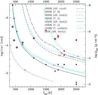
(open circles (black) - dust formation without ignition; asterisk (blue) - dust growth on initially present seed particles (1cm^-3); squares (red) - dust formation under turbulent conditions; triangles (black) - $(T_{\rm ref},\rho)$ pairs investigated; hooks - border of convective zone)

Figure 10 revisits the idea of the dust formation window but now with view on classical brown dwarf atmosphere calculations.

The following calculations are performed for various $(T,\rho)$ pairs in order to demonstrate in which atmospheric regions dust formation will simply take place (deterministic regime) and in which regions dust formation needs to be initiated (stochastic regime; compare Sect. 3.4). For eye guidance, the $(T,\rho)$ pairs are indicated by small black triangles along with presently used substellar model atmospheres in the literature (Allard${\rm\hskip 3.44444ptet\hskip 3.01385ptal.\hskip 2.15277pt}$2001 – black lines, Tsuji 2002 – grey/cyan lines). One may notice that the warm models of the same stellar parameter can differ by about 500 K for a given density in the inner atmospheric region which is convectively unstable in both cases. Small hooks (red) indicate the upper Schwarzschild boundary (SB) for convection if available, i. e. $v_{\rm MLT}=0$ for $T<T_{\rm SB}$. The test is simple: Two calculations are carried our for each $(T,\rho)$ pair where in the first test a small number of seed particles is prescribed ($\rho L_{0}=1$cm^-3; open black circles), and in the second test no seed particles are prescribed (blue asterisks). The results should be almost identical inside the deterministic regime but no dust should form in the stochastic regime.

One observes that there is no difference in grain size in the cool outer atmospheric region whether seed particles are initially present or not. The initially present little number of seed particles is overran by a very efficient nucleation which is characteristic for the deterministic regime. Note that the dust grains will immediately start to move inwards on macroscopic scales of atmospheric extension due to the large gravity of brown dwarfs. However, depending on the TD conditions, the nucleation efficiency varies in the atmosphere. The more efficient nucleation takes place, the more seed particles are formed resulting in smaller mean sizes because the gaseous material has to be distributed over more particles than in case of less efficient nucleation. Small mean particle sizes inside the deterministic regime are therefore a sign for efficient dust nucleation.

For $T>1800$ K, the stochastic regime is entered. Here, dust is only present if by some mean a certain number of seeds is present (blue asterisks) or a ignition mechanism (e. g. turbulence, radiative cooling by gas) provides the appropriate TD conditions (red squares). Note that no open circles appears at this site of Fig. 10 since the TD conditions are now inappropriate for a gas - solid phase transition except an ignition mechanism is present.

5 Conclusions

We have studied the onset of the dust formation process in a turbulent fluid field, typical for the dense and initially dust-hostile regions in substellar atmospheres. The main scenario is a convectively ascending fluid element in a brown dwarf atmosphere, which is excited by turbulent motions and just reaches sufficiently low temperatures for condensation, but other applications are also conceivable. The dust formation in a turbulent gas is found to be strongly influenced by the existence of a nucleation threshold temperature $T_{S}$. The local temperature $T$ must at least temporarily decrease below this threshold in order to provide the necessary supersaturation for nucleation.

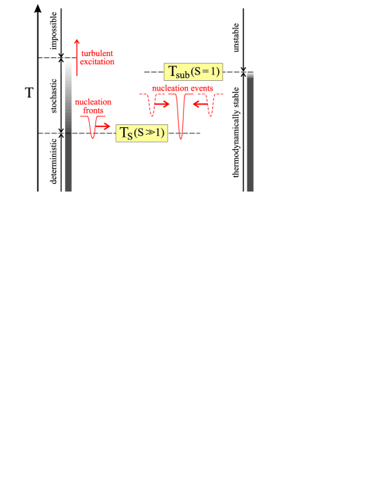
Depending on the relation between the local mean temperature $\overline{T}$ and $T_{S}$, three different regimes can be distinguished (see l.h.s. of Fig. 11): (i) the deterministic regime ($\overline{T}<T_{S}$) where dust forms anyway, (ii) the stochastic regime ($\overline{T}>T_{S}$) where $T<T_{S}$ can only be achieved locally and temporarily by turbulent temperature fluctuations, and (iii) a regime where dust formation is impossible. The size of the stochastic regime depends on the available turbulent energy. This picture of turbulent dust formation is quite different from the usually applied thermodynamical picture (r.h.s. of Fig. 11) where dust is simply assumed to be present whenever $T<T_{\rm sub}$, where $T_{\rm sub}$ is the sublimation temperature of a considered dust material.

Figure 11: Regimes of turbulent dust formation. $T_{S}$: nucleation threshold temperature (supersaturation $S\ll 1$ required), $T_{\rm sub}$: sublimation temperature.

The investigations have been performed in the mesoscopic scale regime, where the test volume is excited by a spectrum of waves within a limited $k$-interval at given energy distribution, which are generated at the boundaries (pseudo-spectral method for driven turbulence). Two basic processes are found to be capable to initiate the dust formation even in a host-hostile environment:

• expansion waves with $\overline{T}-\Delta T<T_{S}$ (nucleation fronts).

• interactions of two or more expansion waves which cannot produce sufficiently low temperatures for themselves, but the superposition of such waves can $\overline{T}-\Delta T_{1}-\Delta T_{2}-\ldots<T_{S}$ (nucleation events).

After initiation, the dust condensation process is completed by a phase of active particle growth until the condensible elements are consumed, thereby preserving the dust particle number density for long times. However, radiative cooling (as follow-up effect) is found to have an important influence on the subsequent dust formation, if the dust opacity reaches a certain critical value. This cooling leads to a decrease of $\overline{T}(t)$ which may re-initiate the nucleation. This results in a runaway process (unstable feedback loop) until radiative and phase equilibrium is achieved. Depending on the difference between the initial mean temperature $\overline{T}(t\!=\!0)$ and the radiative equilibrium temperature $T_{\rm RE}$, a considerable local temperature decrease and density increase occurs. Since the turbulent initiation of the dust formation process is time-dependent and spatially inhomogeneous, considerable spatial variations of all physical quantities (hydro-, thermodynamics, dust) occur during the short time interval of active dust formation (typically a few seconds after initiation), which actually creates new turbulence.

Thus, small turbulent perturbations have large effects in dust forming systems. A convectively ascending, initially dust free gas element, which is slightly warmer than its surroundings, can be excited to form dust by waves running through it, even at otherwise dust-hostile temperatures. The newly created dust particles may cause the substellar atmosphere to become almost instantaneously optically thick. Our 2D simulations show that the dust appears in lane-like and curled structures. Small-scale dust structures merge and form larger structures. Vortices appear to be present preferentially in regions without or with only little dust. Non of these structures would occur without turbulent excitation.

Appendix A Analysis of characteristic numbers & characteristic values of test calculations

Table 2: Characteristic numbers and reference values used to analyse the chemistry and physics in the mesoscopic scale regime. Hydro- and thermodynamic reference values have been guided by static brown dwarf model atmosphere calculations (Tsuji 2002). The reference values for the dust complex have been adopted from the experiences gained in Paper I. Considered is the TiO₂ seed formation and growth by SiO and TiO₂. ($\gamma=7/5$, $a_{\rm l}^{\rm TiO_{2}}=1.95\cdot 10^{-7}$cm, $m_{\rm H}$ mass of the hydrogen atom, $\sigma$ Stefan-Boltzmann constant, $k$ Boltzmann constant, $\mu_{\rm kin}$ kinematic viscosity [g cm^-1s^-1], $N_{l}=1000$)

Name	Characteristic		Value
	Number		inside		outside
Reynolds number	${\bf\rm Re}=\frac{v_{\rm ref}l_{\rm ref}\rho_{\rm ref}}{\mu_{\rm kin}}$
	$=5.88\cdot 10^{-6}\sqrt{T}\qquad^{(*)}$		$1.2\,10^{10}$	$\ldots$	$1.2\,10^{7}$
Mach number	${\bf\rm M}=\frac{v_{\rm ref}}{c_{\rm s}}$			0.1
Froude number	${\bf\rm Fr}=\frac{v_{\rm ref}^{2}}{l_{\rm ref}}\frac{1}{g_{\rm ref}}$		0.11		0.05
Radiation number	${\bf\rm Rd}=4\kappa_{\rm ref}\sigma T^{4}_{\rm ref}\cdot\frac{t_{\rm ref}}{P_{\rm ref}}$		$0.207$	$\ldots$	$8.6\,10^{-3}$	(◇)
			$2.07$	$\ldots$	$0.86$	(◇◇)
Damköhler number of nucleation	${\bf\rm Da^{\rm nuc}_{\rm d}}=\frac{t_{\rm ref}J_{*,{\rm ref}}}{\rho_{\rm ref}L_{0,{\rm ref}}}$		0	$\ldots$	$3.24\,10^{5}$
Damköhler number of growth	${\bf\rm Da^{\rm gr}_{\rm d}}=\frac{t_{\rm ref}\chi_{\rm ref}}{(\frac{4\,\pi}{3}\langle a\rangle^{3}_{\rm ref})^{1/3}}$		$9.78\,10^{4}$	$\ldots$	$97.8$
				$j=0$ : $1$
Sedlmaÿr number $(j\in\mathbb{N})$	${\bf\rm Se_{\rm j}}=\left(\frac{a_{l}}{\langle a\rangle_{\rm ref}}\right)^{\rm j}$			$j=1$ : $0.195$
				$j=2$ : $0.0381$
				$j=3$ : $7.44\,10^{-3}$
Element Consumption number	${\bf\rm El}=\frac{\rho_{\rm ref}L_{0,{\rm ref}}N_{l}}{n_{\rm<H>,ref}\epsilon_{\rm ref}}$			$7.27\,10^{-4}$
Name	Reference Value		Value
			inside		outside
temperature	$T_{\rm ref}$	[K]	2200	$\ldots$	1000
density	$\rho_{\rm ref}$	[g/cm3]	$10^{-3}$	$\ldots$	$10^{-6}$
thermal pressure	$P_{\rm ref}=\frac{kT_{\rm ref}\rho_{\rm ref}}{2.3m_{\rm H}}$	[dyn/cm2]	$7.78\,10^{7}$	$\ldots$	$3.54\,10^{4}$
velocity of sound	$c_{\rm S}=\sqrt{\gamma\frac{P_{\rm ref}}{\rho_{\rm ref}}}$	[cm/s]	$3.3\,10^{5}$	$\ldots$	$2.23\,10^{5}$
velocity	$v_{\rm ref}$	[cm/s]		$\approx c_{\rm S}/10$
length	$l_{\rm ref}$	[cm]		$10^{5}$
hydrodyn. time	$t_{\rm ref}=\frac{l_{\rm ref}}{v_{\rm ref}}$	[s]	$3.03$	$\ldots$	4.49
gravitational acceleration	$g_{\rm ref}$	[cm/s2]		$10^{5}$
total absorption coefficient	$\kappa_{\rm ref}$	[1/cm]	$10^{-3}$	$\ldots$	$3\cdot 10^{-7}$	(◇)
			$0.1$	$\ldots$	$3\cdot 10^{-5}$	(◇◇)
nucleation rate	$J_{*,\rm ref}/n_{\rm<H>,ref}$	[1/s]	$0$	$\ldots$	$2.5\cdot 10^{-6}$
0th dust moment ($=n_{\rm d}/\rho$)	$L_{0,\rm ref}$	[1/g]		$\ldots$	$1.35\,10^{14}$	(□)
heterog. growth velocity	$\chi_{\rm ref}$	[cm/s]	$\lesssim 0$	$\ldots$	$3.51\,10^{-5}$
mean particle radius	$\langle a\rangle_{\rm ref}$	[cm]		$10^{-6}$
element abundance	$\epsilon_{\rm ref}$	[–]		$10^{-6}$
total hydrogen density	$n_{\rm<H>,ref}=\frac{\rho_{\rm ref}}{1.4\,m_{\rm H}}$	[1/cm3]	$4.22\,10^{20}$	$\ldots$	$4.22\,10^{17}$
SiO density	$n_{\rm<SiO>,ref}$	[1/cm3]	$1.50\,10^{16}$	$\ldots$	$1.50\,10^{13}$
TiO2 density	$n_{\rm<TiO_{2}>,ref}$	[1/cm3]	$4.12\,10^{13}$	$\ldots$	$4.10\,10^{10}$

^(∗) For a H₂/He rich gas (Eq. (10) in Woitke${\rm\hskip 2.41109pt\&\hskip 2.41109pt}$Helling 2003a). ^(◇) gas only ^(◇◇) dust and gas ^(□) Gail & Sedlmayr (1999)

Table 3: Characteristic numbers and reference values for the test calculations carried out in the previous sections. For definition of characteristic numbers see Table 2

		A	B	C	A′
Hydro- & Thermodynamic
$T_{\rm ref}$	[K]	2100	2100	1900	2100
$\rho_{\rm ref}$	[g cm-3]	$3.16\,10^{-4}$	$3.16\,10^{-4}$	$8.13\,10^{-4}$	$3.16\,10^{-4}$
$l_{\rm ref}$	[cm]	$10^{5}$	$10^{5}$	$10^{5}$	$10^{5}$
$v_{\rm ref}$	[cm s-1]	$3.25\,10^{4}$	$6.50\,10^{3}$	$3.09\,10^{4}$	$3.25\,10^{5}$
$g_{\rm ref}$	[cm s-2]	$10^{5}$	$10^{5}$	$10^{5}$	$10^{5}$
$T_{\rm RE}$	[K]	$1980$ $(=0.9T_{\rm ref})$	$1980$ $(=0.9T_{\rm ref})$	$1710$ $(=0.9T_{\rm ref})$	$1980$ $(=0.9T_{\rm ref})$
$\kappa_{\rm ref}$	[1/cm]	$2\,10^{-5}$	$2\,10^{-5}$	$2\,10^{-5}$	$2\,10^{-5}$
Dust & Chemistry
$J_{\rm*,ref}$	[s-1cm-3]	$10^{12}$	$10^{12}$	$10^{12}$	$10^{12}$
$a_{\rm ref}$	[cm]	$10^{-6}$	$10^{-6}$	$10^{-6}$	$10^{-6}$
$\chi_{\rm ref}$	[cm s-1]	$10^{-2}$	$10^{-2}$	$10^{-2}$	$10^{-2}$
$L_{\rm 0,ref}$	[g-1]	$10^{10}$	$10^{10}$	$10^{10}$	$10^{10}$
Derived reference values
pref	[dyn cm-2]	$2.38\,10^{7}$	$2.38\,10^{7}$	$5.54\,10^{7}$	$2.38\,10^{7}$
tref	[s]	3.08	15.4	3.24	0.3
$L_{\rm j,ref}$	[cmjg-1]	$(\frac{4\pi\,a_{\rm ref}^{3}}{3})^{j/3}L_{\rm 0,ref}$	$(\frac{4\pi\,a_{\rm ref}^{3}}{3})^{j/3}L_{\rm 0,ref}$	$(\frac{4\pi\,a_{\rm ref}^{3}}{3})^{j/3}L_{\rm 0,ref}$	$(\frac{4\pi\,a_{\rm ref}^{3}}{3})^{j/3}L_{\rm 0,ref}$
Hydro- & Thermodynamic
$M$		1/10	1/50	1/10	1
$Fr$		0.105	$4.22\,10^{-3}$	0.095	10.5
$Rd$		$1.139\,10^{-2}$	$5.70\,10^{-2}$	$3.45\,10^{-3}$	$1.14\,10^{-3}$
Dust & Chemistry
$Da^{\rm nuc}_{\rm d}$		$9.73\,10^{5}$	$4.87\,10^{6}$	$3.98\,10^{5}$	$9.73\,10^{4}$
$Da^{\rm gr}_{\rm d}$		$1.91\,10^{4}$	$9.55\,10^{4}$	$2.01\,10^{4}$	$1.91\,10^{3}$
$Se_{0}$		1.0	1.0	1.0	1.0
$Se_{1}$		0.195	0.195	0.195	0.195
$Se_{2}$		$3.8\,10^{-2}$	$3.8\,10^{-2}$	$3.8\,10^{-2}$	$3.8\,10^{-2}$
$Se_{3}$		$7.41\,10^{-3}$	$7.41\,10^{-3}$	$7.41\,10^{-3}$	$7.41\,10^{-3}$
$El$		$1.41\,10^{-7}$	$7.07\,10^{7}$	$3.82\,10^{-7}$	$1.41\,10^{-7}$
Turbulence
$\varepsilon$ (Eq. 3)	[cm2 s-3]	$2.40\,10^{8}$	$1.92\,10^{6}$	$2.06\,10^{8}$	$2.41\,10^{11}$
$S_{\rm ref}$ (Eq. 16)	[erg/K]	$1.42\,10^{9}$	$1.37\,10^{9}$	$1.28\,10^{9}$	$1.4\,10^{9}$
$k_{\rm min}=2\pi/l_{\rm max}$	[1/cm]	$6.30\,10^{-5}$	$6.30\,10^{-5}$	$6.30\,10^{-5}$	$6.30\,10^{-5}$
$k_{\rm max}=2\pi/(3\,dx)$	[1/cm]	$2.10\,10^{-2}$	$2.10\,10^{-2}$	$2.10\,10^{-2}$	$5.30\,10^{-3}$
$l_{\rm max}$	[cm]	$l_{\rm ref}$	$l_{\rm ref}$	$l_{\rm ref}$	$l_{\rm ref}$
$dx$ for $N_{x}=500$ (1D)	[cm]	$1.00\,10^{2}$	$1.00\,10^{2}$	$1.00\,10^{2}$	$-$
$dx$ for $N_{x}=128$ (2D)	[cm]	$-$	$-$	$-$	$3.94\,10^{2}$

References

- (1) Ackermann S., Marley M., 2001, ApJ 556, 872
- (2) Allard F., Hauschildt P., Alexander D., Tamanai A., Schweitzer A., 2001, ApJ 556, 357
- (3) Bailer-Jones C. A. L., Mundt R., 1999, A&A 348, 800
- (4) Bailer-Jones C. A. L., Mundt R., 2001, A&A 374, 1071
- (5) Bailer-Jones C. A. L., Mundt R., 2001, A&A 367, 218
- (6) Botta, N., Klein, R., Langenberg, S., Lützenkirchen, S., 2003, JCP submitted
- (7) Burrows A., Marley M., Hubbard W. B., Lunine J. I., Guillot T., Saumon D., Freedman R., Sudarsky D., Sharp C., 1997, ApJ 491, 856
- (8) Canuto V. M., 1997a, ApJ 482, 827
- (9) Canuto V. M., 1997b, ApJ 478, 322
- (10) Canuto V. M., 2000, ApJ 541, L79
- (11) Caunt S., Korpi M., 2001, A&A 369, 706
- (12) Chang C., John M., Patzer A. B. C., Sedlmayr E., 1998, In Buttet J., Châtelain A., Monot R., Broyer M., Harbich W., Perez A., Reuse F., Schneider W. D., Book of Abstracts, 4.2.
- (13) Chang C., Patzer A. B. C., Sedlmayr E., , Steinke T., Sülzle D., 2001, Chem. Phys. 271, 283
- (14) Cho J.-K., Polvani L., 1996, Phys.Fluids 8, 1531
- (15) Clarke F., 2003, Variability in Ultra Cool Dwarfs, PhD thesis, Darwin College, Cambridge, GB
- (16) Cooper C. S., Sudarsky D., Milsom J. A., Lunine J. I., Burrows A., 2003, ApJ 586, 1320
- (17) Deuflhard P., 1983, Numer. Math. 41, 399
- (18) Deuflhard P., Nowak U., 1987, In Deuflhard P., Engquist B., Large Scale Scientific Computing. Progress in Scientific Computing 7, 37. Birkh user
- (19) Dominik C., Sedlmayr E., Gail H.-P., 1993, A&A 277, 578
- (20) Dubois T., Janberteau F., Teman R., 1999, Dynamic Multilevel Methods and the Numerical Simulation of Turbulence, Cambridge University Press
- (21) Ehrig E., Nowak U., Oeverdieck L., Deuflhard P., 1999, In Bungartz H.-J., Durst F., Zenger C., High Performance Scientific and Engineering Computing. Lecture Notes in Computational Science and Engineering, 233. Springer
- (22) Eswaran V., Pope S., 1988, Computers & Fluids 16(3), 257
- (23) Eswaran V., Pope S., 1988, Phys. Fluids 31(3), 506
- (24) Frisch U., 1995, Turbulence, Cambridge University Press, Cambridge
- (25) Gail H.-P., Sedlmayr E., 1986, A&A 166, 225
- (26) Gail H.-P., Sedlmayr E., 1988, A&A 206, 153
- (27) Gail H.-P., Sedlmayr E., 1998, In Sarre P., Chemistry and physics of molecules and grains in space. Faraday Discussion no. 109, 303, London, GB
- (28) Gail H.-P., Sedlmayr E., 1999, A&A 347, 594
- (29) Gail H.-P., Keller R., Sedlmayr E., 1984, A&A 133, 320
- (30) Gelino C. R., Marley M. S., 2000, In Griffith C. A., Marley M. S., From Giant Planets to Cool Stars, 322
- (31) Gelino C., Marley M., Holtzman J., Ackerman S., A, Lodders K., 2002, ApJ 577, 433
- (32) Helling Ch., Oevermann M., Lüttke M., Klein R., Sedlmayr E., 2001, A&A 376, 194
- (33) Helling Ch., 2003, Habilitationsschrift, Technische Universität Berlin
- (34) Jeong K. S., Winters J. M., Fleischer A. J., Sedlmayr E., 1998, In Guzik J. A., Bradley P. A., A Half-Century of Stellar Pulsation Interpretations: A Tribute to Arthur N. Cox, 335. ASP Conf. Ser.
- (35) Jeong K. S., Winters J. M., Sedlmayr E., 1999, In Le Bertre T., Lèbre A., Waelkens C., IAU Symp. 191: Asymptotic Giant Branch stars, 233. ASP
- (36) Jeong K. S., Chang C., Sedlmayr E., Sülzle D., 2000, J. Phys. B 33, 3417
- (37) Jeong K., Winters J., Le Bertre T., Sedlmayr E., 2003, A&A 407, 191
- (38) Jimenez J., Wray A., Saffman P., Rogallo R., 1993, JFM 255, 65
- (39) John M., 2003, Physical properties of clusters relevant for the dust formation process in oxygen-rich astrophysical environments, PhD thesis, Technische Universtät Berlin, Berlin, Germany
- (40) Kirkpatrick J., Dahn C., Monet I., D.G.and Reid, Gizis J., Liebert J., Burgasser A., 2001, AJ 6, 3235
- (41) Liebert, J., Kirkpatrick, J.D., Cruz, K.L., Reid, I.N., Burgasser, A., Tinney, C.G., Gizis, J.E.,2003, AJ 125, 343
- (42) Lingau, K., 2004, Diploma Thesis, Technische Universität Berlin
- (43) Ludwig H.-G., Allard F., Hauschildt P. H., 2002, A&A 395, 99
- (44) Martín E., Zapatero Osorio M., Lehto H., 2001, ApJ 557, 822
- (45) Menou K., Cho J.-K., Seager S., Hansen B., 2003, ApJ 587, L113
- (46) Michael B., Nuth III J., Lilleleht L., 2003, ApJ 590, 579
- (47) Mac Low M.-M., 1999, ApJ 524, 169
- (48) Mac Low M.-M., Klessen, R.H. 2004, RvMP 76, 125
- (49) Mohanty S., Basri G., Shu F., Allard F., Chabrier G., 2002, ApJ 571, 469
- (50) Nakajima T., Tsuji T., Maihara T., Iwamuro F., Motohara K., Taguchi T., Hata R., Tamura M., Yamashita T., 2000, PASJ 52, 87
- (51) Nowak U., Ehrig E., Oeverdieck L., 1998, In Sloot M., P. and Bubak, Hertzberger B., High-Performance Computing and Networking. Lecture Notes in Computer Science Vol. 1401, 419. Springer
- (52) Overholt, M.R., Pope, S.B., 1998, Computers & Fluids 27/1, 11
- (53) Patzer A. B. C., Chang C., John M., Bolick U., Sülzle D., 2002, Chem. Phys. Lett. 363, 145
- (54) Reinecke M., Hillebrandt W., Niemeyer J., 2002, A&A 386, 936
- (55) Röpke F., Niemeyer J., Hillebrandt W., 2003, ApJ 588, 952
- (56) Rossow W. V., 1978, Icarus 36, 1
- (57) Schmidt H., Klein R., 2003, Combustion Theory and Modelling, submitted
- (58) Schneider T., Botta N., Geratz K., Klein R., 1999, JCP 155, 248
- (59) Seager S., Sasselow D., 2000, ApJ 537, 916
- (60) Sedlmayr E., 1997, Ap&SS 251(1-2), 103
- (61) Smiljanovski V., Moser V., Klein R., 1997, Combustion Theory & Modelling 1, 183
- (62) Smith M. D., Mac Low M.-M., Heitsch F., 2000, ApJ 362, 333
- (63) Straka C., 2002, PhD thesis, Ruprecht-Karls-Universität Heidelberg
- (64) Tielens A., Waters L., Molster F., Justanount K., 1998, In Waters L., Waelkens C., van der Hulst K., Zaal P., ISO’s view on stellar Evolution, 415, Kluwer Academie Press, Belgium
- (65) Tsuji T., 2002, ApJ 575, 264
- (66) Tsuji T., 2002, In Jones H., Steele I., Ultracool Dwarfs: New Spectral Types L and T, 9, Springer, Berlin, Heidelberg
- (67) Wallin B. K., Watson W. D., Wyld H. W., 1998, ApJ 495, 774
- (68) Woitke P., Helling Ch., 2003, A&A 399, 297
- (69) Woitke P., Helling Ch., 2004, A&A 414, 335