Bayesian Hypothesis Testing for Planet Detection

Isabelle Braems111I. Braems received a fellowship from the Institut National de Recherche en Informatique et Automatique (INRIA) Laboratoire d’Etudes des Mat riaux Hors-Equilibre (LEMHE) N. Jeremy Kasdin Princeton University
Abstract

The past five years has seen a surge in research and innovative ideas for the imaging of extrasolar planets, particular terrestrial ones. We expect that within the next decade a space observatory will be launched with the objective of imaging earthlike planets. Because of the limited lifetime of such a mission and the large number of potential targets, integration time is a critical parameter. In fact, integration time is the primary metric in evaluating various design approaches for the high contrast imaging system. In this paper we present a new approach to determining the existence of a planet in an observed system using Bayesian hypothesis testing. Rather than perform photometry, or rely on vision to determine the existence of a planet, this approach evaluates the image plane data statistically under certain assumptions about the prior probability distributions. We show that extremely high confidence can be achieved in substantially shorter integration times than conventional photometric methods.

1 Introduction

The discovery of more than 100 extrasolar Jupiter-sized planets in just the last decade has generated enormous interest, both among astronomers and the public, in the problem of discovering and characterizing Earthlike planets. NASA is already planning its next large space-based observatory, the Terrestrial Planet Finder (TPF), with a planned launch date toward the end of the next decade. TPF’s primary objective will be to discover Earthlike planets and characterize them for indications of life.

The technical challenges for TPF are great. Foremost among them is the problem of high-contrast imaging. In order to discover as many planets as possible, it is necessary to design an imaging systems that achieves very high contrast between the parent star and the planet as close as possible to the star. An earlier study by Brown etΒ al. (2002) indicates that a D=4𝐷4D=4m class visible-light (i.e. 400​nm≀λ≀650​nm400nmπœ†650nm400\text{nm}\leq\lambda\leq 650\text{nm}) instrument ought to be able to discover about 50 extrasolar Earth-like planets if it can provide contrast of 10βˆ’10superscript101010^{-10} at an angular separation of 3​λ/D3πœ†π·3\lambda/D and that a 4Γ—104104\times 10m class telescope ought to be able to discover about 150 such planets if it can provide the same contrast at a separation of 4​λ/D4πœ†π·4\lambda/D.

There are myriad of methods being proposed to achieve the high contrast necessary for planet detection. Our interest has been in shaped pupil coronagraphy. Many of our optimal approaches are described in Kasdin etΒ al. (2003); Vanderbei etΒ al. (2003a, b). Of particular importance is the discussion in Kasdin etΒ al. (2003) on performance metrics used to compare and optimize various coronagraphic approaches. The key factor here is integration time. All planet finding missions must minimize the integration time in order to provide the most possible observations and the least sensitivity to instabilities in the telescope and spacecraft. To that end, quantitative measures of integration time, derived for specific image processing techniques, are essential.

In Kasdin etΒ al. (2003) we discussed a number of different approaches for planet detection, each with a corresponding integration time to reach a specified signal-to-noise ratio (S/N𝑆𝑁S/N). The objective was to find quantitative metrics that could be used to compare different coronagraph approaches. The simplest detection integration time threshold, t1subscript𝑑1t_{1}, was proposed such that for Ο„β‰₯t1𝜏subscript𝑑1\tau\geq t_{1} the decision of whether a planet exists can be taken by a human eye. This threshold is based on the expected signal to noise ratio S/N𝑆𝑁S/N

S/N=Ip​Δ​PIb​Δ​S​t1,𝑆𝑁subscript𝐼𝑝Δ𝑃subscript𝐼𝑏Δ𝑆subscript𝑑1S/N=\frac{I_{p}\Delta P}{\sqrt{I_{b}\Delta S}}\sqrt{t_{1}}, (1)

where it is assumed that the planet intensity Ipsubscript𝐼𝑝I_{p} is known, the background is uniform and its intensity Ibsubscript𝐼𝑏I_{b} is also know and Δ​PΔ𝑃\Delta P is the area under the PSF P𝑃P in the integration area Δ​SΔ𝑆\Delta S around the planet location to be denoted ΞΆβˆ—superscript𝜁\zeta^{*}, where ΞΆβˆ—superscript𝜁\zeta^{*} refers to the (continuous) location in the image plane of the central peak of the planet’s PSF (note that ΞΆβˆ—superscript𝜁\zeta^{*} can be considered a member of ℝ2superscriptℝ2\mathbb{R}^{2}, thus representing the two-dimensional position of the planet on the image plane). The usual assumption is that the human eye can detect a planet when the S/N𝑆𝑁S/N ratio exceeds 5, setting the typical detection criterion. Note the dependence on PSF shape; as the coronagraphs we are considering operate by modifying the shape of the PSF, there is some sensitivity of the integration time to the specific coronagraph design. Brown and Burrows (1990) call this ratio of PSF area to pixel area the β€œsharpness”.

Unfortunately, this photometric approach to detection is limited, as it relies on an empirical criterion that does not provide any information about the confidence level to be associated with the collected images. In Kasdin etΒ al. (2003), other integration times were computed but they were based on the assumption that photometry was performed on the image in an effort to estimate the planet (and perhaps background) irradiance. The goal of this paper is to establish a simple detection criterion to be used before any photometry analysis in order to allow a smaller integration time, while providing quantitative information on the confidence associated with a planet decision. We also plan to study modifications of the coronagraph design optimization using these results.

The basic principal is to use probabilistic hypothesis testing to confirm or deny the hypothesis that a planet is located at a given pixel. Among several hypothesis testing techniques, Bayesian approaches seem promising. Their appeal stems, in large part, from the fact that these tests are conditioned on the collected data, no matter the amount, while frequentist approaches require interpolation on fictitious data (as multiple data sets for determining statistics will not be available). Moreover, the mathematical framework of Bayesian methods includes marginalization, i.e., an easy way to take into account uncertain nuisance parameters (see Berger (1985)). For these reasons and others, Bayesian techniques have resulted in a significant breakthrough in the last decade (see for example Loredo (1992), Gregory and Loredo (1992), Defay etΒ al. (2001) and Aigrain and Favata (2002)).

For the sake of simplicity and demonstration, we only consider 1D images in this work (that is, the dependence of the PSF along only one axis of the image plane). While the real image is a continuous function of the position ΢𝜁\zeta: ℱ​(ΞΆ)=Ib+Ip​P​(ΞΆβˆ’ΞΆβˆ—)β„±πœsubscript𝐼𝑏subscriptπΌπ‘π‘ƒπœsuperscript𝜁\mathcal{F}\left(\zeta\right)=I_{b}+I_{p}P\left(\zeta-\zeta^{*}\right), the CCD collects a photon noise corrupted discretized image Z=(zn)n=1,…,M𝑍subscriptsubscript𝑧𝑛𝑛1…𝑀Z=\left(z_{n}\right)_{n=1,\ldots,M} where znsubscript𝑧𝑛z_{n} stands for the intensity of the nβˆ’t​hπ‘›π‘‘β„Žn-th pixel. We use nβˆ—superscript𝑛n^{*} to indicate the index of the pixel containing ΞΆβˆ—superscript𝜁\zeta^{*}: ΞΆβˆ—βˆˆ[nβˆ—β€‹Ξ”β€‹Ξ±,(nβˆ—+1)​Δ​α]superscript𝜁superscript𝑛Δ𝛼superscript𝑛1Δ𝛼\zeta^{*}\in[n^{*}\Delta\alpha,(n^{*}+1)\Delta\alpha]. Due to the low photon count at these short integration times, each znsubscript𝑧𝑛z_{n} is modeled as a Poisson random variable whose mean is

Ξ»n​(Ib,Ip,ΞΆβˆ—)=τ​(Ib​Δ​α+Ipβ€‹βˆ«ΞΆnΞΆn+1P​(ΞΆβˆ’ΞΆβˆ—)​𝑑΢)β‰œΟ„β€‹(Ib​Δ​α+Ip​Δ​Pn​(ΞΆβˆ—)),βˆ€n=1,…,M.formulae-sequencesubscriptπœ†π‘›subscript𝐼𝑏subscript𝐼𝑝superscript𝜁𝜏subscript𝐼𝑏Δ𝛼subscript𝐼𝑝superscriptsubscriptsubscriptπœπ‘›subscriptπœπ‘›1π‘ƒπœsuperscript𝜁differential-dπœβ‰œπœsubscript𝐼𝑏Δ𝛼subscript𝐼𝑝Δsubscript𝑃𝑛superscript𝜁for-all𝑛1…𝑀\lambda_{n}(I_{b},I_{p},\zeta^{*})=\tau\left(I_{b}\Delta\alpha+I_{p}\int_{\zeta_{n}}^{\zeta_{n+1}}P\left(\zeta-\zeta^{*}\right)d\zeta\right)\triangleq\tau\left(I_{b}\Delta\alpha+I_{p}\Delta P_{n}\left(\zeta^{*}\right)\right),\forall n=1,...,M. (2)

where Δ​αΔ𝛼\Delta\alpha is the size of a pixel and (ΞΆn,ΞΆn+1)subscriptπœπ‘›subscriptπœπ‘›1(\zeta_{n},\zeta_{n+1}) refer to the location of the edges of pixel n𝑛n. In this preliminary study, we will assume that Ibsubscript𝐼𝑏I_{b} is uniform, we will neglect the speckle noise due to imperfect optics, and we will consider only monochromatic signals. Clearly these are rather restrictive assumptions, but they allow us to focus attention on the technique and compare our results to the previous one. We hope during the next few years to expand this effort and use the same Bayesian ideas on the more realistic polychromatic system with speckle. For instance, a planet might be separated from speckle by incorporating into the model a few discrete frequencies (most likely via a dichroic) or via multiple measurements at different observatory orientations.

2 Detection criterion

In most cases (except Gregory and Loredo (1992)) Bayesian approaches were used only to solve the inverse problem of denoising the collected image. This would correspond to estimating Ipsubscript𝐼𝑝I_{p} (i.e., it corresponds to the photometric approaches proposed in Kasdin etΒ al. (2003)) or to estimating ΞΆβˆ—superscript𝜁\zeta^{*} (the localization problem) from Eq.Β 2. Both of these approaches by necessity already assume that a planet is present and typically take more time. A hypothesis testing approach is a direct approach that will more appropriately be performed before any further processing.

2.1 Odds ratio

As the objective is not only to detect a potential planet but also its discrete location nβˆ—superscript𝑛n^{*}, we propose a test to be performed on each pixel. To determine whether a potential planet is present in the nβˆ’t​hπ‘›π‘‘β„Žn-th pixel, we compare the probabilities of the following two alternate hypotheses:

H0nsuperscriptsubscript𝐻0𝑛\displaystyle H_{0}^{n} ::\displaystyle: there is no planet in the ​nβˆ’t​h​ pixel,there is no planet in theΒ π‘›π‘‘β„ŽΒ pixel,\displaystyle\text{there is no planet in the }n-th\text{ pixel,}
H1nsuperscriptsubscript𝐻1𝑛\displaystyle H_{1}^{n} ::\displaystyle: there is a planet in the ​nβˆ’t​h​ pixel.there is a planet in theΒ π‘›π‘‘β„ŽΒ pixel.\displaystyle\text{there is a planet in the }n-th\text{ pixel.}

Associate a model Misubscript𝑀𝑖M_{i} to each hypothesis Hisubscript𝐻𝑖H_{i}:

M0nsuperscriptsubscript𝑀0𝑛\displaystyle M_{0}^{n} ::\displaystyle: Ξ»n=Ξ»n​(Ib,Ip,ΞΆβˆ—),ΞΆβˆ—βˆˆ[n​Δ​α,(n+1)​Δ​α],Ip=0formulae-sequencesubscriptπœ†π‘›subscriptπœ†π‘›subscript𝐼𝑏subscript𝐼𝑝superscript𝜁formulae-sequencesuperscriptπœπ‘›Ξ”π›Όπ‘›1Δ𝛼subscript𝐼𝑝0\displaystyle\lambda_{n}=\lambda_{n}(I_{b},I_{p},\zeta^{*}),\quad\zeta^{*}\in[n\Delta\alpha,(n+1)\Delta\alpha],\quad I_{p}=0
M1nsuperscriptsubscript𝑀1𝑛\displaystyle M_{1}^{n} ::\displaystyle: Ξ»n=Ξ»n​(Ib,Ip,ΞΆβˆ—),ΞΆβˆ—βˆˆ[n​Δ​α,(n+1)​Δ​α],Ipβ‰ 0formulae-sequencesubscriptπœ†π‘›subscriptπœ†π‘›subscript𝐼𝑏subscript𝐼𝑝superscript𝜁formulae-sequencesuperscriptπœπ‘›Ξ”π›Όπ‘›1Δ𝛼subscript𝐼𝑝0\displaystyle\lambda_{n}=\lambda_{n}(I_{b},I_{p},\zeta^{*}),\quad\zeta^{*}\in[n\Delta\alpha,(n+1)\Delta\alpha],\quad I_{p}\neq 0

We now compare the posterior probabilities of the two models conditioned on the collected data, and we shall decide that there is a planet in pixel n𝑛n if the odds ratio, O10nsuperscriptsubscript𝑂10𝑛O_{10}^{n}, favors H1nsuperscriptsubscript𝐻1𝑛H_{1}^{n} over H0nsuperscriptsubscript𝐻0𝑛H_{0}^{n}:

O10n=p​(M1n|Z)p​(M0n|Z)=p​(M1n)​p​(Z|M1n)p​(M0n)​p​(Z|M0n)superscriptsubscript𝑂10𝑛𝑝conditionalsuperscriptsubscript𝑀1𝑛𝑍𝑝conditionalsuperscriptsubscript𝑀0𝑛𝑍𝑝superscriptsubscript𝑀1𝑛𝑝conditional𝑍superscriptsubscript𝑀1𝑛𝑝superscriptsubscript𝑀0𝑛𝑝conditional𝑍superscriptsubscript𝑀0𝑛O_{10}^{n}=\frac{p\left(M_{1}^{n}|Z\right)}{p(M_{0}^{n}|Z)}=\frac{p\left(M_{1}^{n}\right)p\left(Z|M_{1}^{n}\right)}{p(M_{0}^{n})p\left(Z|M_{0}^{n}\right)} (3)

where we have used Bayes’ rule to write the odds ratio as the product of the ratio of prior probabilities p​(M1n)p​(M0n)𝑝superscriptsubscript𝑀1𝑛𝑝superscriptsubscript𝑀0𝑛\frac{p\left(M_{1}^{n}\right)}{p(M_{0}^{n})} and the ratio of likelihoods p​(Z|M1n)p​(Z|M0n)𝑝conditional𝑍superscriptsubscript𝑀1𝑛𝑝conditional𝑍superscriptsubscript𝑀0𝑛\frac{p\left(Z|M_{1}^{n}\right)}{p\left(Z|M_{0}^{n}\right)}. This dependence on the prior probability of a terrestrial planet in a given system (often referred to as Ξ·Earthsubscriptπœ‚Earth\eta_{\mbox{\scriptsize Earth}}) is one of the most attractive features of the Bayesian approach, as information from prior missions such as Kepler can be explicitly included in the detection algorithm and the sensitivity of the detection to these assumptions can be quantitatively assessed.

One possible decision criterion would be that O10n>1superscriptsubscript𝑂10𝑛1O_{10}^{n}>1 favors H1nsuperscriptsubscript𝐻1𝑛H_{1}^{n}, thus indicating that there is a planet whose true location ΞΆβˆ—superscript𝜁\zeta^{*} is inside the nβˆ’t​hπ‘›π‘‘β„Žn-th pixel. Alternatively, the decision can be made based on a different value of the ratio derived from particular weighting criteria. We call this a β€œLoss-based decision” and describe it next.

2.2 Loss-based decision

As mentioned above, a decision criterion based on an odds ratio of unity is not the only possible one. In particular, an alternative criteria uses a weighted decision based upon our sensitivity to different types of errors (for instance, we may be more willing to tolerate missed detections than false alarms). To quantify this we define two possible actions:

a0:Β β€œwe accept ​H0​"a1:Β β€œwe reject ​H0​".:subscriptπ‘Ž0Β β€œwe acceptΒ subscript𝐻0"subscriptπ‘Ž1:Β β€œwe rejectΒ subscript𝐻0"a_{0}:\text{ ``we accept }H_{0}"\quad a_{1}:\text{ ``we reject }H_{0}".

The Receiving Operator Curve (ROC) is used to determine the best possible decision threshold and quantify the relative importance of the two types of errors. The ROC is a plot of the evolution of the missed detection probability (Type II error), p​(a0|H1n)𝑝conditionalsubscriptπ‘Ž0superscriptsubscript𝐻1𝑛p(a_{0}|H_{1}^{n}), versus 1βˆ’p​(a1|H0n)1𝑝conditionalsubscriptπ‘Ž1superscriptsubscript𝐻0𝑛1-p(a_{1}|H_{0}^{n}), where p​(a1|H0n)𝑝conditionalsubscriptπ‘Ž1superscriptsubscript𝐻0𝑛p(a_{1}|H_{0}^{n}) is the false alarm rate (Type I error). In other words, we place a point on the curve corresponding to the two probabilities for every possible threshold value, from 0 to infinity. We then typically select the threshold corresponding to the β€œknee” of the curve, that is, the combination of maximum probability of success with minimum likelihood of missed detection. The area under the ROC is defined as the β€œpower” of the test and for the results below is parameterized by the integration time. A perfect test is one with zero probability of missed detection and zero probability of false alarm, resulting in a power value (area under the ROC) of one. The values of the probabilities for the curve are found through Monte Carlo simulations.222It was found empirically that the optimal threshold value strongly depends upon the shape of the PSF, with a unity threshold best only for a square PSF.

2.3 Likelihoods and priors

To compute O10nsuperscriptsubscript𝑂10𝑛O_{10}^{n} as defined in Eq.Β 3, we need to assign the priors p​(Min), ​i=1,2formulae-sequence𝑝superscriptsubscript𝑀𝑖𝑛 𝑖12p\left(M_{i}^{n}\right),\mbox{ }i=1,2 and compute the likelihoods p​(Z|Min), ​i=1,2formulae-sequence𝑝conditional𝑍superscriptsubscript𝑀𝑖𝑛 𝑖12p\left(Z|M_{i}^{n}\right),\mbox{ }i=1,2. In the absence of any other information, we assume here that the two models are a priori equiprobable at each pixel: p​(M0n)=12, ​p​(M1n)=12,Β β€‹βˆ€n=1,…,Mformulae-sequence𝑝superscriptsubscript𝑀0𝑛12formulae-sequence 𝑝superscriptsubscript𝑀1𝑛12Β for-all𝑛1…𝑀p\left(M_{0}^{n}\right)=\frac{1}{2},\mbox{ }p\left(M_{1}^{n}\right)=\frac{1}{2},\mbox{ }\forall n=1,\ldots,M.

In general, the probability of a given data set depends on various physical parameters of the system. For instance, the mean photon rate in the Poisson distribution depends on the irradiance and the planet location in the pixel. In order to compute the likelihood, we must marginalize the probability to remove this parameter dependence. The marginalization law allows us to compute the global likelihood of the model Min​(ψ)superscriptsubscriptπ‘€π‘–π‘›πœ“M_{i}^{n}(\psi) over its parameter vector denoted by Οˆπœ“\psi:

p​(Z|Min)=βˆ«π‘‘Οˆβ€‹p​(ψ|Min)​p​(Z|ψ,Min).𝑝conditional𝑍superscriptsubscript𝑀𝑖𝑛differential-dπœ“π‘conditionalπœ“superscriptsubscript𝑀𝑖𝑛𝑝conditionalπ‘πœ“superscriptsubscript𝑀𝑖𝑛p\left(Z|M_{i}^{n}\right)=\int d\psi p\left(\psi|M_{i}^{n}\right)p\left(Z|\psi,M_{i}^{n}\right). (4)

Modeling each pixel intensity zjsubscript𝑧𝑗z_{j} as an independent Poisson random variable, we obtain

p​(Z|ψ,Min)=∏j=1Mp​(zj|ψ,Min)=∏j=1Mλ​(ψ,Min)jzjzj!​expβˆ’(λ​(ψ,Min)j)𝑝conditionalπ‘πœ“superscriptsubscript𝑀𝑖𝑛superscriptsubscriptproduct𝑗1𝑀𝑝conditionalsubscriptπ‘§π‘—πœ“superscriptsubscript𝑀𝑖𝑛superscriptsubscriptproduct𝑗1π‘€πœ†superscriptsubscriptπœ“superscriptsubscript𝑀𝑖𝑛𝑗subscript𝑧𝑗subscriptπ‘§π‘—πœ†subscriptπœ“superscriptsubscript𝑀𝑖𝑛𝑗p\left(Z|\psi,M_{i}^{n}\right)=\prod_{j=1}^{M}p\left(z_{j}|\psi,M_{i}^{n}\right)=\prod_{j=1}^{M}\frac{{\lambda(\psi,M_{i}^{n})_{j}}^{z_{j}}}{z_{j}!}\exp{-(\lambda(\psi,M_{i}^{n})_{j})} (5)

which we multiply by the prior probabilities and then integrate over Οˆπœ“\psi to determine the likelihoods as in Eq.Β 4.

To determine the prior probabilities, we assume that all the parameters are independent, resulting in:

p​(Ip,Ib,ΞΆβˆ—|M1n)=p​(Ip|M1n)​p​(Ib|M1n)​p​(ΞΆβˆ—|M1n),𝑝subscript𝐼𝑝subscript𝐼𝑏conditionalsuperscript𝜁superscriptsubscript𝑀1𝑛𝑝conditionalsubscript𝐼𝑝superscriptsubscript𝑀1𝑛𝑝conditionalsubscript𝐼𝑏superscriptsubscript𝑀1𝑛𝑝conditionalsuperscript𝜁superscriptsubscript𝑀1𝑛p\left(I_{p},I_{b},\zeta^{*}|M_{1}^{n}\right)=p\left(I_{p}|M_{1}^{n}\right)p\left(I_{b}|M_{1}^{n}\right)p\left(\zeta^{*}|M_{1}^{n}\right),

where here Οˆπœ“\psi consists of the planet and background irradiances and the planet location. We thus need to assign prior probabilities to each parameter individually. The choice of specific densities for the priors is a delicate subject as there is not necessarily a sound theoretical basis for the choice and particular priors may effect the performance of the estimator. Our approach here is to make a sensible choice for the priors that also makes the mathematical analysis manageable. In future work we will examine the effect on the probability of success when the assumed prior densities are actually in error.

The continuous planet location ΞΆβˆ—superscript𝜁\zeta^{*} is assumed to be uniform over a pixel containing a planet:

p​(ΞΆβˆ—|M1n)𝑝conditionalsuperscript𝜁superscriptsubscript𝑀1𝑛\displaystyle p\left(\zeta^{*}\right|M_{1}^{n}) =\displaystyle= 1Δ​αwhenΒ β€‹ΞΆβˆ—βˆˆ[n​Δ​α,(n+1)​Δ​α],1Δ𝛼whenΒ superscriptπœπ‘›Ξ”π›Όπ‘›1Δ𝛼\displaystyle\frac{1}{\Delta\alpha}\quad\text{when }\zeta^{*}\in[n\Delta\alpha,(n+1)\Delta\alpha],
=\displaystyle= 0Β otherwise.0Β otherwise.\displaystyle 0\quad\text{ otherwise.}

As the intensity Ipsubscript𝐼𝑝I_{p} of the planet is strictly positive, it has been modeled by a Gamma law Γ​(Ξ±,Ξ²)Γ𝛼𝛽\Gamma\left(\alpha,\beta\right) of mean E​[Ip]=α​β𝐸delimited-[]subscript𝐼𝑝𝛼𝛽E[I_{p}]=\alpha\beta and variance E​[Ip2]=α​β2𝐸delimited-[]superscriptsubscript𝐼𝑝2𝛼superscript𝛽2E[I_{p}^{2}]=\alpha\beta^{2}. A second advantage of this model is that the gamma distribution is the conjugate prior of a Poisson law (Berger (1985)), thus simplifying future computations:

p​(Ip|M1n)=IpΞ±βˆ’1​exp⁑(βˆ’IpΞ²).𝑝conditionalsubscript𝐼𝑝superscriptsubscript𝑀1𝑛superscriptsubscript𝐼𝑝𝛼1subscript𝐼𝑝𝛽p\left(I_{p}\right|M_{1}^{n})=I_{p}^{\alpha-1}\exp\left(-\frac{I_{p}}{\beta}\right). (6)

We will either assume that the intensity of the background Ibsubscript𝐼𝑏I_{b} is known or that it also follows a Gamma law, Γ​(a,b)Ξ“π‘Žπ‘\Gamma\left(a,b\right).

3 Results

For simplicity, all the results provided in this section have been performed for a 1-D point spread function, that is, a cross section of the two-dimensional image. This function for optimal shaped pupil coronagraphs is the transform of the prolate spheroidal wavefunction (see Kasdin etΒ al. (2003) or Vanderbei etΒ al. (2003a)). In future work we will repeat and compare to a number of different pupil designs (as well as other types of coronagraphs) and extend to two-dimensions. All results are based on Monte-Carlo simulations.

To account for the size of the PSF, which extends over more than one pixel, we define ΔΔ\Delta as the width of the significant part of the PSF (normally taken equal to the FWHM), and set

K=c​e​i​l​(ΔΔ​α)𝐾𝑐𝑒𝑖𝑙ΔΔ𝛼K=ceil\left(\frac{\Delta}{\Delta\alpha}\right)

such that 2​K+12𝐾12K+1 is the maximum number of pixels that can be covered by the truncated PSF and Δ​S=(2​K+1)​Δ​αΔ𝑆2𝐾1Δ𝛼\Delta S=(2K+1)\Delta\alpha. For a pixel njsubscript𝑛𝑗n_{j} such that β€–njβˆ’nβ€–>Knormsubscript𝑛𝑗𝑛𝐾\|n_{j}-n\|>K, λ​(ψ,M0n)j=λ​(ψ,M1n)j=Ibβ€‹Ξ”β€‹Ξ±β€‹Ο„πœ†subscriptπœ“superscriptsubscript𝑀0π‘›π‘—πœ†subscriptπœ“superscriptsubscript𝑀1𝑛𝑗subscriptπΌπ‘Ξ”π›Όπœ\lambda(\psi,M_{0}^{n})_{j}=\lambda(\psi,M_{1}^{n})_{j}=I_{b}\Delta\alpha\tau . The ratio of likelihoods as defined in Eq.Β 5 only involves the pixels covered by ΔΔ\Delta:

p​(Z|ψ,M1n)p​(Z|ψ,M0n)𝑝conditionalπ‘πœ“superscriptsubscript𝑀1𝑛𝑝conditionalπ‘πœ“superscriptsubscript𝑀0𝑛\displaystyle\frac{p\left(Z|\psi,M_{1}^{n}\right)}{p\left(Z|\psi,M_{0}^{n}\right)} =\displaystyle= ∏j=1Mp​(zj|ψ,M1n)∏j=1Mp​(zj|ψ,M0n)superscriptsubscriptproduct𝑗1𝑀𝑝conditionalsubscriptπ‘§π‘—πœ“superscriptsubscript𝑀1𝑛superscriptsubscriptproduct𝑗1𝑀𝑝conditionalsubscriptπ‘§π‘—πœ“superscriptsubscript𝑀0𝑛\displaystyle\frac{\prod_{j=1}^{M}p\left(z_{j}|\psi,M_{1}^{n}\right)}{\prod_{j=1}^{M}p\left(z_{j}|\psi,M_{0}^{n}\right)}
=\displaystyle= ∏j=max⁑(nβˆ’K,1)min⁑(n+K,M)p​(zj|ψ,M1n)p​(zj|ψ,M0n)superscriptsubscriptproduct𝑗𝑛𝐾1𝑛𝐾𝑀𝑝conditionalsubscriptπ‘§π‘—πœ“superscriptsubscript𝑀1𝑛𝑝conditionalsubscriptπ‘§π‘—πœ“superscriptsubscript𝑀0𝑛\displaystyle\prod_{j=\max(n-K,1)}^{\min(n+K,M)}\frac{p\left(z_{j}|\psi,M_{1}^{n}\right)}{p\left(z_{j}|\psi,M_{0}^{n}\right)}
=\displaystyle= ∏j=max⁑(nβˆ’K,1)min⁑(n+K,M)(λ​(ψ,M1n)jλ​(ψ,M0n)j)zj​expβˆ’(λ​(ψ,M1n)jβˆ’Ξ»β€‹(ψ,M0n)j)superscriptsubscriptproduct𝑗𝑛𝐾1𝑛𝐾𝑀superscriptπœ†subscriptπœ“superscriptsubscript𝑀1π‘›π‘—πœ†subscriptπœ“superscriptsubscript𝑀0𝑛𝑗subscriptπ‘§π‘—πœ†subscriptπœ“superscriptsubscript𝑀1π‘›π‘—πœ†subscriptπœ“superscriptsubscript𝑀0𝑛𝑗\displaystyle\prod_{j=\max(n-K,1)}^{\min(n+K,M)}\left(\frac{{\lambda(\psi,M_{1}^{n})_{j}}}{{\lambda(\psi,M_{0}^{n})_{j}}}\right)^{z_{j}}\exp{-(\lambda(\psi,M_{1}^{n})_{j}-\lambda(\psi,M_{0}^{n})_{j})}

where M𝑀M is the total number of pixels.

In the following simulations we have selected the pixel size such that K=2𝐾2K=2, and for the sake of simplicity, we will consider n𝑛n such that max⁑(nβˆ’K,1)=nβˆ’K𝑛𝐾1𝑛𝐾\max(n-K,1)=n-K, min⁑(n+K,M)=n+K𝑛𝐾𝑀𝑛𝐾\min(n+K,M)=n+K (no edge).

3.1 Assume Ipsubscript𝐼𝑝I_{p} and Ibsubscript𝐼𝑏I_{b} are known

For this study, we use Monte-Carlo simulations to determine the effectiveness of the hypothesis testing criterion and the resulting probabilities of type I and II errors for a given normalized integration time, Ο„πœ\tau. This can then be compared to the decision criterion described in Kasdin etΒ al. (2003) and based on Eq.Β 1 for t1=Ο„subscript𝑑1𝜏t_{1}=\tau. In this section, the simulations assume Ipsubscript𝐼𝑝I_{p} and Ibsubscript𝐼𝑏I_{b} are both known. In reality, of course, not only is Ipsubscript𝐼𝑝I_{p} not necessarily known, it varies with pixel location as the planet moves further away from the star (assuming a reflected visible light system). This assumption is relaxed in later sections.

Under these assumptions, the odds ratio in favor of H1nsuperscriptsubscript𝐻1𝑛H_{1}^{n} is (see Appendix):

O10n=1Δ​α​exp⁑(βˆ’Ο„β€‹Ip​Δ​P)β€‹βˆ«0Ξ”β€‹Ξ±βˆj=nβˆ’Kj=n+K(1+QΔ​α​Δ​Pj​(ΞΈ))zj​d​θ,superscriptsubscript𝑂10𝑛1Ξ”π›Όπœsubscript𝐼𝑝Δ𝑃superscriptsubscript0Δ𝛼superscriptsubscriptproduct𝑗𝑛𝐾𝑗𝑛𝐾superscript1𝑄Δ𝛼Δsubscriptπ‘ƒπ‘—πœƒsubscriptπ‘§π‘—π‘‘πœƒO_{10}^{n}=\frac{1}{\Delta\alpha}\exp\left(-\tau I_{p}\Delta P\right)\int_{0}^{\Delta\alpha}\prod_{j=n-K}^{j=n+K}\left(1+\frac{Q}{\Delta\alpha}\Delta P_{j}\left(\theta\right)\right)^{z_{j}}d\theta, (7)

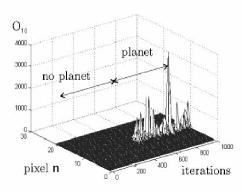
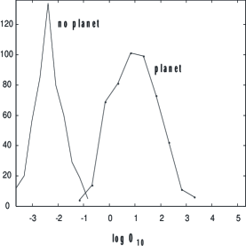
where Q=IpIb𝑄subscript𝐼𝑝subscript𝐼𝑏Q=\frac{I_{p}}{I_{b}} and Δ​Pj​(ΞΈ)Ξ”subscriptπ‘ƒπ‘—πœƒ\Delta P_{j}(\theta) is the area of the PSF covered by one of the five pixels (indexed by j𝑗j) when the planet appears at location ΞΈπœƒ\theta in pixel n𝑛n. Figure 1 depicts the results obtained for two simulated sets of images. For i∈[1,500]𝑖1500i\in[1,500], the data are simulated without any planet (Q=0𝑄0Q=0), while for i∈[501,1000]𝑖5011000i\in[501,1000], Q=1𝑄1Q=1, the planet is located in pixel nβˆ—=11superscript𝑛11n^{*}=11. For all simulations, the normalized integration time was set to Ο„=1𝜏1\tau=1, corresponding to a signal-to-noise ratio S/N𝑆𝑁S/N computed as in Eq.Β 1 of 3.523.523.52. While it is reasonable to expect some detections using the conventional approach with this S/N𝑆𝑁S/N ratio, using the usual criteria of S/N=5𝑆𝑁5S/N=5 described above, no planets would be detected. FigureΒ 2 depicts the histogram of log⁑O10nβˆ—superscriptsubscript𝑂10superscript𝑛\log O_{10}^{n^{*}} for the two simulated sets. For a threshold equal to one, the false alarm rate is 0.1%percent0.10.1\%, while the missed detection rate reaches 7.2%percent7.27.2\%. From the ROC curve (not plotted here for brevity), we determined that the test has maximal power if the threshold is set to 0.1580.1580.158 rather than 1. With this threshold, the false alarm rate is 4.0%percent4.04.0\% and the missed detection rate is 3.0%percent3.03.0\%. This demonstrates that under the same assumptions, the Bayesian technique is extremely effective at detection with quantifiable performance and at shorter integration times.
Refer to caption
Figure 1: Value of O10nsuperscriptsubscript𝑂10𝑛O_{10}^{n} as a function of n𝑛n for the two simulated sets, for Ο„=1𝜏1\tau=1.
Refer to caption
Figure 2: Histogram of log⁑O10nβˆ—superscriptsubscript𝑂10superscript𝑛\log O_{10}^{n^{*}} for the two simulated sets, Ο„=1𝜏1\tau=1

3.2 Assume Ipsubscript𝐼𝑝I_{p} is uncertain

The first complication to consider is a lack of knowledge of Ipsubscript𝐼𝑝I_{p}. In Kasdin etΒ al. (2003), we take the approach of estimating Ipsubscript𝐼𝑝I_{p} (whether a planet is there or not) and examining the quality of the estimate to make the decision. Here, we avoid photometry and still use a Bayesian hypothesis testing approach to make the decision in a shorter integration time.

If we assume under H1subscript𝐻1H_{1} that Ipsubscript𝐼𝑝I_{p} follows a gamma law, Γ​(Ξ±,Ξ²)Γ𝛼𝛽\Gamma(\alpha,\beta), then using Eqs.Β 3 and 4 we get

O10n=1Ξ”β€‹Ξ±β€‹βˆ‘p=0p=βˆ‘j=nβˆ’Kn+KzjΓ​(Ξ±+p)Γ​(Ξ±)​(Ξ²Ib)p​1(1+τ​β​Δ​P)Ξ±+pβ€‹βˆ«0Δ​αγp​(ΞΈ)​𝑑θsuperscriptsubscript𝑂10𝑛1Δ𝛼superscriptsubscript𝑝0𝑝superscriptsubscript𝑗𝑛𝐾𝑛𝐾subscript𝑧𝑗Γ𝛼𝑝Γ𝛼superscript𝛽subscript𝐼𝑏𝑝1superscript1πœπ›½Ξ”π‘ƒπ›Όπ‘superscriptsubscript0Δ𝛼subscriptπ›Ύπ‘πœƒdifferential-dπœƒO_{10}^{n}=\frac{1}{\Delta\alpha}\sum_{p=0}^{p=\sum_{j=n-K}^{n+K}z_{j}}\frac{\Gamma\left(\alpha+p\right)}{\Gamma\left(\alpha\right)}\left(\frac{\beta}{I_{b}}\right)^{p}\frac{1}{(1+\tau\beta\Delta P)^{\alpha+p}}\int_{0}^{\Delta\alpha}\gamma_{p}\left(\theta\right)d\theta (8)

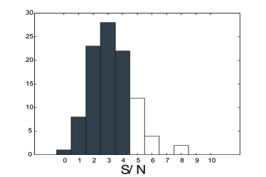
where the coefficients Ξ³p​(ΞΈ)subscriptπ›Ύπ‘πœƒ\gamma_{p}(\theta) are provided in the Appendix. The data have been simulated for Ο„=1𝜏1\tau=1, with Ξ±=4𝛼4\alpha=4 and Ξ²=Q​Ib/4𝛽𝑄subscript𝐼𝑏4\beta=QI_{b}/4. The histogram of the resulting estimated S/N𝑆𝑁S/N using Eq.Β 1 and the Ipsubscript𝐼𝑝I_{p} selected from the distribution from each run is depicted on FigureΒ 3. Following Eq.Β 1, if a conclusion is reached only for S/N>5𝑆𝑁5S/N>5, the missed detection rate reaches 72.7%. As described in Section 3.1, the mean value of Ipsubscript𝐼𝑝I_{p} was chosen to correspond to a S/N𝑆𝑁S/N of 3.52 for Ο„=1𝜏1\tau=1. When Ipsubscript𝐼𝑝I_{p} is sampled from the gamma distribution here (with the same mean value), roughly 24% of the time a planet occurs with a mean S/N>5𝑆𝑁5S/N>5 that would assure a detection by the conventional approach. For the same simulated data, our criterion provides a missed detection rate of only 1.0% with the odds ratio decision threshold set at one.
Refer to caption
Figure 3: Histograms of the estimated S/N𝑆𝑁S/N when the planet intensity Ipsubscript𝐼𝑝I_{p} follows a Gamma law. The blue boxes correspond to the case where S/N<5𝑆𝑁5S/N<5, i.e. that an existing planet has not been detected.
Refer to caption
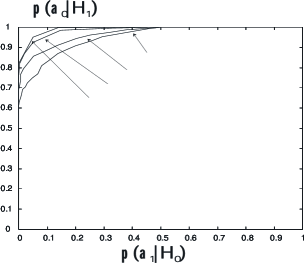
Figure 4: ROC curves as a function of the relative integration time Ο„πœ\tau: the power of the test increases with Ο„πœ\tau

The Receiver Operating Curves for this case is depicted in FigureΒ 4. It shows the trade-off between the false alarm and the missed detection rates for different values of the relative integration time Ο„πœ\tau. As expected, the greater Ο„πœ\tau, the more powerful the test. Nevertheless, note that a relatively high correct decision probability p​(a0|H0)+p​(a1|H1)𝑝conditionalsubscriptπ‘Ž0subscript𝐻0𝑝conditionalsubscriptπ‘Ž1subscript𝐻1p(a_{0}|H_{0})+p(a_{1}|H_{1}) (found via the Monte Carlo results with a decision threshold of one) can be achieved even for low integration times (see TableΒ 1). In practice on real data we may choose the lower optimal threshold deduced from the simulations, thus achieving slightly higher probabilities of success.

Ο„πœ\tau 0.10.10.1 0.20.20.2 0.50.50.5 111
p​(a0|H0)+p​(a1|H1)𝑝conditionalsubscriptπ‘Ž0subscript𝐻0𝑝conditionalsubscriptπ‘Ž1subscript𝐻1p(a_{0}|H_{0})+p(a_{1}|H_{1}) 0.7320.7320.732 0.8040.8040.804 0.8760.8760.876 0.9000.9000.900
Table 1: Evolution of the correct decision probability with Ο„πœ\tau

3.3 Assume Ibsubscript𝐼𝑏I_{b} is also unknown

The final, and most complicated, case is to assume that both Ipsubscript𝐼𝑝I_{p} and Ibsubscript𝐼𝑏I_{b} are unknown. Again, in our previous report and in Kasdin etΒ al. (2003), we resorted to two-parameter least-squares estimation (matched filtering) on the photometric data. By simultaneously estimating the irradiance of the planet and the background, a decision can be made on the planet, but the integration times become quite long. With the Bayesian approach, we found that we have a very high probability of success even at the same integration time as the previous case.

For the sake of brevity, we defer the derivation to the Appendix. If p​(Ib)=Γ​(a,b)𝑝subscriptπΌπ‘Ξ“π‘Žπ‘p(I_{b})=\Gamma(a,b), we use the marginalization law Eq.Β 4 to eliminate its dependence from the odds ratio and obtain:

O10n=1Δ​α​1(1+β​τ​Δ​P)Ξ±+pβ€‹βˆ‘p=0p=βˆ‘j=nβˆ’Kn+KzjΓ​(Ξ±+p)Γ​(Ξ±)​(Ξ²β€²bβ€²)p​Γ​(ΟƒKβˆ’p)Γ​(ΟƒK+a)β€‹βˆ«0Δ​αγp​(ΞΈ)​𝑑θsuperscriptsubscript𝑂10𝑛1Δ𝛼1superscript1π›½πœΞ”π‘ƒπ›Όπ‘superscriptsubscript𝑝0𝑝superscriptsubscript𝑗𝑛𝐾𝑛𝐾subscript𝑧𝑗Γ𝛼𝑝Γ𝛼superscriptsuperscript𝛽′superscript𝑏′𝑝ΓsubscriptπœŽπΎπ‘Ξ“subscriptπœŽπΎπ‘Žsuperscriptsubscript0Δ𝛼subscriptπ›Ύπ‘πœƒdifferential-dπœƒO_{10}^{n}=\frac{1}{\Delta\alpha}\frac{1}{\left(1+\beta\tau\Delta P\right)^{\alpha+p}}\sum_{p=0}^{p=\sum_{j=n-K}^{n+K}z_{j}}\frac{\Gamma\left(\alpha+p\right)}{\Gamma\left(\alpha\right)}\left(\frac{\beta^{\prime}}{b^{\prime}}\right)^{p}\frac{\Gamma\left(\sigma_{K}-p\right)}{\Gamma\left(\sigma_{K}+a\right)}\int_{0}^{\Delta\alpha}\gamma_{p}\left(\theta\right)d\theta

where

1bβ€²=1b+τ​Δ​S1superscript𝑏′1π‘πœΞ”π‘†\frac{1}{b^{\prime}}=\frac{1}{b}+\tau\Delta S

A similar Monte-Carlo study as before shows that we can reach a correct decision probability of 0.84 for the same integration time ( Ο„=1𝜏1\tau=1) with E​[Ip]E​[Ib]=1𝐸delimited-[]subscript𝐼𝑝𝐸delimited-[]subscript𝐼𝑏1\frac{E[I_{p}]}{E[I_{b}]}=1 and E​[Ip2]=E​[Ib]/2,E​[Ib2]=E​[Ib]/2formulae-sequence𝐸delimited-[]superscriptsubscript𝐼𝑝2𝐸delimited-[]subscript𝐼𝑏2𝐸delimited-[]superscriptsubscript𝐼𝑏2𝐸delimited-[]subscript𝐼𝑏2E[I_{p}^{2}]=E[I_{b}]/2,E[I_{b}^{2}]=E[I_{b}]/2.

4 Conclusion

Bayesian hypothesis testing is a promising approach to planet detection and to associate a quantitative confidence level with the detection system, with a relative integration time smaller than t1subscript𝑑1t_{1} and without performing photometry. Moreover this approach allows us to take into account the uncertainty associated with the nuisance parameters such as the intensity of the background via the marginalization law. Nevertheless, choosing a prior may strongly influence the quality of the result. Further work aims to develop this same approach with other priors and to study its robustness.

No speckle has been considered yet. Current work aims at defining a three-hypothesis test to detect if the pixel under study contains a planet, speckle, or just noise. A trio of three bandpass filters, while allowing us to consider quasi-monochromatic signals (and directly applying this technique), would also permit us to define speckle as a space-variant component. Note that adding other features in addition to just the PSF shape in a Bayesian or optimal classifier could also improve the results.

References

  • Brown etΒ al. (2002) R.Β A. Brown, C.Β J. Burrows, S.Β Casertano, M.Β Clampin, D.Β Eggets, E.B. Ford, K.W. Jucks, N.Β J. Kasdin, S.Β Kilston, M.Β J. Kuchner, S.Β Seager, A.Β Sozzetti, D.Β N. Spergel, W.Β A. Traub, J.Β T. Trauger, and E.Β L. Turner. The 4-meter space telescope for investigating extrasolar earth-like planets in starlight: TPF is HST2. In Proceedings of SPIE: Astronomical Telescopes and Instrumentation, numberΒ 14 in 4860, 2002.
  • Kasdin etΒ al. (2003) N.Β J. Kasdin, R.Β J. Vanderbei, D.Β N. Spergel, and M.Β G. Littman. Extrasolar planet finding via optimal apodized-pupil and shaped-pupil coronagraphs. The Astrophysical Journal, 582:1147–1161, January 2003.
  • Vanderbei etΒ al. (2003a) R.J. Vanderbei, D.N. Spergel, and N.J. Kasdin. Spiderweb Masks for High Contrast Imaging. Astrophysical Journal, 590:593–603, June 10 2003a.
  • Vanderbei etΒ al. (2003b) R.J. Vanderbei, D.N. Spergel, and N.J. Kasdin. Circularly Symmetric Apodization via Starshaped Masks. Astrophysical Journal, 599(1):686–694, December 10 2003b.
  • Brown and Burrows (1990) R.Β A. Brown and C.Β J. Burrows. On the feasibility of detecting extrasolar planets by reflected starlight using the hubble space telescope. Icarus, 87:484–497, 1990.
  • Berger (1985) J.Β Berger. Satistical decision theory and Bayesian analysis. Springer-Verlag, 1985.
  • Loredo (1992) T.Β Loredo. The promise of bayesian inference for astrophysics. In Statistical Challenges in Modern Astronomy, pages 275–297. Springer-Verlag, 1992.
  • Gregory and Loredo (1992) P.Β Gregory and T.Β Loredo. A new method for the detection of a periodic signal of unknown shape and period. The Astropohysical Journal, 298:146–168, 1992.
  • Defay etΒ al. (2001) C.Β Defay, M.Β Deleuil, and P.Β Barge. A bayesian method for the detection of planetary transits. Astronomy and Astrophysics, 365(2):330–340, 2001.
  • Aigrain and Favata (2002) S.Β Aigrain and F.Β Favata. Bayesian detection of planetary transits: a modified version of the gregory-loredo method for bayesian periodic signal detection. Astronomy and Astrophysics, 395:625–636, 2002.

Appendix A Appendix

A.1 PSF Truncation

Let ΔΔ\Delta be the FWHM of the PSF. The maximum number of pixels that can be covered by the PSF is an even number denoted by 2​K+12𝐾12K+1 where

K=c​e​i​l​(ΔΔ​α).𝐾𝑐𝑒𝑖𝑙ΔΔ𝛼K=ceil\left(\frac{\Delta}{\Delta\alpha}\right).

As

p​(zk|M1n)=p​(zk|M0),kβˆ‰[nβˆ’K,n+K]formulae-sequence𝑝conditionalsubscriptπ‘§π‘˜superscriptsubscript𝑀1𝑛𝑝conditionalsubscriptπ‘§π‘˜subscript𝑀0π‘˜π‘›πΎπ‘›πΎp\left(z_{k}|M_{1}^{n}\right)=p\left(z_{k}|M_{0}\right),k\notin\left[n-K,n+K\right]

Then

O10n=∏k=1Mp​(zk|M1n)∏k=1Mp​(zk|M0n)=∏k=nβˆ’Kn+Kp​(zk|M1n)∏k=nβˆ’Kn+Kp​(zk|M0n)β‰œL1​(Ip,Ib,ΞΈ)L0​(Ib)superscriptsubscript𝑂10𝑛superscriptsubscriptproductπ‘˜1𝑀𝑝conditionalsubscriptπ‘§π‘˜superscriptsubscript𝑀1𝑛superscriptsubscriptproductπ‘˜1𝑀𝑝conditionalsubscriptπ‘§π‘˜superscriptsubscript𝑀0𝑛superscriptsubscriptproductπ‘˜π‘›πΎπ‘›πΎπ‘conditionalsubscriptπ‘§π‘˜superscriptsubscript𝑀1𝑛superscriptsubscriptproductπ‘˜π‘›πΎπ‘›πΎπ‘conditionalsubscriptπ‘§π‘˜superscriptsubscript𝑀0π‘›β‰œsubscript𝐿1subscript𝐼𝑝subscriptπΌπ‘πœƒsubscript𝐿0subscript𝐼𝑏O_{10}^{n}=\frac{\prod\limits_{k=1}^{M}p\left(z_{k}|M_{1}^{n}\right)}{\prod\limits_{k=1}^{M}p\left(z_{k}|M_{0}^{n}\right)}=\frac{\prod\limits_{k=n-K}^{n+K}p\left(z_{k}|M_{1}^{n}\right)}{\prod\limits_{k=n-K}^{n+K}p\left(z_{k}|M_{0}^{n}\right)}\triangleq\frac{L_{1}\left(I_{p},I_{b},\theta\right)}{L_{0}\left(I_{b}\right)}

Example. If K=1,𝐾1K=1, 3 pixels only can be involved,

O10n=p​(znβˆ’1|M1n)​p​(zn|M1n)​p​(zn+1|M1n)p​(znβˆ’1|M0n)​p​(zn|M0n)​p​(zn+1|M0n)superscriptsubscript𝑂10𝑛𝑝conditionalsubscript𝑧𝑛1superscriptsubscript𝑀1𝑛𝑝conditionalsubscript𝑧𝑛superscriptsubscript𝑀1𝑛𝑝conditionalsubscript𝑧𝑛1superscriptsubscript𝑀1𝑛𝑝conditionalsubscript𝑧𝑛1superscriptsubscript𝑀0𝑛𝑝conditionalsubscript𝑧𝑛superscriptsubscript𝑀0𝑛𝑝conditionalsubscript𝑧𝑛1superscriptsubscript𝑀0𝑛O_{10}^{n}=\frac{p\left(z_{n-1}|M_{1}^{n}\right)p\left(z_{n}|M_{1}^{n}\right)p\left(z_{n+1}|M_{1}^{n}\right)}{p\left(z_{n-1}|M_{0}^{n}\right)p\left(z_{n}|M_{0}^{n}\right)p\left(z_{n+1}|M_{0}^{n}\right)}

In the following, we will use the following notation

ΟƒKβ‰œβˆ‘k=nβˆ’Kk=n+Kzk;Ο€kβ‰œβˆk=nβˆ’Kn+Kzk!formulae-sequenceβ‰œsubscript𝜎𝐾superscriptsubscriptπ‘˜π‘›πΎπ‘˜π‘›πΎsubscriptπ‘§π‘˜β‰œsubscriptπœ‹π‘˜superscriptsubscriptproductπ‘˜π‘›πΎπ‘›πΎsubscriptπ‘§π‘˜\sigma_{K}\triangleq\sum\limits_{k=n-K}^{k=n+K}z_{k};\pi_{k}\triangleq\prod\limits_{k=n-K}^{n+K}z_{k}!

A.2 Ip is assumed to be known

Obviously, as Ibsubscript𝐼𝑏I_{b} is assumed to be known

p​(Z|M0n)=βˆ«β„p​(Z|M0n,Ib)​p​(Ib)​𝑑Ib=p​(Z|M0n,Ib).𝑝conditional𝑍superscriptsubscript𝑀0𝑛subscriptℝ𝑝conditional𝑍superscriptsubscript𝑀0𝑛subscript𝐼𝑏𝑝subscript𝐼𝑏differential-dsubscript𝐼𝑏𝑝conditional𝑍superscriptsubscript𝑀0𝑛subscript𝐼𝑏p\left(Z|M_{0}^{n}\right)=\int_{\mathbb{R}}p\left(Z|M_{0}^{n},I_{b}\right)p\left(I_{b}\right)dI_{b}=p\left(Z|M_{0}^{n},I_{b}\right).

For the constant-rate model M0nsuperscriptsubscript𝑀0𝑛M_{0}^{n}

L0​(Ib)=∏k=nβˆ’Kn+Kp​(zk|M0n,Ib)=∏k=nβˆ’Kn+K1zk!​λkzk​exp⁑(βˆ’Ξ»k)subscript𝐿0subscript𝐼𝑏superscriptsubscriptproductπ‘˜π‘›πΎπ‘›πΎπ‘conditionalsubscriptπ‘§π‘˜superscriptsubscript𝑀0𝑛subscript𝐼𝑏superscriptsubscriptproductπ‘˜π‘›πΎπ‘›πΎ1subscriptπ‘§π‘˜superscriptsubscriptπœ†π‘˜subscriptπ‘§π‘˜subscriptπœ†π‘˜\displaystyle L_{0}\left(I_{b}\right)=\prod\limits_{k=n-K}^{n+K}p\left(z_{k}|M_{0}^{n},I_{b}\right)=\prod\limits_{k=n-K}^{n+K}\frac{1}{z_{k}!}\lambda_{k}^{z_{k}}\exp\left(-\lambda_{k}\right)
=\displaystyle= ∏k=nβˆ’Kn+K1zk!​(Ib​Δ​α​τ)zk​exp⁑(βˆ’Ib​Δ​α​τ)=1Ο€K​(Ib​τ​Δ​α)ΟƒK​exp⁑(βˆ’Ib​τ​Δ​S),superscriptsubscriptproductπ‘˜π‘›πΎπ‘›πΎ1subscriptπ‘§π‘˜superscriptsubscriptπΌπ‘Ξ”π›Όπœsubscriptπ‘§π‘˜subscriptπΌπ‘Ξ”π›Όπœ1subscriptπœ‹πΎsuperscriptsubscriptπΌπ‘πœΞ”π›Όsubscript𝜎𝐾subscriptπΌπ‘πœΞ”π‘†\displaystyle\prod\limits_{k=n-K}^{n+K}\frac{1}{z_{k}!}\left(I_{b}\Delta\alpha\tau\right)^{z_{k}}\exp\left(-I_{b}\Delta\alpha\tau\right)=\frac{1}{\pi_{K}}\left(I_{b}\tau\Delta\alpha\right)^{\sigma_{K}}\exp\left(-I_{b}\tau\Delta S\right),

where Δ​S=(2​K+1)​Δ​αΔ𝑆2𝐾1Δ𝛼\Delta S=\left(2K+1\right)\Delta\alpha is the area of integration around the n′​t​hsuperscriptπ‘›β€²π‘‘β„Žn^{\prime}th pixel.

Assuming that ΞΈπœƒ\theta is uniform on [ΞΆn,ΞΆn+1]subscriptπœπ‘›subscriptπœπ‘›1\left[\zeta_{n},\zeta_{n+1}\right], the likelihood of the alternative model M1nsuperscriptsubscript𝑀1𝑛M_{1}^{n} is

L1​(Ip,Ib)subscript𝐿1subscript𝐼𝑝subscript𝐼𝑏\displaystyle L_{1}\left(I_{p},I_{b}\right) =\displaystyle= ∫΢nΞΆn+1p​(Z|M1n,Ib,Ip,ΞΈ)​p​(ΞΈ)​𝑑θsuperscriptsubscriptsubscriptπœπ‘›subscriptπœπ‘›1𝑝conditional𝑍superscriptsubscript𝑀1𝑛subscript𝐼𝑏subscriptπΌπ‘πœƒπ‘πœƒdifferential-dπœƒ\displaystyle\int_{\zeta_{n}}^{\zeta_{n+1}}p\left(Z|M_{1}^{n},I_{b},I_{p},\theta\right)p\left(\theta\right)d\theta
=\displaystyle= 1Ξ”β€‹Ξ±β€‹βˆ«ΞΆnΞΆn+1π‘‘ΞΈβ€‹βˆk=nβˆ’Kn+Kp​(zk|M1n,Ib,Ip,ΞΈ)1Δ𝛼superscriptsubscriptsubscriptπœπ‘›subscriptπœπ‘›1differential-dπœƒsuperscriptsubscriptproductπ‘˜π‘›πΎπ‘›πΎπ‘conditionalsubscriptπ‘§π‘˜superscriptsubscript𝑀1𝑛subscript𝐼𝑏subscriptπΌπ‘πœƒ\displaystyle\frac{1}{\Delta\alpha}\int_{\zeta_{n}}^{\zeta_{n+1}}d\theta\prod\limits_{k=n-K}^{n+K}p\left(z_{k}|M_{1}^{n},I_{b},I_{p},\theta\right)
=\displaystyle= 1Ξ”β€‹Ξ±β€‹βˆ«ΞΆnΞΆn+1𝑑θ​1Ο€Kβ€‹βˆk=nβˆ’Kn+K(Ib​Δ​α​τ+Ip​Δ​Pk​(ΞΈ))zk​exp⁑(βˆ’Ο„β€‹(Ib​Δ​α+Ip​Δ​Pk​(ΞΈ)))1Δ𝛼superscriptsubscriptsubscriptπœπ‘›subscriptπœπ‘›1differential-dπœƒ1subscriptπœ‹πΎsuperscriptsubscriptproductπ‘˜π‘›πΎπ‘›πΎsuperscriptsubscriptπΌπ‘Ξ”π›Όπœsubscript𝐼𝑝Δsubscriptπ‘ƒπ‘˜πœƒsubscriptπ‘§π‘˜πœsubscript𝐼𝑏Δ𝛼subscript𝐼𝑝Δsubscriptπ‘ƒπ‘˜πœƒ\displaystyle\frac{1}{\Delta\alpha}\int_{\zeta_{n}}^{\zeta_{n+1}}d\theta\frac{1}{\pi_{K}}\prod\limits_{k=n-K}^{n+K}\left(I_{b}\Delta\alpha\tau+I_{p}\Delta P_{k}\left(\theta\right)\right)^{z_{k}}\exp\left(-\tau\left(I_{b}\Delta\alpha+I_{p}\Delta P_{k}\left(\theta\right)\right)\right)

Compute

A1​(ΞΈ)subscript𝐴1πœƒ\displaystyle A_{1}\left(\theta\right) =\displaystyle= ∏k=nβˆ’Kn+K(Ib​Δ​α​τ+τ​Ip​Δ​Pk​(ΞΈ))zk​exp⁑(βˆ’Ο„β€‹(Ib​Δ​α+Ip​Δ​Pk​(ΞΈ)))superscriptsubscriptproductπ‘˜π‘›πΎπ‘›πΎsuperscriptsubscriptπΌπ‘Ξ”π›Όπœπœsubscript𝐼𝑝Δsubscriptπ‘ƒπ‘˜πœƒsubscriptπ‘§π‘˜πœsubscript𝐼𝑏Δ𝛼subscript𝐼𝑝Δsubscriptπ‘ƒπ‘˜πœƒ\displaystyle\prod\limits_{k=n-K}^{n+K}\left(I_{b}\Delta\alpha\tau+\tau I_{p}\Delta P_{k}\left(\theta\right)\right)^{z_{k}}\exp\left(-\tau\left(I_{b}\Delta\alpha+I_{p}\Delta P_{k}\left(\theta\right)\right)\right)
=\displaystyle= (Ib​τ​Δ​α)ΟƒK​exp⁑(βˆ’Ib​τ​Δ​S)β€‹βˆk=nβˆ’Kn+K(1+Ip​Δ​Pk​(ΞΈ)Ib​τ​Δ​α)zk​exp⁑(βˆ’Ο„β€‹βˆ‘k=nβˆ’Kk=n+KIp​Δ​Pk​(ΞΈ))superscriptsubscriptπΌπ‘πœΞ”π›Όsubscript𝜎𝐾subscriptπΌπ‘πœΞ”π‘†superscriptsubscriptproductπ‘˜π‘›πΎπ‘›πΎsuperscript1subscript𝐼𝑝Δsubscriptπ‘ƒπ‘˜πœƒsubscriptπΌπ‘πœΞ”π›Όsubscriptπ‘§π‘˜πœsuperscriptsubscriptπ‘˜π‘›πΎπ‘˜π‘›πΎsubscript𝐼𝑝Δsubscriptπ‘ƒπ‘˜πœƒ\displaystyle\left(I_{b}\tau\Delta\alpha\right)^{\sigma_{K}}\exp\left(-I_{b}\tau\Delta S\right)\prod\limits_{k=n-K}^{n+K}\left(1+\frac{I_{p}\Delta P_{k}\left(\theta\right)}{I_{b}\tau\Delta\alpha}\right)^{z_{k}}\exp\left(-\tau\sum\limits_{k=n-K}^{k=n+K}I_{p}\Delta P_{k}\left(\theta\right)\right)
=\displaystyle= (Ib​τ​Δ​α)ΟƒK​exp⁑(βˆ’Ο„β€‹(Ib​Δ​S+Ip​Δ​P))β€‹βˆk=nβˆ’Kn+K(1+Q​Δ​Pk​(ΞΈ)Δ​α)zksuperscriptsubscriptπΌπ‘πœΞ”π›Όsubscript𝜎𝐾𝜏subscript𝐼𝑏Δ𝑆subscript𝐼𝑝Δ𝑃superscriptsubscriptproductπ‘˜π‘›πΎπ‘›πΎsuperscript1𝑄Δsubscriptπ‘ƒπ‘˜πœƒΞ”π›Όsubscriptπ‘§π‘˜\displaystyle\left(I_{b}\tau\Delta\alpha\right)^{\sigma_{K}}\exp\left(-\tau\left(I_{b}\Delta S+I_{p}\Delta P\right)\right)\prod\limits_{k=n-K}^{n+K}\left(1+Q\frac{\Delta P_{k}\left(\theta\right)}{\Delta\alpha}\right)^{z_{k}}

by noting that βˆ‘k=nβˆ’Kk=n+KΔ​Pk​(ΞΈ)=Δ​Psuperscriptsubscriptπ‘˜π‘›πΎπ‘˜π‘›πΎΞ”subscriptπ‘ƒπ‘˜πœƒΞ”π‘ƒ\sum\limits_{k=n-K}^{k=n+K}\Delta P_{k}\left(\theta\right)=\Delta P and by noting Q=IpIb𝑄subscript𝐼𝑝subscript𝐼𝑏Q=\frac{I_{p}}{I_{b}}. We then have

L1​(Ip,Ib)=(Ib​τ​Δ​α)ΟƒKΔ​α​πK​exp⁑(βˆ’Ο„β€‹(Ib​Δ​S+Ip​Δ​P))β€‹βˆ«ΞΆnΞΆn+1π‘‘ΞΈβ€‹βˆk=nβˆ’Kn+K(1+Q​Δ​Pk​(ΞΈ)Δ​α)zksubscript𝐿1subscript𝐼𝑝subscript𝐼𝑏superscriptsubscriptπΌπ‘πœΞ”π›ΌsubscriptπœŽπΎΞ”π›Όsubscriptπœ‹πΎπœsubscript𝐼𝑏Δ𝑆subscript𝐼𝑝Δ𝑃superscriptsubscriptsubscriptπœπ‘›subscriptπœπ‘›1differential-dπœƒsuperscriptsubscriptproductπ‘˜π‘›πΎπ‘›πΎsuperscript1𝑄Δsubscriptπ‘ƒπ‘˜πœƒΞ”π›Όsubscriptπ‘§π‘˜L_{1}\left(I_{p},I_{b}\right)=\frac{\left(I_{b}\tau\Delta\alpha\right)^{\sigma_{K}}}{\Delta\alpha\pi_{K}}\exp\left(-\tau\left(I_{b}\Delta S+I_{p}\Delta P\right)\right)\int_{\zeta_{n}}^{\zeta_{n+1}}d\theta\prod\limits_{k=n-K}^{n+K}\left(1+Q\frac{\Delta P_{k}\left(\theta\right)}{\Delta\alpha}\right)^{z_{k}}
O10n​(Ip,Ib)superscriptsubscript𝑂10𝑛subscript𝐼𝑝subscript𝐼𝑏\displaystyle O_{10}^{n}\left(I_{p},I_{b}\right) =\displaystyle= L1​(Ip,Ib)L0​(Ib)subscript𝐿1subscript𝐼𝑝subscript𝐼𝑏subscript𝐿0subscript𝐼𝑏\displaystyle\frac{L_{1}\left(I_{p},I_{b}\right)}{L_{0}\left(I_{b}\right)}
=\displaystyle= 1Δ​α​exp⁑(βˆ’Ο„β€‹Ip​Δ​P)β€‹βˆ«ΞΆnΞΆn+1π‘‘ΞΈβ€‹βˆk=nβˆ’Kn+K(1+Q​Δ​Pk​(ΞΈ)Δ​α)zk1Ξ”π›Όπœsubscript𝐼𝑝Δ𝑃superscriptsubscriptsubscriptπœπ‘›subscriptπœπ‘›1differential-dπœƒsuperscriptsubscriptproductπ‘˜π‘›πΎπ‘›πΎsuperscript1𝑄Δsubscriptπ‘ƒπ‘˜πœƒΞ”π›Όsubscriptπ‘§π‘˜\displaystyle\frac{1}{\Delta\alpha}\exp\left(-\tau I_{p}\Delta P\right)\int_{\zeta_{n}}^{\zeta_{n+1}}d\theta\prod\limits_{k=n-K}^{n+K}\left(1+Q\frac{\Delta P_{k}\left(\theta\right)}{\Delta\alpha}\right)^{z_{k}}

A.3 Assume Ipsubscript𝐼𝑝I_{p} is uncertain

As Ibsubscript𝐼𝑏I_{b} is still assumed to be known, L0subscript𝐿0L_{0} is unchanged. Using the marginalization law, we have

O10n​(Ib)superscriptsubscript𝑂10𝑛subscript𝐼𝑏\displaystyle O_{10}^{n}\left(I_{b}\right) =\displaystyle= ∫0∞p​(Ip)​L1​(Ip)​𝑑IpL0​(Ib)superscriptsubscript0𝑝subscript𝐼𝑝subscript𝐿1subscript𝐼𝑝differential-dsubscript𝐼𝑝subscript𝐿0subscript𝐼𝑏\displaystyle\frac{\int_{0}^{\infty}p\left(I_{p}\right)L_{1}\left(I_{p}\right)dI_{p}}{L_{0}\left(I_{b}\right)}
=\displaystyle= 1Ξ”β€‹Ξ±β€‹βˆ«π‘‘Ip​p​(Ip)​exp⁑(βˆ’Ο„β€‹Ip​Δ​P)β€‹βˆ«ΞΆnΞΆn+1π‘‘ΞΈβ€‹βˆk=nβˆ’Kn+K(1+IpIb​Δ​Pk​(ΞΈ)Δ​α)zk1Δ𝛼differential-dsubscript𝐼𝑝𝑝subscriptπΌπ‘πœsubscript𝐼𝑝Δ𝑃superscriptsubscriptsubscriptπœπ‘›subscriptπœπ‘›1differential-dπœƒsuperscriptsubscriptproductπ‘˜π‘›πΎπ‘›πΎsuperscript1subscript𝐼𝑝subscript𝐼𝑏Δsubscriptπ‘ƒπ‘˜πœƒΞ”π›Όsubscriptπ‘§π‘˜\displaystyle\frac{1}{\Delta\alpha}\int dI_{p}p\left(I_{p}\right)\exp\left(-\tau I_{p}\Delta P\right)\int_{\zeta_{n}}^{\zeta_{n+1}}d\theta\prod\limits_{k=n-K}^{n+K}\left(1+\frac{I_{p}}{I_{b}}\frac{\Delta P_{k}\left(\theta\right)}{\Delta\alpha}\right)^{z_{k}}
=\displaystyle= 1Δ​α​Γ​(Ξ±)β€‹Ξ²Ξ±β€‹βˆ«ΞΆnΞΆn+1π‘‘ΞΈβ€‹βˆ«0βˆžπ‘‘Ip​IpΞ±βˆ’1​exp⁑(βˆ’IpΞ²β€²)β€‹βˆk=nβˆ’Kn+K(1+Ip​Δ​Pk​(ΞΈ)Ib​Δ​α)zk,1Δ𝛼Γ𝛼superscript𝛽𝛼superscriptsubscriptsubscriptπœπ‘›subscriptπœπ‘›1differential-dπœƒsuperscriptsubscript0differential-dsubscript𝐼𝑝superscriptsubscript𝐼𝑝𝛼1subscript𝐼𝑝superscript𝛽′superscriptsubscriptproductπ‘˜π‘›πΎπ‘›πΎsuperscript1subscript𝐼𝑝Δsubscriptπ‘ƒπ‘˜πœƒsubscript𝐼𝑏Δ𝛼subscriptπ‘§π‘˜\displaystyle\frac{1}{\Delta\alpha\Gamma\left(\alpha\right)\beta^{\alpha}}\int_{\zeta_{n}}^{\zeta_{n+1}}d\theta\int_{0}^{\infty}dI_{p}I_{p}^{\alpha-1}\exp\left(-\frac{I_{p}}{\beta^{\prime}}\right)\prod\limits_{k=n-K}^{n+K}\left(1+I_{p}\frac{\Delta P_{k}\left(\theta\right)}{I_{b}\Delta\alpha}\right)^{z_{k}},

by posing

1Ξ²β€²=1Ξ²+τ​Δ​P1superscript𝛽′1π›½πœΞ”π‘ƒ\frac{1}{\beta^{\prime}}=\frac{1}{\beta}+\tau\Delta P

For the sake of simplicity, we only present here the case for K=2𝐾2K=2 (case described in the main document).

Using the binomial law

(1+α​x)Ξ²=βˆ‘n=0Ξ²(Ξ²n)​αn​xnsuperscript1𝛼π‘₯𝛽superscriptsubscript𝑛0𝛽binomial𝛽𝑛superscript𝛼𝑛superscriptπ‘₯𝑛\left(1+\alpha x\right)^{\beta}=\sum_{n=0}^{\beta}\binom{\beta}{n}\alpha^{n}x^{n}

2​K+12𝐾12K+1 times we have that

∏k=nβˆ’Kn+K(1+Ip​Δ​Pk​(ΞΈ)Ib​Δ​α)zk=βˆ‘p=0ΟƒKΞ³p​(ΞΈ)​(IpIb)psuperscriptsubscriptproductπ‘˜π‘›πΎπ‘›πΎsuperscript1subscript𝐼𝑝Δsubscriptπ‘ƒπ‘˜πœƒsubscript𝐼𝑏Δ𝛼subscriptπ‘§π‘˜superscriptsubscript𝑝0subscript𝜎𝐾subscriptπ›Ύπ‘πœƒsuperscriptsubscript𝐼𝑝subscript𝐼𝑏𝑝\prod\limits_{k=n-K}^{n+K}\left(1+I_{p}\frac{\Delta P_{k}\left(\theta\right)}{I_{b}\Delta\alpha}\right)^{z_{k}}=\sum_{p=0}^{\sigma_{K}}\gamma_{p}\left(\theta\right)\left(\frac{I_{p}}{I_{b}}\right)^{p}

where

Ξ³p​(ΞΈ)subscriptπ›Ύπ‘πœƒ\displaystyle\gamma_{p}\left(\theta\right) =\displaystyle= βˆ‘r=max⁑(0,pβˆ’zn+1)min⁑(βˆ‘nβˆ’Knzj,p)Ξ²r​(ΞΈ)​(zn+1pβˆ’r)​(Δ​Pn+1​(ΞΈ)Δ​α)pβˆ’r;superscriptsubscriptπ‘Ÿ0𝑝subscript𝑧𝑛1superscriptsubscript𝑛𝐾𝑛subscript𝑧𝑗𝑝subscriptπ›½π‘Ÿπœƒbinomialsubscript𝑧𝑛1π‘π‘ŸsuperscriptΞ”subscript𝑃𝑛1πœƒΞ”π›Όπ‘π‘Ÿ\displaystyle\sum_{r=\max\left(0,p-z_{n+1}\right)}^{\min\left(\sum_{n-K}^{n}z_{j},p\right)}\beta_{r}\left(\theta\right)\binom{z_{n+1}}{p-r}\left(\frac{\Delta P_{n+1}\left(\theta\right)}{\Delta\alpha}\right)^{p-r};
Ξ²r​(ΞΈ)subscriptπ›½π‘Ÿπœƒ\displaystyle\beta_{r}\left(\theta\right) =\displaystyle= βˆ‘l=max⁑(0,rβˆ’znβˆ’zn+1)min⁑(znβˆ’K+znβˆ’K+1,r)Ξ±l​(ΞΈ,n,n+1)​αpβˆ’l​(ΞΈ,n+2,n+3)superscriptsubscript𝑙0π‘Ÿsubscript𝑧𝑛subscript𝑧𝑛1subscript𝑧𝑛𝐾subscript𝑧𝑛𝐾1π‘Ÿsubscriptπ›Όπ‘™πœƒπ‘›π‘›1subscriptπ›Όπ‘π‘™πœƒπ‘›2𝑛3\displaystyle\sum_{l=\max\left(0,r-z_{n}-z_{n+1}\right)}^{\min\left(z_{n-K}+z_{n-K+1},r\right)}\alpha_{l}\left(\theta,n,n+1\right)\alpha_{p-l}\left(\theta,n+2,n+3\right)
Ξ±l​(ΞΈ,i,j)subscriptπ›Όπ‘™πœƒπ‘–π‘—\displaystyle\alpha_{l}\left(\theta,i,j\right) =\displaystyle= βˆ‘m=max⁑(0,lβˆ’zj)min⁑(zi,l)(zim)​(zjlβˆ’m)​(Δ​Pi​(ΞΈ)Δ​α)m​(Δ​Pj​(ΞΈ)Δ​α)lβˆ’msuperscriptsubscriptπ‘š0𝑙subscript𝑧𝑗subscript𝑧𝑖𝑙binomialsubscriptπ‘§π‘–π‘šbinomialsubscriptπ‘§π‘—π‘™π‘šsuperscriptΞ”subscriptπ‘ƒπ‘–πœƒΞ”π›Όπ‘šsuperscriptΞ”subscriptπ‘ƒπ‘—πœƒΞ”π›Όπ‘™π‘š\displaystyle\sum_{m=\max\left(0,l-z_{j}\right)}^{\min\left(z_{i},l\right)}\binom{z_{i}}{m}\binom{z_{j}}{l-m}\left(\frac{\Delta P_{i}\left(\theta\right)}{\Delta\alpha}\right)^{m}\left(\frac{\Delta P_{j}\left(\theta\right)}{\Delta\alpha}\right)^{l-m}

so that

O10n​(Ib)superscriptsubscript𝑂10𝑛subscript𝐼𝑏\displaystyle O_{10}^{n}\left(I_{b}\right) =\displaystyle= 1Δ​α​Γ​(Ξ±)β€‹Ξ²Ξ±β€‹βˆ«ΞΆnΞΆn+1π‘‘ΞΈβ€‹βˆ«0βˆžπ‘‘Ip​IpΞ±βˆ’1​exp⁑(βˆ’IpΞ²β€²)β€‹βˆ‘pΞ³p​(ΞΈ)​(IpIb)p1Δ𝛼Γ𝛼superscript𝛽𝛼superscriptsubscriptsubscriptπœπ‘›subscriptπœπ‘›1differential-dπœƒsuperscriptsubscript0differential-dsubscript𝐼𝑝superscriptsubscript𝐼𝑝𝛼1subscript𝐼𝑝superscript𝛽′subscript𝑝subscriptπ›Ύπ‘πœƒsuperscriptsubscript𝐼𝑝subscript𝐼𝑏𝑝\displaystyle\frac{1}{\Delta\alpha\Gamma\left(\alpha\right)\beta^{\alpha}}\int_{\zeta_{n}}^{\zeta_{n+1}}d\theta\int_{0}^{\infty}dI_{p}I_{p}^{\alpha-1}\exp\left(-\frac{I_{p}}{\beta^{\prime}}\right)\sum_{p}\gamma_{p}\left(\theta\right)\left(\frac{I_{p}}{I_{b}}\right)^{p}
=\displaystyle= 1Δ​α​Γ​(Ξ±)β€‹Ξ²Ξ±β€‹βˆ‘p1Ibpβ€‹βˆ«ΞΆnΞΆn+1Ξ³p​(ΞΈ)β€‹π‘‘ΞΈβ€‹βˆ«0βˆžπ‘‘Ip​Ipp+Ξ±βˆ’1​exp⁑(βˆ’IpΞ²β€²)1Δ𝛼Γ𝛼superscript𝛽𝛼subscript𝑝1superscriptsubscript𝐼𝑏𝑝superscriptsubscriptsubscriptπœπ‘›subscriptπœπ‘›1subscriptπ›Ύπ‘πœƒdifferential-dπœƒsuperscriptsubscript0differential-dsubscript𝐼𝑝superscriptsubscript𝐼𝑝𝑝𝛼1subscript𝐼𝑝superscript𝛽′\displaystyle\frac{1}{\Delta\alpha\Gamma\left(\alpha\right)\beta^{\alpha}}\sum_{p}\frac{1}{I_{b}^{p}}\int_{\zeta_{n}}^{\zeta_{n+1}}\gamma_{p}\left(\theta\right)d\theta\int_{0}^{\infty}dI_{p}I_{p}^{p+\alpha-1}\exp\left(-\frac{I_{p}}{\beta^{\prime}}\right)
=\displaystyle= 1Δ​α​Γ​(Ξ±)β€‹Ξ²Ξ±β€‹βˆ‘p1Ibpβ€‹βˆ«ΞΆnΞΆn+1Ξ³p​(ΞΈ)​𝑑θ​Γ​(Ξ±+p)​β′α+p\displaystyle\frac{1}{\Delta\alpha\Gamma\left(\alpha\right)\beta^{\alpha}}\sum_{p}\frac{1}{I_{b}^{p}}\int_{\zeta_{n}}^{\zeta_{n+1}}\gamma_{p}\left(\theta\right)d\theta\Gamma\left(\alpha+p\right)\beta^{\prime^{\alpha+p}}

so

O10n​(Ib)=1Ξ”β€‹Ξ±β€‹βˆ‘pΓ​(Ξ±+p)Γ​(Ξ±)​(11+τ​Δ​P​β)Ξ±+p​(Ξ²Ib)pβ€‹βˆ«0Δ​αγp​(ΞΈ)​𝑑θ.superscriptsubscript𝑂10𝑛subscript𝐼𝑏1Δ𝛼subscript𝑝Γ𝛼𝑝Γ𝛼superscript11πœΞ”π‘ƒπ›½π›Όπ‘superscript𝛽subscript𝐼𝑏𝑝superscriptsubscript0Δ𝛼subscriptπ›Ύπ‘πœƒdifferential-dπœƒO_{10}^{n}\left(I_{b}\right)=\frac{1}{\Delta\alpha}\sum_{p}\frac{\Gamma\left(\alpha+p\right)}{\Gamma\left(\alpha\right)}\left(\frac{1}{1+\tau\Delta P\beta}\right)^{\alpha+p}\left(\frac{\beta}{I_{b}}\right)^{p}\int_{0}^{\Delta\alpha}\gamma_{p}\left(\theta\right)d\theta.

Remark. Note that the computation of ∫0Δ​αγp​(ΞΈ)​𝑑θsuperscriptsubscript0Δ𝛼subscriptπ›Ύπ‘πœƒdifferential-dπœƒ\int_{0}^{\Delta\alpha}\gamma_{p}\left(\theta\right)d\theta, that may look very time-consuming, can be done before any data are collected. To be computed, only the sums (depending on zisubscript𝑧𝑖z_{i}) have to be computed online.

A.4 When Ib is uncertain

We now have to apply the marginalization law for both sides.

L0subscript𝐿0\displaystyle L_{0} =\displaystyle= ∫0∞p​(Ib)​L0​(Ib)​𝑑Ibsuperscriptsubscript0𝑝subscript𝐼𝑏subscript𝐿0subscript𝐼𝑏differential-dsubscript𝐼𝑏\displaystyle\int_{0}^{\infty}p\left(I_{b}\right)L_{0}\left(I_{b}\right)dI_{b}
=\displaystyle= (τ​Δ​α)ΟƒKΓ​(a)​ba​πKβ€‹βˆ«0∞IbΟƒK+aβˆ’1​exp⁑(βˆ’Ibbβ€²)​𝑑IbsuperscriptπœΞ”π›ΌsubscriptπœŽπΎΞ“π‘Žsuperscriptπ‘π‘Žsubscriptπœ‹πΎsuperscriptsubscript0superscriptsubscript𝐼𝑏subscriptπœŽπΎπ‘Ž1subscript𝐼𝑏superscript𝑏′differential-dsubscript𝐼𝑏\displaystyle\frac{\left(\tau\Delta\alpha\right)^{\sigma_{K}}}{\Gamma\left(a\right)b^{a}\pi_{K}}\int_{0}^{\infty}I_{b}^{\sigma_{K}+a-1}\exp\left(-\frac{I_{b}}{b^{\prime}}\right)dI_{b}
=\displaystyle= (τ​Δ​α)ΟƒKΟ€K​Γ​(aβ€²)​b′⁣a′Γ​(a)​basuperscriptπœΞ”π›Όsubscript𝜎𝐾subscriptπœ‹πΎΞ“superscriptπ‘Žβ€²superscript𝑏′superscriptπ‘Žβ€²Ξ“π‘Žsuperscriptπ‘π‘Ž\displaystyle\frac{\left(\tau\Delta\alpha\right)^{\sigma_{K}}}{\pi_{K}}\frac{\Gamma\left(a^{\prime}\right)b^{\prime a^{\prime}}}{\Gamma\left(a\right)b^{a}}
=\displaystyle= (τ​Δ​α)ΟƒKΟ€K​Γ​(a+ΟƒK)Γ​(a)​b′⁣aβ€²basuperscriptπœΞ”π›Όsubscript𝜎𝐾subscriptπœ‹πΎΞ“π‘ŽsubscriptπœŽπΎΞ“π‘Žsuperscript𝑏′superscriptπ‘Žβ€²superscriptπ‘π‘Ž\displaystyle\frac{\left(\tau\Delta\alpha\right)^{\sigma_{K}}}{\pi_{K}}\frac{\Gamma\left(a+\sigma_{K}\right)}{\Gamma\left(a\right)}\frac{b^{\prime a^{\prime}}}{b^{a}}

where

aβ€²=ΟƒK+a;1bβ€²=1b+τ​Δ​Sformulae-sequencesuperscriptπ‘Žβ€²subscriptπœŽπΎπ‘Ž1superscript𝑏′1π‘πœΞ”π‘†a^{\prime}=\sigma_{K}+a;\frac{1}{b^{\prime}}=\frac{1}{b}+\tau\Delta S

Compute now L1subscript𝐿1L_{1}

L1subscript𝐿1\displaystyle L_{1} =\displaystyle= ∫0∞p​(Ib)​L1​(Ib)​𝑑Ibsuperscriptsubscript0𝑝subscript𝐼𝑏subscript𝐿1subscript𝐼𝑏differential-dsubscript𝐼𝑏\displaystyle\int_{0}^{\infty}p\left(I_{b}\right)L_{1}\left(I_{b}\right)dI_{b}
=\displaystyle= 1Ο€K​1Γ​(a)​baβ€‹βˆ«0∞Ibaβˆ’1​exp⁑(βˆ’Ibb)​1Δ​α​Γ​(Ξ±)β€‹Ξ²Ξ±β€‹βˆ‘pΓ​(Ξ±+p)​β′α+pIbp\displaystyle\frac{1}{\pi_{K}}\frac{1}{\Gamma\left(a\right)b^{a}}\int_{0}^{\infty}I_{b}^{a-1}\exp\left(-\frac{I_{b}}{b}\right)\frac{1}{\Delta\alpha\Gamma\left(\alpha\right)\beta^{\alpha}}\sum_{p}\frac{\Gamma\left(\alpha+p\right)\beta^{\prime^{\alpha+p}}}{I_{b}^{p}}
∫΢nΞΆn+1Ξ³p​(ΞΈ)​𝑑θ​(Ib​τ​Δ​α)ΟƒK​exp⁑(βˆ’Ib​τ​Δ​S)​𝑑Ibsuperscriptsubscriptsubscriptπœπ‘›subscriptπœπ‘›1subscriptπ›Ύπ‘πœƒdifferential-dπœƒsuperscriptsubscriptπΌπ‘πœΞ”π›Όsubscript𝜎𝐾subscriptπΌπ‘πœΞ”π‘†differential-dsubscript𝐼𝑏\displaystyle\int_{\zeta_{n}}^{\zeta_{n+1}}\gamma_{p}\left(\theta\right)d\theta\left(I_{b}\tau\Delta\alpha\right)^{\sigma_{K}}\exp\left(-I_{b}\tau\Delta S\right)dI_{b}
=\displaystyle= 1Ο€K​1Γ​(a)​ba​(τ​Δ​α)ΟƒKΔ​α​Γ​(Ξ±)​βα1subscriptπœ‹πΎ1Ξ“π‘Žsuperscriptπ‘π‘ŽsuperscriptπœΞ”π›ΌsubscriptπœŽπΎΞ”π›ΌΞ“π›Όsuperscript𝛽𝛼\displaystyle\frac{1}{\pi_{K}}\frac{1}{\Gamma\left(a\right)b^{a}}\frac{\left(\tau\Delta\alpha\right)^{\sigma_{K}}}{\Delta\alpha\Gamma\left(\alpha\right)\beta^{\alpha}}
βˆ‘pΓ​(Ξ±+p)​β′α+pβ€‹βˆ«ΞΆnΞΆn+1Ξ³p​(ΞΈ)β€‹π‘‘ΞΈβ€‹βˆ«0∞exp⁑(βˆ’Ibbβ€²)​Ibaβ€²β€²βˆ’1​𝑑Ib\displaystyle\sum_{p}\Gamma\left(\alpha+p\right)\beta^{\prime^{\alpha+p}}\int_{\zeta_{n}}^{\zeta_{n+1}}\gamma_{p}\left(\theta\right)d\theta\int_{0}^{\infty}\exp\left(-\frac{I_{b}}{b^{\prime}}\right)I_{b}^{a^{\prime\prime}-1}dI_{b}
=\displaystyle= 1Ο€K​1Γ​(a)​ba​(τ​Δ​α)ΟƒKΔ​α​Γ​(Ξ±)β€‹Ξ²Ξ±β€‹βˆ‘p∫΢nΞΆn+1Ξ³p​(ΞΈ)​𝑑θ​Γ​(Ξ±+p)​β′α+p​b′⁣a′′​Γ​(aβ€²β€²)\displaystyle\frac{1}{\pi_{K}}\frac{1}{\Gamma\left(a\right)b^{a}}\frac{\left(\tau\Delta\alpha\right)^{\sigma_{K}}}{\Delta\alpha\Gamma\left(\alpha\right)\beta^{\alpha}}\sum_{p}\int_{\zeta_{n}}^{\zeta_{n+1}}\gamma_{p}\left(\theta\right)d\theta\Gamma\left(\alpha+p\right)\beta^{\prime^{\alpha+p}}b^{\prime a^{\prime\prime}}\Gamma\left(a^{\prime\prime}\right)

where

aβ€²β€²=ΟƒK+aβˆ’p=aβ€²βˆ’p;superscriptπ‘Žβ€²β€²subscriptπœŽπΎπ‘Žπ‘superscriptπ‘Žβ€²π‘a^{\prime\prime}=\sigma_{K}+a-p=a^{\prime}-p;

so

O10n=1Δ​α​(11+τ​β​Δ​P)Ξ±β€‹βˆ‘p(Ξ²β€²bβ€²)p​Γ​(Ξ±+p)Γ​(Ξ±)​Γ​(ΟƒKβˆ’p)Γ​(ΟƒK+a)β€‹βˆ«ΞΆnΞΆn+1Ξ³p​(ΞΈ)​𝑑θsuperscriptsubscript𝑂10𝑛1Δ𝛼superscript11πœπ›½Ξ”π‘ƒπ›Όsubscript𝑝superscriptsuperscript𝛽′superscript𝑏′𝑝Γ𝛼𝑝Γ𝛼ΓsubscriptπœŽπΎπ‘Ξ“subscriptπœŽπΎπ‘Žsuperscriptsubscriptsubscriptπœπ‘›subscriptπœπ‘›1subscriptπ›Ύπ‘πœƒdifferential-dπœƒO_{10}^{n}=\frac{1}{\Delta\alpha}\left(\frac{1}{1+\tau\beta\Delta P}\right)^{\alpha}\sum_{p}\left(\frac{\beta^{\prime}}{b^{\prime}}\right)^{p}\frac{\Gamma\left(\alpha+p\right)}{\Gamma\left(\alpha\right)}\frac{\Gamma\left(\sigma_{K}-p\right)}{\Gamma\left(\sigma_{K}+a\right)}\int_{\zeta_{n}}^{\zeta_{n+1}}\gamma_{p}\left(\theta\right)d\theta