Cosmic microwave background power spectrum estimation with the destriping technique

Abstract

Extraction of the CMB (Cosmic Microwave Background) angular power spectrum is a challenging task for current and future CMB experiments due to the large data sets involved. Here we describe an implementation of MASTER (Monte carlo Apodised Spherical Transform EstimatoR) described in Hivon et al. (2002) which exploits the destriping technique as a map-making method. In this method a noise estimate based on destriped noise-only MC (Monte Carlo) simulations is subtracted from the pseudo angular power spectrum. As a working case we use realistic simulations of the PLANCK LFI (Low Frequency Instrument). We found that the effect of destriping on a pure sky signal is minimal and requires no correction. Instead we found an effect related to the distribution of detector pointings, which affects the high-$\ell$ part of the power spectrum. We correct for this by subtracting a “signal bias” estimated by MC simulations. We also give analytical estimates for this signal bias. Our method is fast and accurate enough (the estimator is un-biased and errors are close to theoretical expectations for maximal accuracy) to estimate the CMB angular power spectra for current and future CMB space missions. This study is related to PLANCK LFI activities.

1 Introduction

In the favoured model of structure formation driven by inflation, primordial fluctuations are expected to be Gaussian distributed. In this case all the statistical information encoded into CMB (Cosmic Microwave Background) anisotropies is completely described by their angular power spectrum $C_{\ell}$. The main issue in this paper is the extraction of the $C_{\ell}$ values starting from an observed CMB map. In recent years a maximum likelihood approach to the problem has been developed (Górski et al., 1996) and successfully applied to the COBE - DMR data (Bennett et al., 1996). This process, however, involves a number of operations scaling as $\sim N_{\rm pix}^{3}$, where $N_{\rm pix}$ is the number of pixels that cover the sky.

Recent ground-based and balloon-borne experiments have improved our knowledge of the CMB anisotropy due to the better angular resolution and higher sensitivity of these experiments. Due to the sizes of their data sets they have already posed challenges in extracting an unbiased estimate of $C_{\ell}$. This will become more demanding with current and future satellite experiments like WMAP (Bennett et al., 2003) and PLANCK (Tauber, 2000) which produce maps with $N_{\rm pix}\simeq{\rm few}\times 10^{6}$. Therefore, brute force maximum likelihood estimation of the CMB angular power spectrum is not feasible without approximations or assumptions specific to particular experimental or observing strategies (Oh, Spergel & Hinshaw, 1999; Wandelt & Hansen, 2003).

New methods are under study and some of them have already produced interesting results. Hivon et al. (2002) introduced the MASTER technique used to construct the BOOMERanG angular power spectrum in Netterfield et al. (2002). An extension of MASTER is being prepared to treat PLANCK-like data sets. The core of the MASTER technique is i) a high-pass filter applied to the TOD (Time Ordered Data) as part of a naive map-making process in order to reduce instrumental non-white noise, and ii) MC (Monte Carlo) simulations of pure signal, pure noise, and signal plus noise to correct for data filtering and instrumental noise, and for estimating the error bars of $C_{\ell}$. The approach has been shown to be unbiased and it gives error bars close to theoretical ones when cosmic variance and instrumental noise properties are concerned (Hivon et al., 2002).

Balbi et al. (2002) follow a MASTER-like approach but instead of using a high-pass filter they consider an IGLS (Iterative Generalized Least Square) map-making algorithm already developed to treat PLANCK data (Natoli et al., 2001). Furthermore, they estimate noise properties needed for proper MC simulations directly from the data (Natoli et al., 2002). The extracted $C_{\ell}$ are unbiased and have close to optimal error bars.

In this paper we present an approach similar to that of Hivon et al. (2002) but exploiting the destriping algorithm (Burigana et al., 1997; Delabrouille, 1998; Maino, 1999; Maino et al., 1999) in the map-making process. Although destriping algorithms are considered approximations of proper IGLS map-making in the sense that they will not necessarily produce the minimum variance map, they are able to provide estimates of various systematic effects, remove drifts from TOD and return cleaned TOD (e.g., see Mennella et al. 2002 for an application with periodic fluctuations). Furthermore, destriping makes no assumptions on the beam shape. It has been demonstrated (Maino et al., 2002) that the instrument noise is the driver of the destriping performance regardless of the beam shape (including sidelobes).

A generalized maximum likelihood approach to the destriping method has been implemented (Keihänen et al., 2003) which is able to fit different sets of base functions (in addition to the simple constant baseline) and, in principle, could better remove the contributions of different systematic effects from the TODs. All these properties make destriping attractive. Additionally, it is fast and needs no prior information on the instrumental noise. Note, however, that as we combine destriping with the MASTER approach for the $C_{\ell}$ estimation, this part utilizes information on noise properties. Both iterative and non-iterative methods to estimate the noise characteristics directly from the data have been proposed (Doré et al., 2001; Natoli et al., 2002). These methods have been applied in the $C_{\ell}$ estimation (e.g. Netterfield et al., 2002; Balbi et al., 2002).

This paper is organised as follows. In Section 2 we describe the destriping technique. In Section 3 we review the MASTER approach for the extraction of $C_{\ell}$ from a map. We have then applied our combination of destriping with the MASTER approach to simulations of one PLANCK LFI 100 GHz detector. The applied scanning strategy and sky coverages are described in Section 4. In Section 5 we explain our findings concerning the filter function and signal bias that are possible means to model the effects caused by our map-making method on the spectrum estimates. The analysis pipeline and the CPU times required to run it are explained in Section 6. Section 7 presents the simulations and the simulation results. We draw our conclusions in Section 8. In Appendix A we describe in more details the signal bias approach for modelling the effect of the distribution of detector pointings in output map pixels.

2 Destriping Technique

The destriping technique for map making has been derived from the COBRAS/SAMBA Phase-A study (Bersanelli et al., 1996) and was originally implemented by Burigana et al. (1997) and by Maino et al. (1999). (See also Delabrouille 1998.) Developed for the PLANCK satellite it makes use of the fact that PLANCK is a spinning spacecraft. Detector beams are drawing almost great circles on the sky. Each scan circle is observed 60 times before the spin axis is repointed. In order to reduce the level of instrumental noise, the signal can be averaged over these 60 scan circles. Although the destriping technique has been developed in this framework, it could in principle be applied to any experiment with an observing strategy with repeated measurements of the same regions of the sky.

As pointed out by Janssen et al. (1996), the effect of the instrumental noise, in particular $1/f$ noise, on the average scan circle signal can be approximated by a uniform offset or “baseline”. The key problem in destriping is to find the magnitudes of the baselines. The destriping technique uses the redundancy of the observing strategy, i.e. it considers all intersections (crossing points) between the scan circles, to obtain these magnitudes. We identify a crossing point when two points from different scan circles fall inside the same pixel in the sky. The small scale structure in the signal will cause destriping to insert artefacts at some level when the pointings of the observing beam do not fall exactly on each other within the pixels of the crossing point search. We will come back to this point later in Section 5. In this study we utilize the HEALPix pixelisation scheme (Górski, Hivon & Wandelt, 1999). Its pixel dimension is set by the $N_{\rm side}$ resolution parameter. A map of the full sky contains $12N_{\rm side}^{2}$ pixels.

After the baseline magnitudes have been recovered they can be used to subtract an estimate of the instrumental $1/f$ noise from the observed TOD. The final sky map is built from this cleaned TOD by simply coadding (averaging) the observations falling in each sky pixel. Some residual $1/f$ noise will remain after the subtraction of the baselines. However, for knee frequencies $f_{k}\,\lower 2.0pt\hbox{${<\atop\hbox{\raise 4.0pt\hbox{$\sim$}}}$}\,0.4$ Hz the uniform baseline approximation works well and the level of residual noise stripes in the output map is well below the white noise level (Maino et al., 2002). The knee frequency considered in this study ($f_{k}=0.1$ Hz) lies well below the above limit.

3 The MASTER Approach

The CMB temperature field observed over the whole sky can be expanded in spherical harmonics $Y_{\ell m}$,

$$\Delta T(\mathbf{n})=\sum_{\ell m}a_{\ell m}Y_{\ell m}(\mathbf{n})\,,$$ (1)

where the $Y_{\ell m}$ form a complete orthogonal set of functions over the sky. Here $\mathbf{n}$ is a unit vector pointing to a location on the sky. If CMB temperature fluctuations are assumed to be Gaussian distributed, the expansion coefficients $a_{\ell m}$ are Gaussian distributed complex random variables with expectation value

$$\langle a_{\ell m}\rangle=0\,,$$ (2)

and correlation

$$\langle a_{\ell m}a_{\ell^{\prime}m^{\prime}}^{\star}\rangle=\delta_{\ell\ell^{\prime}}\delta_{mm^{\prime}}C_{\ell}^{\rm th}\,,$$ (3)

where $C_{\ell}^{\rm th}$ is the underlying “theoretical” angular power spectrum of the CMB.

In the case of full sky observations an unbiased estimator of $C_{\ell}^{\rm th}$ is given by

$$C_{\ell}=\frac{1}{2\ell+1}\sum_{m=-\ell}^{\ell}|a_{\ell m}|^{2}\,.$$ (4)

The coefficients $C_{\ell}$ are $\chi_{\nu}^{2}$ distributed with mean equal to the theoretical value $C_{\ell}^{\rm th}$ and standard deviation, “cosmic variance”, given by $\Delta C_{\ell}=\sqrt{2/(2\ell+1)}C_{\ell}^{\rm th}$ (e.g. Knox, 1995). Here $\nu=2\ell+1$ is the number of degrees of freedom corresponding to a given multipole number $\ell$.

From a pixelised map of the full sky the coefficients $\widetilde{a}_{\ell m}$ are estimated as a sum over pixels

$$\widetilde{a}_{\ell m}=\Omega_{p}\sum_{p}w_{p}T_{p}Y_{\ell m}^{\star}\left(\mathbf{n}_{p}\right)\,,$$ (5)

where $\Omega_{p}$ is the pixel area (same for all pixels in HEALPix), $T_{p}$ the pixel temperature, $\mathbf{n}_{p}$ the unit vector pointing to the centre of the pixel, and $w_{p}$ the pixel weight. Throughout this study the pixel weights equal one for all observed pixels.

Including the effect of instrumental noise and a symmetric antenna beam, the expectation value of the “observed” angular power spectrum $\widetilde{C}_{\ell}$ is (by inserting $\widetilde{a}_{\ell m}$ to Eq. (4))

$$\langle\widetilde{C}_{\ell}\rangle=B^{2}_{\ell}C_{\ell}^{\rm th}+\langle\widetilde{N}_{\ell}\rangle\,,$$ (6)

and variance

$$\Delta^{2}\widetilde{C}_{\ell}=\frac{2}{2\ell+1}\left(B_{\ell}^{2}C_{\ell}^{\rm th}+\langle\widetilde{N}_{\ell}\rangle\right)^{2}\,,$$ (7)

where $B_{\ell}$ is the shape of the beam in $\ell$ space, and $\langle\widetilde{N}_{\ell}\rangle$ is the expectation value of the angular power spectrum of the noise projected onto the sky.

Thus an unbiased estimate of $C_{\ell}^{\rm th}$ is given by

$$\widehat{C}_{\ell}=B_{\ell}^{-2}\left(\widetilde{C}_{\ell}-\langle\widetilde{N}_{\ell}\rangle\right),$$ (8)

which has the expectation value $\langle\widehat{C}_{\ell}\rangle=C_{\ell}^{\rm th}$ and variance

$$\Delta^{2}\widehat{C}_{\ell}=\frac{2}{2\ell+1}\left(C_{\ell}^{\rm th}+\frac{\langle\widetilde{N}_{\ell}\rangle}{B_{\ell}^{2}}\right)^{2}\,.$$ (9)

The situation in a real experiment is more complicated since the entire sky may not be available for the observation. This may happen due to partial sky coverage of the scanning, removal of corrupted data or due to cutting away the galactic plane region. The pixels are therefore weighted by a window function $W(\mathbf{n})$, that states which pixels are observed and which are not, in a top-hat fashion (used here) or using a more complex apodization scheme. On the cut sky the $Y_{\ell m}$ are no more an orthogonal set of functions and a correlation between the $\ell$ modes is introduced. However, it is still possible to determine the expansion coefficients $\widetilde{a}_{\ell m}$ over the cut sky, by summing over the observed pixels in Eq. (5). The pseudo power spectrum $\widetilde{C}_{\ell}$ can be obtained by inserting the coefficients to Eq. (4). The expectation value of the pseudo power spectrum can be related to the true angular power spectrum $C_{\ell}^{th}$ of the sky (Hivon et al., 2002)

$$\langle\widetilde{C}_{\ell}\rangle=\sum_{\ell^{\prime}}M_{\ell\ell^{\prime}}C_{\ell^{\prime}}^{th},$$ (10)

where the kernel matrix $M_{\ell\ell^{\prime}}$ describes the mode-mode coupling due to the cut sky. For the top-hat window function this matrix depends only on the geometry of the cut applied to the data.

In our method the temperature of a pixel of the output map is an average of all cleaned (baselines subtracted) observations falling in that pixel. The pointings of the observations are distributed across the pixel area. The distribution of the observations is likely to cause some distortion in the observed CMB angular power spectrum, that may need to be corrected in the power spectrum estimation stage. In this study the signal TOD is generated by scanning a pixelized sky map realization. The spread of the pointings is modelled by picking the temperatures from a map (the sky map) with a higher resolution than the resolution of the final output map. For this study the pointings of the scan circles between successive satellite spin axis repointings are assumed to fall exactly on top of each other. In real experiment this will not happen due to various non-idealities in the satellite motion (e.g. nutation of the spin axis pointing, van Leeuwen et al. 2002). The way we model the pointing distribution may exaggerate the distortion of the estimated CMB angular power spectrum.

In the original MASTER implementation (Hivon et al., 2002) a high-pass filter was applied to the TOD to reduce low frequency noise. The effect of this filtering on the pseudo angular power spectrum was modelled by a filter transfer function $F_{\ell}$, so that we would have an approximate relation

$$\langle\widetilde{C}_{\ell}\rangle=\sum_{\ell^{\prime}}M_{\ell\ell^{\prime}}F_{\ell^{\prime}}B^{2}_{\ell^{\prime}}C_{\ell^{\prime}}^{th}+\langle\widetilde{N}_{\ell}\rangle\,,$$ (11)

The filter function $F_{\ell}$ is to be determined by signal-only MC simulations.

In our approach the low-frequency noise is removed by destriping, so there is no need for a high-pass filter. However, our map-making method may still have some effect on the signal, that needs to be corrected for. In Section 5 we study whether this effect could also be modelled with a filter function in the way of Eq. (11). Then the $\widetilde{C}_{\ell}$ is the pseudo power spectrum obtained from the destriped map, $B_{\ell}^{2}$ is a function including the beam response and the effect of finite output map pixel size, and $\langle\widetilde{N}_{\ell}\rangle$ is the average of the noise angular power spectrum (on the cut sky, destriped). In Section 5 we introduce an alternative (“signal bias”) which appears more suitable for our case.

In a real CMB experiment a single noisy realization of the pseudo power spectrum $\widetilde{C}_{\ell}$ is available for the estimation of the true angular power spectrum $C_{\ell}^{th}$ of the sky. In this case Eq. (11) can be inverted to obtain a formula for the estimate of $C_{\ell}^{th}$,

$$\widehat{C}_{\ell}=\frac{\sum_{\ell^{\prime}}{M_{\ell\ell^{\prime}}^{-1}\left(\widetilde{C}_{\ell^{\prime}}-\langle\widetilde{N}_{\ell^{\prime}}\rangle\right)}}{F_{\ell}B^{2}_{\ell}},$$ (12)

in the filter function approach. Using the cut sky introduces correlations between the $\widehat{C}_{\ell}$.

3.1 Coupling Kernel

The mode-mode coupling kernel $M_{\ell\ell^{\prime}}$ is completely determined once the window function $W(\mathbf{n})$ is specified. Hivon et al. (2002) have demonstrated that the kernel depends only on the angular power spectrum $W_{\ell}$ of the sky window function applied to the data,

$$M_{\ell_{1}\ell_{2}}=\frac{2\ell_{2}+1}{4\pi}\sum_{\ell_{3}}(2\ell_{3}+1)W_{\ell_{3}}{\left(\begin{array}[]{lcr}\ell_{1}&\ell_{2}&\ell_{3}\\ 0&0&0\end{array}\right)}^{2},$$ (13)

where ${\left(\begin{array}[]{lcr}\ell_{1}&\ell_{2}&\ell_{3}\\ m_{1}&m_{2}&m_{3}\end{array}\right)}$ is the Wigner 3$-j$ symbol. Therefore, once the window function $W(\mathbf{n})$ applied to the data is given it is a straightforward task to compute the corresponding coupling kernel $M_{\ell_{1}\ell_{2}}$. Furthermore, the kernel is the same for all the MC simulations involved in our technique and needs to be computed only once.

3.2 Modelling of the Instrument Noise

A vital part of the MASTER approach is the estimation of the angular power spectrum of the instrument noise $\langle\widetilde{N}_{\ell}\rangle$ (see Eqs. (11) and (12)). If the estimate of $\langle\widetilde{N}_{\ell}\rangle$ is incorrect a biased $C_{\ell}$ estimate will be obtained.

Several methods have been developed to estimate noise properties directly from the data by making use of both iterative (Doré et al., 2001) and non-iterative algorithms (Natoli et al., 2002). If noise properties can be derived from the data and reasonably modelled, it is possible to estimate $\langle\widetilde{N}_{\ell}\rangle$ by making use of MC realizations. In this approach a set of $N_{\rm MC}^{\rm(n)}$ pure-noise TOD realizations are generated. They are then processed with destriping and coadded into maps with galactic cut applied (if relevant). Thereafter, the angular power spectra $\widetilde{N}_{\ell}$ will be extracted. Finally we can construct the MC average that can be used as an estimate of $\langle\widetilde{N_{\ell}}\rangle$ in Eq. (12).

Figure 1: Angular power spectrum of the instrument noise. Top panel: Solid horizontal line is the theoretical white noise spectrum. The upper curve is the noise spectrum including $1/f$ noise for a single noise realization and no destriping (naive coaddition from TOD to map). The middle curve is the power spectrum after destriping. Middle panel: The section indicated by the box (top panel) is shown here. Six blobs are evident in the no-destriping curve. Bottom panel: The top curve is the mean power spectrum (of 100 MC realizations) after destriping. The solid horizontal line is the theoretical white noise spectrum. All noise spectra refer to the modelled full set of 24 PLANCK LFI 100 GHz radiometers and nearly full sky coverage.

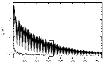
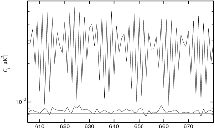
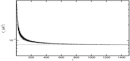
In this study we do not address the question of estimating the noise from the data. Thus, whereas in a more realistic simulation the noise power spectrum to be used for the noise MC simulations would be estimated from the data as discussed above, we have used the same underlying noise power spectrum $P(f)$ for the noise MC simulations as was used for the signal+noise TOD from which we are estimating the $\widehat{C}_{\ell}$. This was a mixture of white and $1/f$ (slope = $-1$) noise with knee frequency $f_{k}=0.1$ Hz. The nominal rms (root-mean-square) level per integration time ($t=1/f_{\mathrm{sample}}=1/108.3$ s) is $\sim 4.8$ mK (thermodynamic temperature scale) for one 100 GHz LFI radiometer. The full set of 24 radiometers at 100 GHz was modelled by reducing this number by a factor of $\sqrt{24}$. We used an SDE (Stochastic Differential Equation) algorithm to generate the TODs of instrumental noise. It is unrealistic to extend the $1/f$ noise spectrum behaviour to very low frequencies. Therefore we have set a minimum frequency $f_{\rm min}=4\times 10^{-6}$ Hz ($\sim(70~{}\hbox{h})^{-1}$) below which the noise spectrum becomes flat. We used $N_{\rm MC}^{\rm(n)}=100$ noise TOD realizations to produce the estimate of $\langle\widetilde{N_{\ell}}\rangle$. According to Balbi et al. (2002), already 22 MC realizations produce a good estimate.

If the instrument noise appears to be non-stationary, SDE can be applied to generate the overall TOD stream in a piecewise manner where each piece is assumed to be stationary with its own specific set of noise model parameter values. The accuracy of the determination of the baseline magnitudes in the destriping is not dependent on whether the noise is stationary throughout the TOD or only piecewise stationary.

Fig. 1 shows the angular power spectrum of the noise map (no destriping) compared with the angular power spectrum after the destriping. Two things are evident. Firstly, without destriping there is a distinct blob structure which is caused by the geometry of the scanning. The amplitudes of the blobs depend on the value of $f_{k}$. The second thing is the significant capacity of the destriping in removing the blobs and making the spectrum approach the spectrum of the white noise. The spectrum deviates from the spectrum of the white noise at low $\ell$. This is an indication that some residual $1/f$ noise remains after the baseline subtraction.

4 Scanning Strategy and Window Function

The order in which the samples of the TOD hit the pixels of the map is determined by the scanning strategy. Therefore any artefacts produced in the maps due to the map-making method can be expected to be affected by the scanning strategy. In this study we used the nominal PLANCK scanning strategy.

In this strategy the spin axis of the satellite follows the ecliptic plane. The spin axis is kept anti-solar by repointing it by $2.5$ arcmin every hour. The spacecraft rotates around the spin axis at a nominal rate of 1 rpm. During one hour PLANCK scans the same circle on the sky 60 times. The scanning pattern used in this study corresponds to the 100 GHz LFI detector number 10 (location $(\theta,\phi)=(3\aas@@fstack{\circ}737,126\aas@@fstack{\circ}228)$ in the focal plane image). The angle between the satellite spin axis and the optical axis of the telescope is $85\degr$. We assumed no spin axis precession. The antenna beam pattern has been modelled by a symmetric Gaussian beam with nominal resolution of FWHM = 10 arcmin (Full Width Half Maximum).

Since we assume idealized satellite motion, where the 60 circles between repointings fall exactly on each other, sample by sample, we can immediately average these circles into a single ring. Thus our simulated TOD consists of 5040 scanning rings, corresponding to 7 months of measurement time, with 6498 samples on each ring, corresponding to a sampling frequency of $f_{\mathrm{sample}}=108.3$ Hz.

The sky coverage of the applied scanning strategy was $f_{\mathrm{sky}}=0.985$, leaving areas close to the poles unobserved. This case is called “nearly full sky” in this paper. In addition, we considered a case called “galactic cut”, where the galactic region ($|b|\leq 20^{\circ}$) is cut out from the maps, leaving $f_{\mathrm{sky}}=0.646$. The numbers of hits in the output map ($N_{\mathrm{side}}=512$) are shown in Fig. 2. The polar regions with no hits and the galactic cut (lower map) are clearly visible. The average number of hits per pixel was $10.6$ in the observed part of the sky (“nearly full sky” case).

Figure 2: The maps with numbers of hits per pixel for the nearly full sky (top) and for the galactic cut (bottom) cases. The maps are in ecliptic coordinate system. Note that the scale is $\log_{10}(\rm{n_{hit}})$, where $\rm{n_{hit}}$ is the number of hits in a pixel.

The window functions $W(\mathbf{n})$ applied in the nearly full sky and in the galactic cut cases were top hat window maps, where each unobserved or cut out pixel was assigned a value zero and for the rest of the pixels value one was assigned. The resolution of the window map was the same as the resolution of our output map. The angular power spectra ($W_{\ell}$) of these window maps were determined with the Anafast code of the HEALPix package. With the aid of the angular spectra the kernel matrices were produced (see Eq. (13)).

5 Filter Function and Signal Bias

Often some kind of filtering is applied to the data to reduce the effect of low-frequency noise. The filtering is applied to the TOD or to the maps. In our case the TOD is “filtered” in a sense that a baseline for each scan circle is subtracted. The magnitudes of the baselines are mainly determined by the $1/f$ noise. However, as described in Section 2 the baseline magnitudes can be influenced by the CMB signal as well and therefore the CMB signal is affected by the baseline subtraction. This effect on the angular power spectrum has to be accounted for. The filter function $F_{\ell}$ was introduced in Eq. (11) as one possible means to model this effect. The filter function will also include the power spectrum distortion caused by any other effects inherent in the map making method.

We determined the filter function $F_{\ell}$ in the following way. Starting from a theoretical input CMB angular power spectrum $C_{\ell}^{\rm th}$ we produced $N_{\rm MC}^{\rm(s)}=450$ pure signal (i.e. no noise) full sky map realizations with $N_{\mathrm{side}}=1024$ by using the Synfast code of the HEALPix package. These maps were then observed using the nominal PLANCK scanning strategy (see Section 4).

The resulting TODs were destriped and coadded into maps. The angular resolution of the crossing point search and the resolution of the output maps were both 7 arcmin (corresponding to $N_{\rm side}=512$). The pseudo angular power spectra ($\widetilde{C}_{\ell}$) were then extracted from the output maps. The $\widetilde{C}_{\ell}$ were also determined from maps with no baselines removed (no destriping). By comparing the filter functions with and without destriping we can distinguish from other effects those filter function contributions which are due to the baseline removal.

The average of these MC realizations, $\langle\widetilde{C}_{\ell}\rangle_{\mathrm{MC}}$, was then used in place of $\langle\widetilde{C}_{\ell}\rangle$ in Eq. (11) and $F_{\ell}$ was solved from this equation (with $\langle\widetilde{N}_{\ell}\rangle=0$).

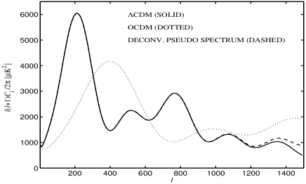
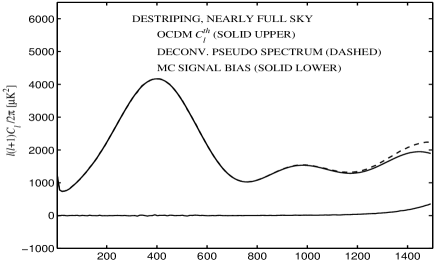
In order to find out whether the filter function $F_{\ell}$ depends on the sky signal we considered two widely different cosmological models: a $\Lambda$CDM (cosmological constant + Cold Dark Matter) model and an open CDM model (OCDM). Their power spectra $C_{\ell}^{\mathrm{th}}$ are depicted in Fig. 3. They were computed from the respective cosmological models by using the Cmbfast code (see Seljak & Zaldarriaga 1996 and references therein). As an example, the ensemble average of a deconvolved pseudo power spectrum $\sum_{\ell^{\prime}}{M_{\ell\ell^{\prime}}^{-1}\langle\widetilde{C}_{\ell^{\prime}}\rangle_{MC}}/B^{2}_{\ell}$ in the case of nearly full sky and $\Lambda$CDM is shown in Fig. 3. The filter function is a ratio of this spectrum and the theoretical power spectrum $C_{\ell}^{\mathrm{th}}$ (compare to Eq. (12)).

Figure 3: The input CMB power spectra $C_{\ell}^{th}$ of the $\Lambda$CDM model (solid curve) and the OCDM model (dotted curve). The ensemble average ($N_{\rm MC}^{\rm(s)}=450$) of the deconvolved pseudo power spectrum from signal-only simulations of the $\Lambda$CDM model is shown as well (dashed curve). The spectrum was derived from the destriped maps and the sky coverage was nearly full sky. The filter function is the ratio of the deconvolved power spectrum (dashed curve) and the input power spectrum (solid curve).

Figure 4: Filter functions $F_{\ell}$ for two widely different input CMB power spectra $C_{\ell}^{th}$. The sky coverage is nearly full sky. The resulting filter functions after the baselines have been removed from the TODs (destriping) are shown. The filter functions are results of $N_{\rm MC}^{\rm(s)}=450$ MC realizations. The filter functions of destriping and no destriping are nearly identical.

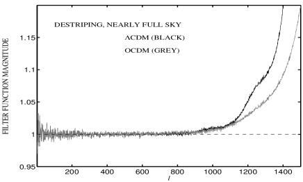
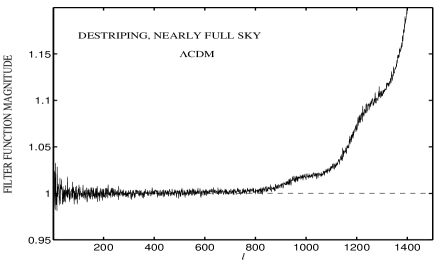
The resulting filter functions with destriping and for the nearly full sky are shown in Fig. 4. (The galactic cut case looks similar, just somewhat noisier.) In order to see in more detail the effect of destriping the ratio between the filter functions with and without destriping were derived. They are shown in Fig. 5. A number of things are evident (see Figs. 4 and 5):

• The filter function stays close to one up to $\ell\simeq$ 700. The deviations from one are completely dominated by remaining cosmic variance (reduced here by $(N_{\mathrm{MC}}^{(s)})^{-1/2}$ due to averaging over $N_{\mathrm{MC}}^{(s)}$ realizations). Thus we conclude that the effect of our map-making method on the angular power spectrum is very small for $l<700$, and we could just use $1$ for the filter function, i.e., no filter function is needed for this part of the spectrum.

• For $l>700$ the filter function deviates from $1$ significantly. This high-$\ell$ tail of the filter function is strongly dependent on $C_{\ell}^{\mathrm{th}}$.

• The filter functions with and without destriping are nearly identical. This shows that the high-$\ell$ tail is caused by some other effects than the baseline removal. The largest relative impact due to baseline removal is around 0.2 per cent (see Fig. 5). The ratio contains blob structure due to low-level stripes introduced by the baseline removal (cf. Fig. 1).

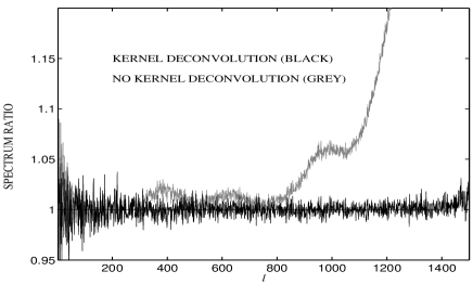
Before drawing further conclusions we need to investigate which part of the high-$\ell$ excess power of the deconvolved pseudo spectrum (see Fig. 3) is caused by numerical errors introduced by the procedures we use for generating sky maps, deriving pseudo spectra from the maps and deconvolving the pseudo spectra with beam, pixel weight and mode-mode coupling kernel matrix ($M_{\ell\ell^{\prime}}$). For that purpose we produced 100 realizations of the full sky CMB maps from the $\Lambda$CDM input power spectrum, applied our “galactic cut” window function, and determined the pseudo spectra of the resulting maps. The mean of these pseudo spectra was then deconvolved with the beam, with the pixel weight (provided by HEALPix package) and with the kernel matrix. The resulting deconvolved spectrum had a close resemblance to the theoretical input spectrum $C_{\ell}^{th}$. Their ratio is depicted in Fig. 6 (black curve). The ratio stays close to one at all multipoles considered, showing that the procedures we use for the generation of sky maps and pseudo spectra and for the deconvolution are not responsible for the high-$\ell$ tail of the filter function (shown in Fig. 4).

Figure 5: The ratio between filter functions with and without destriping. Nearly full sky coverage and $\Lambda$CDM cosmological model were applied. Note that different panels show the ratio at different ranges of $\ell$.

Figure 6: CMB power spectra were produced by first generating 100 realizations of the full sky, then cutting out part of the observations (galactic cut case, see Fig. 2), then taking the mean of the pseudo power spectra derived from the partial sky maps and finally deconvolving the mean with beam, pixel weight and kernel matrix. The ratio between the deconvolved spectrum and the theoretical input spectrum $C_{\ell}^{th}$ is shown (black curve). The ratio without deconvolution with the kernel matrix is demonstrated as well (grey curve). The cosmological model was $\Lambda$CDM. All maps had $N_{\mathrm{side}}=512$.

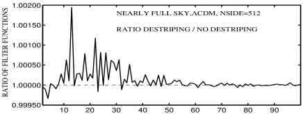
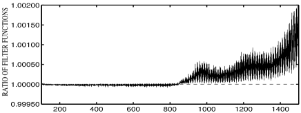
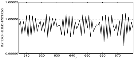
The dependence of the filter function on $C_{\ell}^{\mathrm{th}}$ (see Fig. 4) shows that it is not a good way to model the effect of our map-making method. That the effect appears at high $\ell$ suggests that it might be related to the pixel size used. Therefore we determined the filter functions also for map resolutions $N_{\mathrm{side}}=2048$ (sky map) and $N_{\mathrm{side}}=1024$ (output map). Results are shown in Fig. 7: a high-$\ell$ tail still exists, and is in fact somewhat higher than in the earlier case of $N_{\mathrm{side}}=512$ (output map). Thus the filter function tail cannot be removed simply by increasing the map resolution. (Note that the $N_{\mathrm{side}}=512$ pixel size is about 7 arcmin and should thus resolve the power spectrum up to $\ell\sim 180^{\circ}/7~{}\hbox{arcmin}\sim 1500$.)

Figure 7: Same as Fig. 4 but now the sky map realizations (scanned for TOD) and the output map had higher resolutions ($N_{\mathrm{side}}=2048$ and $N_{\mathrm{side}}=1024$, respectively). The filter function is a result of $N_{\rm MC}^{\rm(s)}=450$ MC realizations.

The binning of the detector pointings in pixels has been treated in time domain by Doré et al. (2001). In a noise-free experiment they considered a residual between an observed TOD and another TOD produced by scanning a pixelized map that is naively coadded from the observed TOD. This residual was called pixelization noise.

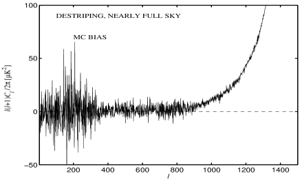
We have determined (Appendix A) that the main effect causing the high-$\ell$ tail of the filter function is related to the distribution of the detector pointings on the sky and its relation to the pixelization. Comparing the filter functions of the $\Lambda$CDM and OCDM cases to the corresponding $C_{\ell}^{\mathrm{th}}$ one notices that they appear to be inversely related. Since the filter function is essentially a ratio between $\langle\widehat{C}_{\ell}\rangle$ and $C_{\ell}^{\mathrm{th}}$, this suggests that the dominant contribution would be better modelled as an offset $S_{\ell}$, which we call signal bias,

$$\langle\widetilde{C}_{\ell}\rangle=\sum_{\ell^{\prime}}M_{\ell\ell^{\prime}}B_{\ell^{\prime}}^{2}C_{\ell^{\prime}}^{th}+S_{\ell}+\langle\widetilde{N}_{\ell}\rangle\,.$$ (14)

It can be estimated by signal-only MC simulations just like the filter function. An equation similar to Eq. (12) can be written for the estimate of $C_{\ell}^{th}$,

$$\widehat{C}_{\ell}=\frac{\sum_{\ell^{\prime}}{M_{\ell\ell^{\prime}}^{-1}\left(\widetilde{C}_{\ell^{\prime}}-S_{\ell^{\prime}}-\langle\widetilde{N}_{\ell^{\prime}}\rangle\right)}}{B^{2}_{\ell}}.$$ (15)

The average pseudo power spectrum of the MC realizations, $\langle\widetilde{C}_{\ell}\rangle_{\mathrm{MC}}$, can be used in place of $\langle\widetilde{C}_{\ell}\rangle$ in Eq. (14) and $S_{\ell}^{\mathrm{MC}}$ can be solved from this equation, with $\langle\widetilde{N}_{\ell}\rangle=0$.

Further details of the signal bias are derived in Appendix A. It is shown there that the signal bias estimates are rather similar even though the cosmological models are widely different.

The signal bias is reduced when data from several detectors are combined, since that increases the density of detector pointings. We find in Appendix A that the signal bias in the region of high $\ell$ is nearly inversely proportional to the number of detectors. In reality, the detector pointings from successive scan circles also do not fall exactly on top of each other. Therefore, in the case of the real PLANCK experiment this signal bias may be small enough (when compared to other systematic effects) to be ignored.

In our idealized simulation, which utilizes only pointings of a single detector and assumes exact overlap of successive scan circles within the same pointing period, the signal bias is larger, and shows up prominently in our results. For comparing the signal bias to other map-making artefacts we carried out destriping on a noiseless TOD containing CMB and galactic foreground signals. In this case the signal bias was significantly larger (close to two orders of magnitude larger at high $\ell$) than the residual power spectrum due to the subtracted baselines.

We show in Appendix A that the signal bias can be reliably estimated by MC simulation and thus removed. We have done this in what follows.

6 Analysis Pipeline and Computing Time

The starting point for our analysis is a TOD with CMB+noise (the “original TOD”), and a noise power spectrum $P(f)$. Our analysis pipeline is composed of the following steps:

1. A total of $N_{\rm MC}^{(\rm n)}$ pure noise TODs are produced, using $P(f)$. They are destriped and maps are coadded from the TODs from which the baselines have been removed. The angular power spectra of the output maps are produced with the Anafast code. By averaging the obtained spectra an estimate for $\langle\widetilde{N}_{\ell}\rangle$ is obtained.

2. From the original TOD a destriped map is produced, from which a power spectrum estimate $\widehat{C}^{\prime}_{\ell}$ is obtained, using Eq. (15) with $S_{\ell}=0$.

3. Random generation of $N_{\rm MC}^{(\rm s)}$ pure CMB sky realizations with the Synfast code. The estimate $\widehat{C}^{\prime}_{\ell}$ is used as an input power spectrum. In order to produce a TOD, the sky is observed according to the selected scanning strategy. TODs are destriped and projected back onto the sky. The maps are input to Anafast for the determination of their angular power spectra. These spectra are used for determining the signal bias $S_{\ell}^{\mathrm{MC}}$.

4. The power spectrum estimate $\widehat{C}_{\ell}$ is obtained, using Eq. (15) with $S_{\ell}^{\mathrm{MC}}$.

At this point we have our final power spectrum estimate $\widehat{C}_{\ell}$. To obtain an estimate for the error bars and the covariance matrix, further simulations are required. In the case of a real experiment, these simulations would be based on the $\widehat{C}_{\ell}$ just obtained. However, in this study we have also available the $C_{\ell}^{\mathrm{th}}$ used to produce the original TOD. The emphasis of this study is to reveal the actual error bars of our method, rather than to simulate the estimation of these error bars in a real experiment. Thus we use this $C_{\ell}^{\mathrm{th}}$ as the input spectrum to generate an ensemble of MC estimates $\widehat{C}_{\ell}$.

1. A total of $N_{\rm MC}^{(\rm{s+n})}$ randomly generated “experimental” TODs (i.e. with sky signal and noise) are produced. They are destriped and coadded into a map. Thereafter the pseudo power spectra $\widetilde{C}_{\ell}$ are determined.

2. The estimated angular power spectra $\widehat{C}_{\ell}$ are computed using Eq. (15) and binned.

3. The $\pm 1\sigma$ error bars on each $\widehat{C}_{\ell}$ and bin are evaluated as std (standard deviation) calculated over the MC realizations.

In our simulations we had $N_{\rm MC}^{(\rm n)}=100$, $N_{\rm MC}^{(\rm s)}=450$, and $N_{\rm MC}^{(\rm{s+n})}=450$. The relatively large number of signal+noise MC cycles was required to study the statistics of the $\widehat{C}_{\ell}$ estimates. The relative rms accuracy of the $\pm 1\sigma$ error bars is $(2N_{\rm MC}^{(\rm{s+n})})^{-1/2}$. With $N_{\rm MC}^{(\rm{s+n})}=450$ this implies 3.3 per cent rms accuracy. Additionally, this number of MC realizations is high enough to reveal some features of the covariance matrix $\widehat{C}_{\ell\ell^{\prime}}=\langle(\widehat{C}_{\ell}-\langle\widehat{C}_{\ell}\rangle)(\widehat{C}_{\ell^{\prime}}-\langle\widehat{C}_{\ell^{\prime}}\rangle)\rangle$ (Section 7). However, to obtain estimates for individual off-diagonal elements of $\widehat{C}_{\ell\ell^{\prime}}$, or even of the binned covariance matrix $\widehat{\mathcal{C}}_{bb^{\prime}}=\langle(\widehat{\mathcal{C}}_{b}-\langle\widehat{\mathcal{C}}_{b}\rangle)(\widehat{\mathcal{C}}_{b^{\prime}}-\langle\widehat{\mathcal{C}}_{b^{\prime}}\rangle)\rangle$ would have required an even larger $N_{\rm MC}^{(\rm{s+n})}$. For $N_{\rm MC}^{(\rm{s+n})}=450$ the off-diagonal elements were still dominated by MC noise for bins of $\Delta\ell=10$.

As for the original MASTER approach, our pipeline is well parallelisable in the sense that each MC cycle can be run in its own CPU. This allows for a linear scaling with the number of CPUs and with the number of MC cycles performed. In our pipeline the most CPU time consuming step is the SDE noise generation. In an AIX IBM pSeries690 machine with Power4 processor running at clock speed of 1.1 GHz it takes $\sim 1$ h on a single processor to produce one noise TOD for a single detector with length corresponding to 7 months of mission time ($\sim 2\times 10^{9}$ samples). We have also implemented a parallel version of the SDE code which brings the required time to generate one noise TOD down to $\sim 9$ min with 14 processors.

Destriping and map coaddition of one 7 month TOD will take $\sim 50$ s of CPU time in a single processor serial job.

7 Simulations and Results

To test our joint destriping and MASTER approach in the estimation of the angular power spectra we considered simulations relevant for the 100 GHz channels originally planned for the LFI instrument on-board the PLANCK satellite. The simulations included CMB sky and instrument noise realizations. The applied signal+noise simulation procedure was described in Section 6.

The scanning strategy, antenna beam response and the instrument noise characteristics applied in the simulations were those described in Sections 3.2 and  5. When the noise TODs were generated the effect of using the full set of 24 radiometers was modelled as described in Section 3.2. When the signal TODs were generated a single detector scanning was assumed.

Figure 8: Top panel: Output map without destriping. Bottom panel: Output map after destriping.

Figure 9: Top panel: Noise-only output map without destriping. Bottom panel: Noise-only output map after destriping.

Figure 10: Top panel shows the noisy power spectrum estimate (solid curve) used as an input spectrum to the signal-only MC to determine the estimate for the signal bias. The true $C_{\ell}^{\mathrm{th}}$ is shown as well ($\Lambda$CDM, dashed curve). Bottom panel shows the obtained signal bias estimate. The sky coverage is nearly full sky.

Figure 11: CMB power spectrum estimated by using the destriping technique and MASTER approach for the 100 GHz channels of PLANCK LFI. The use of 24 radiometers has been modelled by dividing the rms white noise level of a single detector with a factor $\sqrt{24}$. Nearly full sky has been observed. Top panel shows the power spectra obtained for a single sky and noise realization: pseudo power spectrum $\widetilde{C}_{\ell}$ - grey points, the estimated power spectrum of the noise - dashed line, the estimate of the CMB power spectrum $\widehat{C}_{\ell}$ - black points, and the input power spectrum of the true sky $C_{\ell}^{th}$ - solid line. Bottom panel shows the estimate (midpoints of the error bars) of the CMB power spectrum in bins of 10. The error bars are derived from $N_{\rm MC}^{(\rm{s+n})}=450$ MC realizations of signal and noise. The solid line is the input power spectrum. The magnitudes of the error bars are $\pm 1\sigma$. For clarity, only the odd bins are shown.

Figure 12: Same as Fig. 11, except that the galactic region with $|b|\leq 20^{\circ}$ has been cut out from the observations.

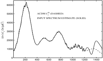
The angular power spectrum $C_{\ell}^{th}$ of the $\Lambda$CDM cosmological model was used as the input spectrum in the signal+noise simulations. The applied input spectrum is depicted in Fig. 3.

Fig. 8 shows a map produced from a simulated CMB+noise TOD, both before and after destriping. Fig. 9 shows the same for a pure noise TOD.

7.1 Power Spectrum Estimate

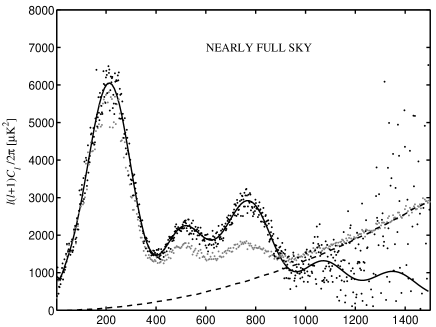
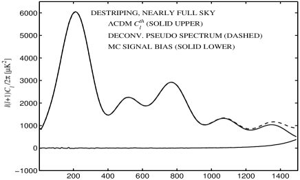
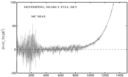
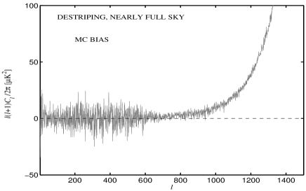
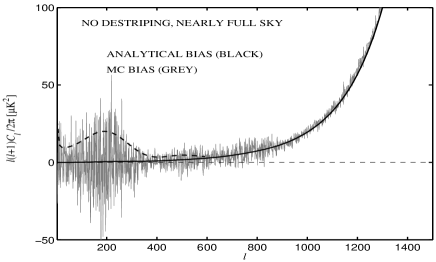
The power spectrum estimates $\widehat{C}_{\ell}$ were solved from Eq. (15). In a real CMB experiment we will not have the true angular power spectrum $C_{\ell}^{th}$ available for generating the signal bias estimate $S_{\ell}^{\rm{MC}}$. Instead a noisy power spectrum estimate can be utilized as described in Section 6. The power spectrum estimate and the signal bias for nearly full sky are shown in Fig. 10. The signal bias for the galactic cut can be obtained similarly. The applied noise bias $\langle\widetilde{N}_{\ell}\rangle$ is depicted in the bottom panel of Fig. 1 (nearly full sky). The kernel matrices ($M_{\ell\ell^{\prime}}$) derived in Section 5 were applied.

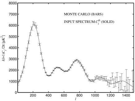
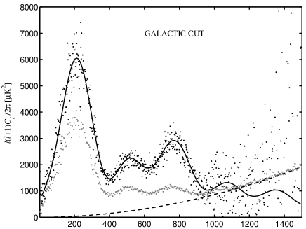
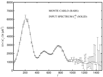
The resulting angular power spectrum estimates and the corresponding $\pm 1\sigma$ error bars are shown in Figs. 11 and 12 for the nearly full sky and for the cut sky cases, respectively. Individual $\widehat{C}_{\ell}$ are dominated by the instrument noise for $\ell>1000$.

Figure 13: In order to reveal the possible bias in our method, we show the relative differences (thicker step curve) between the mean binned power spectrum estimate $\langle\widehat{\mathcal{C}}_{b}\rangle_{\rm MC}$ (from $N_{\rm MC}^{(\rm{s+n})}=450$ MC realizations of signal and noise) and the binned input power spectrum $\mathcal{C}_{b}^{\rm th}$ representing the underlying theoretical spectrum. The y axis quantity is $(\langle\widehat{\mathcal{C}}_{b}\rangle_{\rm MC}-\mathcal{C}_{b}^{\rm th})/\mathcal{C}_{b}^{\rm th}$. The results of the nearly full sky are shown. The symmetric smooth curves show the $\pm\sigma_{o}$ limits, where $\sigma_{o}=\Delta_{\rm ref}\widehat{\mathcal{C}}_{b}/(\mathcal{C}_{b}^{th}(N_{\rm MC}^{(\rm{s+n})})^{1/2})$ is the “expected” standard deviation from MC noise (the reference value from Eq. (19)). No obvious bias is seen. The thinner step curve shows the situation without accounting for the signal bias. In this case there is a clear positive bias for larger $\ell$.

Figure 14: Same as Fig. 13 but now the galactic region is cut out from the output maps.

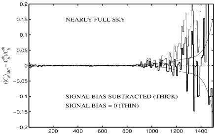
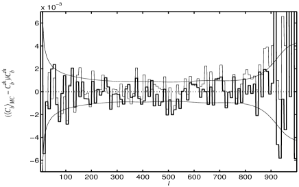
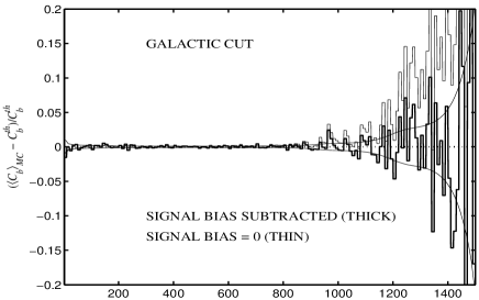
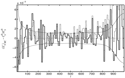
The bottom panels of Figs. 11 and 12 show the estimates

$$\widehat{\mathcal{C}}_{b}=\sum_{\ell\in b}{\frac{\ell(\ell+1)\widehat{C}_{\ell}}{2\pi\Delta\ell}},$$ (16)

of the CMB angular power spectrum in bins $b$ of $\Delta\ell=10$. The error bars (bottom panels) were determined from the MC variance of the binned power spectrum estimates. The good match between the estimated and the input power spectra shows that the combined destriping and MASTER approach produces power spectrum estimates with good accuracy.

In order to examine the possible bias in our angular power spectrum estimates the mean $\langle\widehat{\mathcal{C}}_{b}\rangle_{\rm MC}$ of the $\widehat{\mathcal{C}}_{b}$ spectra available from our MC realizations was determined. The relative differences $(\langle\widehat{\mathcal{C}}_{b}\rangle_{\rm MC}-\mathcal{C}_{b}^{\rm th})/\mathcal{C}_{b}^{\rm th}$ are shown in Figs. 13 and 14.

The signal bias and the power spectrum estimates will be correlated if the same seed values are used when the random sky realizations are generated in the signal-only and in the signal+noise simulations. This could lead to too optimistic results. We intentionally used different seed values between the signal-only and the signal+noise simulations.

It is evident from Figs. 13 and 14 that no systematic bias can be observed and the variation from bin-to-bin is mainly caused by the residual cosmic variance and the instrument noise that remain after the averaging. If any bias exists its relative level is at most of the order of 0.1 per cent for $\ell<800$.

If we had not accounted for the signal bias our method would have produced biased estimates. To see how large is the effect we did the same analysis, keeping $S_{\ell}=0$. This case is shown in Figs. 13 and 14 as well. A clear bias at high $\ell$ ($\ell>1000$) can be detected.

7.2 Covariance Matrix and Statistics

Figure 15: The diagonals $\widehat{C}_{\ell,\ell+1}\ldots\widehat{C}_{\ell,\ell+6}$ of the covariance matrix are shown from top down. The matrix is normalized to $\widehat{C}_{\ell\ell}=1$. The expected std of the MC noise of the off-diagonals is $(N_{MC})^{-1/2}=0.047$, where $N_{MC}=450$. The std of the diagonals shown in the figure vary in the range 0.046 …0.050. Note that the levels of the diagonals $\widehat{C}_{\ell,\ell+2}$ and $\widehat{C}_{\ell,\ell+4}$ are systematically negative. The values of $\widehat{C}_{\ell,\ell+2}$ seem to increase with increasing $\ell$. The sky coverage is galactic cut.

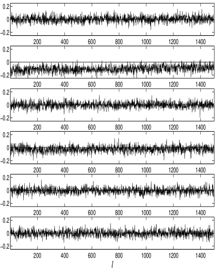
The covariance matrix of the power spectrum estimates was determined from the $N_{\rm{MC}}=450$ signal+noise MC realizations. The elements of the matrix are $\widehat{C}_{\ell\ell^{\prime}}=\langle(\widehat{C}_{\ell}-\langle\widehat{C}_{\ell}\rangle_{\rm{MC}})(\widehat{C}_{\ell^{\prime}}-\langle\widehat{C}_{\ell^{\prime}}\rangle_{\rm{MC}})\rangle_{\rm{MC}}$. The diagonals $\widehat{C}_{\ell,\ell+1}\ldots\widehat{C}_{\ell,\ell+6}$ from the upper right triangle are shown in Fig. 15 (galactic cut). Before plotting, the covariance matrix was normalized,

$$\widehat{C}_{\ell\ell^{\prime}}^{\rm{norm}}=\frac{\widehat{C}_{\ell\ell^{\prime}}}{\sqrt{\widehat{C}_{\ell\ell}}\sqrt{\widehat{C}_{\ell^{\prime}\ell^{\prime}}}}.$$ (17)

to make all the main diagonal elements equal to one. The $\ell$-to-$\ell$ variation of the off-diagonals is mainly caused by the MC noise.

The second and the fourth diagonals are mostly negative. Their mean (up to $\ell=800$) values are -0.116 and -0.0265, respectively. No level shift can be detected in the sixth or higher even diagonals. Excluding the diagonals $\widehat{C}_{\ell,\ell\pm 2}$ and $\widehat{C}_{\ell,\ell\pm 4}$ the elements of the rest of the covariance matrix were buried under the MC noise. An analytical model for the covariance matrix $\widehat{C}_{\ell\ell^{\prime}}$ of the pseudo-$C_{\ell}$ estimators exists (Efstathiou, 2003). In the CMB dominated region (below $\ell\simeq 800$) it forecasts for the mean levels of the second and the fourth diagonals -0.113 and -0.0266, respectively. The good match between the model values and the values obtained from the MC realizations is notable. The same model gives mean values around $-1\times 10^{-4}$ for the rest of the diagonals shown in Fig. 15. No level shifts that would stand out from the MC noise could be detected in the covariance matrix of the nearly full sky.

Figure 16: The ratios of the variances $\Delta^{2}_{\rm{MC}}\widehat{C}_{\ell}/\Delta^{2}_{\rm{ref}}\widehat{C}_{\ell}$ (top panel) and $\Delta^{2}_{\rm{MC}}\widehat{\mathcal{C}}_{b}/\Delta^{2}_{\rm{ref}}\widehat{\mathcal{C}}_{b}$ (bottom panel). $\Delta^{2}_{\rm{MC}}$ refers to the MC variance and $\Delta^{2}_{\rm{ref}}$ is the reference value defined in Eqs. (18) and (19). In Eq. (18) the quantity $\langle\widetilde{N}_{\ell}\rangle_{\rm{MC}}$ obtained from $N_{\rm MC}^{(\rm n)}=100$ noise-only MC realizations was used instead of $\langle\widetilde{N}_{\ell}\rangle$. The number of signal+noise MC realizations was 450 when determining the variances. The horizontal lines in the top panel were derived from the analytical model of the covariance matrix of the power spectrum estimates (Efstathiou, 2003).

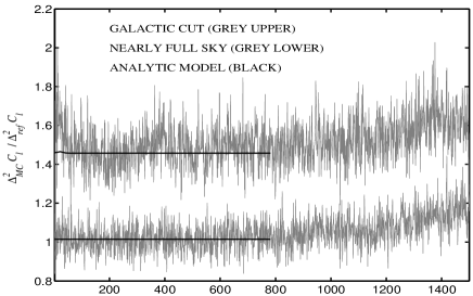
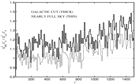
The theoretical variance for the full-sky case is given by Eq. (9). For the cut sky less information is available, which increases the variance. The cut sky also introduces correlations between the estimates $\widehat{C}_{\ell}$. The binned values $\widehat{\mathcal{C}}_{b}$ should be less correlated. According to a “rule of thumb” (for bins $\widehat{\mathcal{C}}_{b}$) the variance should be larger approximately by a factor $1/f_{\rm sky}$ (e.g. Scott, Srednicki & White, 1994; Hobson & Magueijo, 1996). Thus we shall use as reference values for the variances

$$\Delta_{\rm ref}\widehat{C}_{\ell}=\sqrt{\frac{2}{(2\ell+1)f_{\rm sky}}}\bigg{(}C_{\ell}^{th}+{}$$

$$+{}\frac{\sum_{\ell^{\prime}}{M_{\ell\ell^{\prime}}^{-1}(S_{\ell^{\prime}}+\langle\widetilde{N}_{\ell^{\prime}}\rangle})}{B_{\ell}^{2}}\bigg{)}$$ (18)

and

$$\Delta^{2}_{\rm ref}\widehat{\mathcal{C}}_{b}=\frac{1}{{\Delta\ell}^{2}}\sum_{\ell\in b}{\left(\frac{\ell(\ell+1)\Delta_{\rm ref}\widehat{C}_{\ell}}{2\pi}\right)^{2}}.$$ (19)

We show the ratios of the MC variances from our simulations to these reference values, $\Delta^{2}_{\rm{MC}}\widehat{C}_{\ell}/\Delta^{2}_{\rm{ref}}\widehat{C}_{\ell}$ and $\Delta^{2}_{\rm{MC}}\widehat{\mathcal{C}}_{b}/\Delta^{2}_{\rm{ref}}\widehat{\mathcal{C}}_{b}$, in Fig. 16.

The top panel of Fig. 16 shows that the MC variance of the unbinned power spectrum estimate is larger than its reference value. Lowering the sky coverage will produce a larger ratio. The ratio remains relatively flat up to $\ell\approx 1200$. At higher $\ell$ a positive bump appears. The horizontal solid lines indicate the expected levels derived from the analytical model of the covariance matrix $\widehat{C}_{\ell\ell^{\prime}}$ (Efstathiou, 2003). The model is valid in the CMB dominated region. In the nearly full sky coverage the MC variances follow closely the model variances. In the galactic cut the model is valid only at high enough $\ell$ (above $\ell\simeq 5$). The MC variances of the galactic cut are in average slightly larger than the model variances. The mean relative difference is 1.8 per cent.

The ratios between the MC variances of the binned estimates and their reference values are shown in the bottom panel of Fig. 16. Since the estimates at $\ell$ and $\ell+2$ are anticorrelated, binning them into the same bin reduces the variance by more than $\Delta\ell$. The less correlated the bins are, the closer to the reference value (Eq. (19)) we expect their variance to be. A smaller sky coverage implies more correlation and thus a higher excess variance. For our cut sky the remaining excess variance is 10 …20 per cent for bins of $\Delta\ell=10$ up to $\ell\sim 1000$. For nearly full sky no excess variance is seen below $\ell=800$. For larger $\ell$ there is more excess variance. This happens when the spectrum becomes noise dominated.

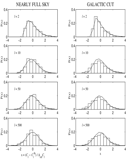
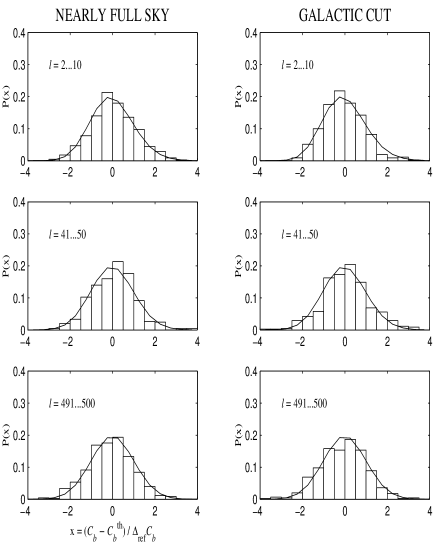
We determined also the statistical distributions of the angular power spectrum estimates obtained with our $C_{\ell}$ estimation technique. Examples of the PDFs (Probability Density Function) of the unbinned ($\widehat{C}_{\ell}$) and the binned ($\widehat{\mathcal{C}}_{b}$) estimates are shown in Figs. 17 and 18. These PDFs were compared to the PDFs of a central $\chi^{2}_{\nu}$ model (also shown). The match between the MC PDFs and the model PDFs is good in the case of nearly full sky coverage. In the galactic cut the match is poorer especially in the PDFs of the unbinned estimates. This is as expected, since the degrees of freedom ($\nu$) in the model PDFs were determined from the formula $\nu=(2\ell+1)f_{\rm sky}$, which is just a ”rule of thumb” approximation in the galactic cut case, and does not correctly take into account the correlation between nearby $\widehat{C}_{\ell}$. The obtained PDFs confirm the earlier finding that the deviation of the MC variance from its reference value becomes larger when the sky coverage fraction is lowered (see Fig. 16).

Figure 17: PDFs $P(x)$ of $\widehat{C}_{\ell}$ for some selected multipoles $\ell$. The bars are histograms derived from 450 signal+noise MC realizations. The solid curves are the PDFs from the central $\chi_{\nu}^{2}$ model with $\nu=(2\ell+1)f_{\rm sky}$. The std of the model is set to $\Delta_{\rm{ref}}\widehat{C}_{\ell}$, which is the reference value of the std of $\widehat{C}_{\ell}$ defined in Eq. (18). In the plot the x axis quantity of the model PDF is first normalized with $\Delta_{\rm{ref}}\widehat{C}_{\ell}$ and then the PDF is shifted along the x axis so that its expectation value will coincide with $x=0$.

Figure 18: Same as Fig. 17 but now the PDFs are for the binned estimates $\widehat{\mathcal{C}}_{b}$. In the central $\chi_{\nu}^{2}$ model the number of degrees of freedom is set to $\nu=\sum_{\ell\in b}{(2\ell+1)f_{\rm sky}}$. The std of the model is set to $\Delta_{\rm{ref}}\widehat{\mathcal{C}}_{b}$. The bin size is $\Delta\ell=10.$

8 Conclusion

We have demonstrated that the combination of destriping technique and our MASTER approach can tackle the extraction of the CMB angular power spectra. The approach was found to work well yielding accurate estimates of the true power spectrum of the sky. As a practical example, we considered the 100 GHz channels of the LFI instrument of the PLANCK satellite.

Destriping as a map-making method is general in a sense that it requires no prior information either on the instrument noise properties or on the actual beam shape. We can expect that even in the case of non-stationary noise we are able to recover the baseline magnitudes accurately. The MASTER technique requires knowledge of the noise characteristics. In realistic CMB experiments the noise parameters need to be estimated from the measured data. However, we did not address the noise estimation techniques in this study. Thus the correct instrument noise model was assumed throughout this paper.

We found that the effect of the sky signal on destriping does not cause a significant distortion on the power spectrum estimates. Therefore no filter function is needed to compensate for it.

Instead we discovered an effect related to the clustering of the detector pointings. Because of the high stability of the motion of the PLANCK satellite the centre points of the measurements taken during the 1 h period between satellite spin-axis repointings form tight clusters of 60. In our idealized simulation these were all assumed to fall on a single point, which exaggerates the effect somewhat. This leads to a noticeable effect at high $\ell$ (for $\ell>700$ in our simulations). We were able to account for this effect, and remove it, by introducing the concept of signal bias in the $C_{\ell}$ estimate, and determining it by signal-only MC simulations. We also derived a reasonably accurate analytical estimate for the signal bias.

It was shown that the signal bias will be reduced when data from several detectors are combined, since that increases the density of detector pointings. In addition, due to satellite spin axis nutation (amplitudes up to 1.5 arcmin, van Leeuwen et al. 2002) and spin rate variation the detector pointings from successive scan circles will not fall exactly on top of each other, in reality. Therefore, in the case of the real PLANCK experiment this signal bias may be small enough to be ignored.

An ensemble of angular power spectrum estimates were produced by applying our estimation method to the maps of the signal+noise MC realizations. Our results showed that, after removing the signal and noise biases, any remaining bias was buried under the MC variations; if any bias exists its relative level was not higher than 0.1 per cent.

There was a good match between the $\pm 1\sigma$ error bars obtained from the MC realizations and derived from the analytical model of the pseudo-$C_{\ell}$ estimators (Efstathiou, 2003). This indicates that the implementation related performance losses of our method are small.

Appendix A Signal Bias

In our signal-only simulations (Section 5) we noted an effect (at high $\ell$) in the angular power spectra of the output maps, that was not explained by beam size, pixel size, or window function, and could not properly be modelled in terms of a filter function. We studied this effect in detail, and conclude that

1. The effect can be modelled as an offset $S_{\ell}$, which we call signal bias.

2. The effect is due to the resolution by which the sky is sampled by the detector pointings.

Since in the realistic PLANCK experiment the effect will be less important than in our idealized simulation, we have relegated the detailed discussion of this effect in this Appendix.

We pick up the discussion from Section 5, where we introduced the signal bias in Eq. (14), reproduced here:

$$\langle\widetilde{C}_{\ell}\rangle=\sum_{\ell^{\prime}}M_{\ell\ell^{\prime}}B_{\ell^{\prime}}^{2}C_{\ell^{\prime}}^{th}+S_{\ell}+\langle\widetilde{N}_{\ell}\rangle\,.$$ (20)

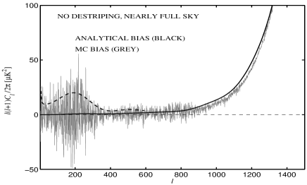
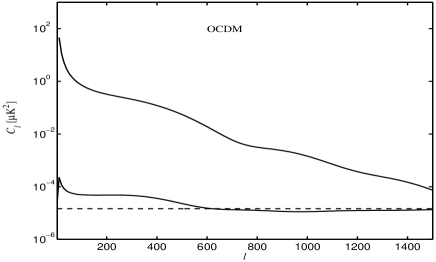
The mean pseudo spectra ($\langle\widetilde{C_{\ell}}\rangle_{\rm{MC}}$) obtained in Section 5 were inserted in Eq. (20) and the deconvolved signal bias estimate $\sum_{\ell^{\prime}}{M_{\ell\ell^{\prime}}^{-1}S_{\ell^{\prime}}^{\mathrm{MC}}}/B^{2}_{\ell}$ was solved (with $\langle\widetilde{N_{\ell}}\rangle=0$). It is shown in Fig. 19 for the $\Lambda$CDM model and for the nearly full sky. Fig. 20 depicts similar things for the OCDM case. The galactic cut cases look similar but somewhat noisier. The signal bias estimates have a remarkable resemblance even though the cosmological models are widely different. This indicates that the signal bias approach is much better suited to our map-making method than the filter function.

A.1 Pointing Distribution

Let us consider CMB only (no noise) and assume no baseline removal for the time being. Let $k$ index the pixels of the final output map. As a result of averaging the observations the output map pixel temperature $\widetilde{T}_{k}$ of pixel $k$ is

$$\widetilde{T}_{k}=\frac{1}{p_{k}}\sum_{i=1}^{p_{k}}T_{ik},$$ (21)

where $p_{k}$ is the number of hits in pixel $k$, $i$ indexes a hit in pixel $k$ and $T_{ik}$ is the observed sky temperature of hit $i$. The pixel temperature $\widetilde{T}_{k}$ can be written as

$$\widetilde{T}_{k}=T_{k}+\widetilde{T}_{k}-T_{k}=T_{k}+\Delta T_{k}\,,$$ (22)

where $T_{k}$ is the beam and pixel smoothed sky temperature of pixel $k$. The temperatures $T_{k}$ and $T_{ik}$ can be given in terms of the expansion coefficients $a_{\ell m}$ (see Eq. (1))

$$T_{k}=\sum_{\ell m}a_{\ell m}B_{\ell}Y_{\ell m}(\mathbf{n}_{k})$$ (23)

and

$$T_{ik}=\sum_{\ell m}a_{\ell m}B^{\prime}_{\ell}Y_{\ell m}(\mathbf{n}_{ik}),$$ (24)

where $B^{\prime}_{\ell}$ contains the beam and pixel smoothing of the sky map and $B_{\ell}$ contains the same for the output map. $\mathbf{n}_{k}$ is a unit vector pointing to the center of the pixel $k$. $\mathbf{n}_{ik}$ is a unit vector of the pointing of the observation $i$ in pixel $k$. Performing the reverse spherical transform to both sides of Eq. (22) one obtains a relation for the expansion coefficients

$$\Omega_{p}\sum_{k}\widetilde{T}_{k}Y_{\ell m}^{\star}(\mathbf{n}_{k})=\Omega_{p}\sum_{k}T_{k}Y_{\ell m}^{\star}(\mathbf{n}_{k})+$$

$$+\Omega_{p}\sum_{k}\Delta T_{k}Y_{\ell m}^{\star}(\mathbf{n}_{k}),$$ (25)

where only the hit pixels will be included in the sums.

Figure 19: Top panel: Mean deconvolved pseudo power spectrum $\sum_{\ell^{\prime}}{M_{\ell\ell^{\prime}}^{-1}\langle\widetilde{C}_{\ell^{\prime}}\rangle_{\mathrm{MC}}}/B^{2}_{\ell}$ (dashed curve), $\Lambda$CDM input spectrum $C_{\ell}^{th}$ (solid upper curve) and deconvolved signal bias estimate (difference of those two, solid lower curve). Destriping has been applied in the map-making stage. Middle panel: Deconvolved signal bias estimate shown with expanded y-scale. Bottom panel: Deconvolved signal bias estimate when no baseline removal has been performed (no destriping). Also shown are the deconvolved analytical approximation, Eq. (41), of the signal bias $S_{\ell}^{app}$ (black curve) and the reference value $\Delta_{\rm ref}\widehat{C}_{\ell}$ divided by $(N_{\rm MC}^{\rm(s)})^{1/2}$ (dashed curve), where $N_{\rm MC}^{\rm(s)}=450$ is the number of MC realizations to produce $\langle\widetilde{C}_{\ell}\rangle_{\mathrm{MC}}$.

Figure 20: Same as Fig. 19 (two upper panels) but now the cosmological model is OCDM.

The ensemble mean of the pseudo power spectrum $\widetilde{C}_{\ell}$ can be obtained as

$$\langle\widetilde{C}_{\ell}\rangle=\frac{1}{2\ell+1}\sum_{m=-\ell}^{\ell}\langle|\Omega_{p}\sum_{k}\widetilde{T}_{k}Y_{\ell m}^{\star}(\mathbf{n}_{k})|^{2}\rangle.$$ (26)

As a consequence of Eq. (25) the mean can be split in three terms

$$\langle\widetilde{C}_{\ell}\rangle=\langle C_{\ell}^{x}\rangle+\langle C_{\ell}^{\Delta}\rangle+\langle C_{\ell}^{x\Delta}\rangle$$ (27)

with the following formulas

$$\langle C_{\ell}^{x}\rangle\!\! = \!\!\frac{\Omega_{p}^{2}}{2\ell+1}\sum_{m=-\ell}^{\ell}\sum_{k,p}\langle T_{k}T_{p}^{\star}\rangle Y_{\ell m}^{\star}(\mathbf{n}_{k})Y_{\ell m}(\mathbf{n}_{p})\,,$$ (28)

$$\langle C_{\ell}^{\Delta}\rangle\!\! = \!\!\frac{\Omega_{p}^{2}}{2\ell+1}\sum_{m=-\ell}^{\ell}\sum_{k,p}\langle\Delta T_{k}\Delta T_{p}^{\star}\rangle Y_{\ell m}^{\star}(\mathbf{n}_{k})Y_{\ell m}(\mathbf{n}_{p})$$ (29)

and

$$\langle C_{\ell}^{x\Delta}\rangle=\frac{\Omega_{p}^{2}}{2\ell+1}\sum_{m=-\ell}^{\ell}\sum_{k,p}\big{(}\langle T_{k}\Delta T_{p}^{\star}\rangle Y_{\ell m}^{\star}(\mathbf{n}_{k})Y_{\ell m}(\mathbf{n}_{p})+{}$$

$${}+\langle T_{k}^{\star}\Delta T_{p}\rangle Y_{\ell m}(\mathbf{n}_{k})Y_{\ell m}^{\star}(\mathbf{n}_{p})\big{)}.$$ (30)

The double sum over pixel indices $k$ and $p$ extends only across the hit pixels of the output map. Inserting Eq. (23) and applying Eq. (3) one obtains for $\langle C_{\ell}^{x}\rangle$

$$\langle C_{\ell}^{x}\rangle=\sum_{\ell^{\prime}}M_{\ell\ell^{\prime}}B_{\ell^{\prime}}^{2}C_{\ell^{\prime}}^{th},$$ (31)

where $M_{\ell\ell^{\prime}}$ is the mode-mode coupling kernel

$$M_{\ell\ell^{\prime}}=\frac{1}{2\ell+1}\sum_{m,m^{\prime}=-\ell,-\ell^{\prime}}^{\ell,\ell^{\prime}}|\Omega_{p}\sum_{k}Y_{\ell m}^{\star}(\mathbf{n}_{k})Y_{\ell^{\prime}m^{\prime}}(\mathbf{n}_{k})|^{2}\,.$$ (32)

The pseudo power spectrum $\langle\widetilde{C}_{\ell}\rangle$ can thus be expressed as a sum of Eq. (31) and two additional terms

$$\langle\widetilde{C}_{\ell}\rangle=\sum_{\ell^{\prime}}M_{\ell\ell^{\prime}}B_{\ell^{\prime}}^{2}C_{\ell^{\prime}}^{th}+\langle C_{\ell}^{\Delta}\rangle+\langle C_{\ell}^{x\Delta}\rangle,$$ (33)

where we can identify $S_{\ell}=\langle C_{\ell}^{\Delta}\rangle+\langle C_{\ell}^{x\Delta}\rangle$ as the signal bias defined in Eq. (14).

A.2 Analytical Approximation to the Signal Bias

A.2.1 Single Detector

With the aid of some simplifying assumptions a reasonably accurate analytical estimate for $S_{\ell}=\langle C_{\ell}^{\Delta}\rangle+\langle C_{\ell}^{x\Delta}\rangle$ (see Eqs. (29) and (30)) can be derived. We consider here the case of a single detector and nearly full sky coverage.

Let us consider an approximation to $\langle C_{\ell}^{\Delta}\rangle$ first. This is called $S_{\ell}^{\Delta}$. There exists a non-zero correlation between the temperatures $T_{k}$ of different output map pixels. The temperature $\Delta T_{k}$ (see Eqs. (21) and (22)) is a linear combination of differences between the temperatures of the hits falling into pixel $k$ and the temperature at the centre point of that pixel. The magnitudes of the pixel-to-pixel correlations are smaller for these differences than for the temperatures themselves. Thus we can apply the following approximation

$$\langle\Delta T_{k}\Delta T_{p}^{\star}\rangle=\langle|\Delta T_{k}|^{2}\rangle\delta_{kp}\,.$$ (34)

By applying the summation rules of the spherical harmonics we obtain for $S_{\ell}^{\Delta}$

$$S_{\ell}^{\Delta}=\frac{\Omega_{p}}{n_{pix}}\sum_{k}\langle|\Delta T_{k}|^{2}\rangle.$$ (35)

The summation extends over the hit pixels of the output map. The number of those pixels is $n_{pix}$. The formula exhibits no $\ell$ dependence. The expectation value $\langle|\Delta T_{k}|^{2}\rangle$ can be evaluated with the help of the input spectrum $C_{\ell}^{th}$

$$\langle|\Delta T_{k}|^{2}\rangle=\sum_{\ell=0}^{\ell_{max}}\frac{2\ell+1}{4\pi}C_{\ell}^{th}X_{\ell}^{k},$$ (36)

where

$$X_{\ell}^{k}=\frac{B^{\prime}_{\ell}B^{\prime}_{\ell}}{p_{k}^{2}}\sum_{i,j=1}^{p_{k}}P_{\ell}(\cos(\theta_{ij}^{k}))-{}$$

$$-{}\frac{2B_{\ell}B^{\prime}_{\ell}}{p_{k}}\sum_{i=1}^{p_{k}}P_{\ell}(\cos(\theta_{i}^{k}))+B_{\ell}^{2}.$$ (37)

The upper limit for $\ell$ is $\ell_{max}$, $P_{\ell}(x)$ is the Legendre polynomial, $\cos(\theta_{ij}^{k})=\mathbf{n}_{ik}\cdot\mathbf{n}_{jk}$ and $\cos(\theta_{i}^{k})=\mathbf{n}_{ik}\cdot\mathbf{n}_{k}$.

By applying the pointings ($\mathbf{n}_{ik}$) of the 100 GHz LFI detector scanning (see Section 5) $S_{\ell}^{\Delta}$ was calculated and the result is shown in Fig. 21 for $\Lambda$CDM and OCDM.

Let us examine the approximation of $\langle C_{\ell}^{x\Delta}\rangle$ next. It is denoted by $S_{\ell}^{x\Delta}$. We shall insert Eqs. (21), (23) and (24) in Eq. (30) and use an approximation that is applicable in the nearly full sky coverage

$$\Omega_{p}\sum_{k}Y_{\ell m}^{\star}(\mathbf{n}_{k})Y_{\ell^{\prime}m^{\prime}}(\mathbf{n}_{k})\simeq\delta_{\ell\ell^{\prime}}\delta_{mm^{\prime}}.$$ (38)

The summation is extended across the hit pixels. We obtain for $S_{\ell}^{x\Delta}$

$$S_{\ell}^{x\Delta}=2C_{\ell}^{th}\left(B_{\ell}B^{\prime}_{\ell}U_{\ell}-B_{\ell}^{2}\right),$$ (39)

where

$$U_{\ell}=\frac{1}{n_{pix}}\sum_{k}\frac{1}{p_{k}}\sum_{i=1}^{p_{k}}P_{\ell}(\cos(\theta_{i}^{k})).$$ (40)

Finally we can write the analytical approximation ($S_{\ell}^{\mathrm{app}}$) of the signal bias $S_{\ell}$,

$$S_{\ell}^{\mathrm{app}}=S_{\ell}^{\Delta}+S_{\ell}^{x\Delta}.$$ (41)

It is shown in Fig. 21 for both $\Lambda$CDM and OCDM. For low $\ell$ ($\ell<400$) the signal bias is dominated by $S_{\ell}^{x\Delta}$ and for high $\ell$ by $S_{\ell}^{\Delta}$. At low multipoles the level of the signal bias is several orders of magnitude lower than the level of the CMB power spectrum. At high $\ell$ their levels become closer to each other.

Figure 21: Analytical approximations of the total signal bias $S_{\ell}^{app}$ due to the detector pointing distribution (solid lower curves) and the $\ell$-independent $S_{\ell}^{\Delta}$ part of it (dashed curves). Top panel is for $\Lambda$CDM and bottom panel for OCDM. The respective beam and pixel weighted CMB angular power spectra are also shown (solid upper curves).

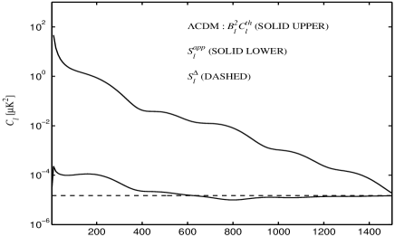
As shown in the bottom panel of Fig. 19 there is a good match between the analytical approximation of the signal bias $S_{\ell}^{app}$ and the signal bias estimate $S_{\ell}^{\mathrm{MC}}$ derived from the MC realizations.

One might have expected that increasing the map resolution (decreasing the pixel size) would have reduced the high-$\ell$ tail of the signal bias (and the filter function) or at least would have shifted it to higher multipoles. Contrary to this expectation the high-$\ell$ tail remains almost unaltered when the map resolution is increased (see Fig. 22). We can now explain this. The temperature differences $T_{ik}-T_{k}$ in average and the pixel size $\Omega_{p}$ become smaller when the pixel size is reduced. This would imply decreased $\Delta T_{k}$ and $S_{\ell}^{\Delta}$. However, when the pixel size is reduced there will be in average lower number of hits per pixel and those hits will be more unevenly spread inside the pixel area. An uneven spread would yield increased $\Delta T_{k}$. The net effect of these two opposite phenomena is that the magnitude of $S_{\ell}^{\Delta}$ remains nearly unaltered in this case and the high-$\ell$ tail remains roughly in the same place.

Figure 22: Same as the bottom panel of Fig. 19 but now the input map and output map had higher resolutions ($N_{\mathrm{side}}=2048$ and $N_{\mathrm{side}}=1024$, respectively).

In other words, the crucial resolution element here is not the pixel size, but the distance between neighboring detector pointings, separated by 3.3 arcmin along the ring, the rings themselves being separated by 2.5 arcmin.

A.2.2 Multiple Detectors

Destriping can be extended straightforwardly from a single detector TOD to multiple TODs produced by several detectors. The baselines can be determined jointly for all detectors and subtracted from the TODs. A single multidetector map can be obtained by considering the hits of all detectors in a pixel. The pseudo power spectrum can be extracted from the obtained multidetector map.

The signal bias will be altered when data from several detectors are combined, since that increases the density of detector pointings. To study this issue the pointing matrices of 70 GHz detectors of PLANCK LFI instrument were available. There are totally six LFI detectors at 70 GHz. Each single detector pointing matrix covered 12 months of observations. We calculated the analytical approximation $S_{\ell}^{app}$ of the signal bias by utilizing Eqs. (35), (36), (37), (39) and (40). The number of detectors was modelled by extending the calculations over the respective number of pointing matrices. It should be noted that due to differences in the sky coverage, in the mission time and in the sampling rates the absolute levels of the signal biases of LFI 70 GHz and 100 GHz detectors cannot be directly compared here. The results obtained with 70 GHz detectors reveal the relative impact that the number of detectors will have on the signal bias of the pseudo power spectrum extracted from a multidetector map.

The signal biases of one, three and six detectors are depicted in Fig. 23. At low $\ell$ ($\ell<300$) the signal bias is nearly independent of the number of detectors. The absolute level of the signal bias is highest at this range of multipoles. At high $\ell$ ($\ell>1200$) the signal bias is clearly dependent on the number of detectors. At this range of multipoles the signal bias is dominated by $S_{\ell}^{\Delta}$. The ratio between one detector and three detector $S_{\ell}^{\Delta}$ is 3.15. The respective ratio between one detector and six detector $S_{\ell}^{\Delta}$ is 5.83. Thus the high-$\ell$ level of $S_{\ell}^{app}$ is nearly inversely proportional to the number of detectors involved. At the medium range of $\ell$’s the behavior is more complex due to the abrupt change of sign of $S_{\ell}^{x\Delta}$.

Figure 23: Analytical approximations ($S_{\ell}^{app}$) of the signal biases of one (A), three (B) and six (C) combined detector signals. The bias of one detector is the mean of the signal biases of the individual 70 GHz LFI detectors. The bias of three detectors is obtained by considering the pointings of 70 GHz LFI detectors 18, 19 and 20. The pixel size of the output map was according to $N_{\mathrm{side}}=512$ and all the detector pointings fell in the centres of $N_{\mathrm{side}}=1024$ pixels. The horizontal lines show the contribution of $S_{\ell}^{\Delta}$ in each case. Dashed lines indicate negative values of $S_{\ell}^{app}$. The cosmological model was $\Lambda$CDM.

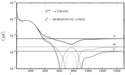
In light of this information, the level of the signal bias of a LFI 100 GHz detector can be compared to the typical level of the angular power spectrum of the instrument noise. The absolute level of the signal bias is highest at low $\ell$ and this part is nearly independent of the number of detectors involved. Comparing the analytical signal bias of Fig. 21 (single detector case) to the angular spectrum of the instrument noise (shown for the modelled full set of 24 detectors in the bottom panel of Fig. 1) one can notice that in this case the low-$\ell$ level of the noise bias is at least couple of orders of magnitude higher than the respective level of the signal bias.

A.3 Estimating the Signal Bias

In a real CMB experiment we will not have the true angular power spectrum $C_{\ell}^{th}$ available for estimating $S_{\ell}$. Since we have concluded that its dependence on $C_{\ell}^{th}$ is weak, this is not a concern. In place of $C_{\ell}^{th}$ we can use the noisy power spectrum estimate $\widehat{C}_{\ell}$ that is obtained from the real data.

In order to produce the noisy power spectrum estimate a single realization of the signal+noise pseudo power spectrum $\widetilde{C}_{\ell}$ was generated by following the procedure described in Section 6. A single 100 GHz LFI detector was considered. The estimate $\widehat{C}_{\ell}$ was solved from Eq. (15) by setting $S_{\ell}$ = 0 and by using $\langle\widetilde{N}_{\ell}\rangle$ determined according to the pure noise MC procedure (see Section 6). The obtained $\widehat{C}_{\ell}$ was binned with $\Delta\ell$ = 10 bins at $\ell\leq 1200$ and with $\Delta\ell$ = 50 bins at $\ell>1200$ and smoothed by a cubic spline (Fig. 10, top panel).

The noisy power spectrum estimate was used as the input spectrum for signal-only MC simulations ($N_{\rm MC}^{(\rm s)}=450$) to produce the estimate of the signal bias (Fig. 10, bottom panel). Destriping was applied in the map-making. As expected, the signal bias has a remarkable resemblance to the signal bias obtained from simulations with the true $\Lambda$CDM spectrum (see Fig. 19).

References

- Balbi et al. (2002) Balbi A., de Gasperis G., Natoli P., Vittorio N., 2002, A&A, 395, 417
- Bennett et al. (1996) Bennett C.L. et al., 1996, ApJ, 464, L1
- Bennett et al. (2003) Bennett C.L. et al., 2003, ApJS, 148, 1
- Bersanelli et al. (1996) Bersanelli M. et al., 1996, ESA, COBRAS/SAMBA Report on the Phase A Study, D/SCI(96)3
- Burigana et al. (1997) Burigana C., Malaspina M., Mandolesi, N., Danse L., Maino D., Bersanelli M., Maltoni M., 1997, Int. Rep. TeSRE/CNR, 198/1997 (astro-ph/9906360)
- Delabrouille (1998) Delabrouille J., 1998, A&AS, 127, 555
- Doré et al. (2001) Doré O., Teyssier R., Bouchet F.R., Vibert D., Prunet S., 2001, A&A,374, 358
- Efstathiou (2003) Efstathiou G., 2003, submitted to MNRAS, (astro-ph/0307515)
- Górski et al. (1996) Górski K.M., Banday A.J., Bennett C.L., Hinshaw G., Kogut A., Smoot G.F., Wright E.L., 1996, ApJ, 464, L11
- Górski, Hivon & Wandelt (1999) Górski K.M., Hivon E., Wandelt B.D., 1999, in Banday A.J., Sheth R.S., Da Costa L., eds, Proc. MPA/ESO Cosmology Conference ”Evolution of Large-Scale Structure”. PrintPartners Ipskamp, NL, p. 37. (astro-ph/9812350)
- Hivon et al. (2002) Hivon E., Górski K.M., Netterfield C.B., Crill B.P., Prunet S., Hansen F., 2002, ApJ, 567, 2
- Hobson & Magueijo (1996) Hobson M.P., Magueijo J., 1996, MNRAS, 283, 1133
- Janssen et al. (1996) Janssen M. et al., 1996, Report PSI-96-01, FIRE-96-01 (astro-ph/9602009)
- Keihänen et al. (2003) Keihänen E., Kurki-Suonio H., Poutanen T., Maino D., Burigana C., 2003, submitted to A&A (astro-ph/0304411)
- Knox (1995) Knox L., 1995, Phys. Rev. D 52, 4307
- Maino (1999) Maino D., 1999, PhD thesis, SISSA, Trieste, Italy
- Maino et al. (1999) Maino D. et al., 1999, A&AS, 140, 383
- Maino et al. (2002) Maino D., Burigana, Górski K.M., Mandolesi N., Bersanelli M., 2002, A&A, 387, 356
- Mennella et al. (2002) Mennella A., Bersanelli M., Burigana C., Maino D., Mandolesi N., Morgante G., Stanghellini G., 2002, A&A, 384, 736
- Natoli et al. (2001) Natoli P., de Gasperis G., Gheller C., Vittorio N., 2001, A&A, 372, 346
- Natoli et al. (2002) Natoli P., Marinucci D., Cabella P., de Gasperis G., Vittorio N., 2002, A&A, 383, 1100
- Netterfield et al. (2002) Netterfield C.B. et al., 2002, ApJ, 571, 604
- Oh, Spergel & Hinshaw (1999) Oh S.P., Spergel D.N., Hinshaw G., 1999, ApJ, 510, 551
- Scott, Srednicki & White (1994) Scott D., Srednicki M., White M., 1994, ApJ, 421, L5
- Seljak & Zaldarriaga (1996) Seljak U., Zaldarriaga M., 1996, ApJ, 469, 437
- Tauber (2000) Tauber J., 2000, in Harwitt M., Hauser M., eds, Proc. IAU Symp. 204, The extragalactic infrared background and its cosmological implications
- van Leeuwen et al. (2002) van Leeuwen F. et al., 2002, MNRAS, 331, 975
- Wandelt & Hansen (2003) Wandelt B.D., Hansen F.K., 2003, Phys. Rev. D 67, 023001