Fluid Stability Below the Neutrinospheres of Supernova Progenitors and the Dominant Role of Lepto-Entropy Fingers
Abstract
Instabilities driven by thermal and lepton diffusion (doubly diffusive instabilities) in a Ledoux stable fluid will, if present below the neutrinosphere of the collapsed core of a supernova progenitor (proto-supernova), induce convective-like fluid motions there. These fluid motions may enhance the neutrino emission by advecting neutrinos outward toward the neutrinosphere, and may thus play an important role in the supernova mechanism. “Neutron fingers,” in particular, have been suggested as being critical for producing explosions in the sophisticated spherically symmetric supernova simulations by the Livermore group (Wilson & Mayle, 1993, e.g.,). These have been argued to arise in an extensive region below the neutrinosphere of a proto-supernova where entropy and lepton gradients are stabilizing and destabilizing, respectively, if, as they assert, the rate of neutrino-mediated thermal equilibration greatly exceeds that of neutrino-mediated lepton equilibration. Application of the Livermore group’s criteria to models derived from core collapse simulations using both their equation of state and the Lattimer-Swesty equation of state do indeed show a large region below the neutrinosphere unstable to neutron fingers.
Because of the potential importance of fluid instabilities for the supernova mechanism, and the desire to understand the origin of convective-like fluid motions that may arise in upcoming multi-dimensional radiation-hydrodynamical simulations of core collapse, we develop a methodology introduced by Bruenn & Dineva (1996) for analyzing the stability of a fluid in the presence of neutrinos of all flavors and in the presence of a gravitational field. Neutrino-mediated thermal and lepton equilibration between a fluid element and its surroundings (background) is modeled as a linear system characterized by four response functions (i.e., thermal and lepton equilibration driven by entropy and lepton fraction differences between a fluid element and the background), the latter evaluated for a given thermodynamic state and fluid element radius by detailed neutrino transport simulations. These transport simulations employ both traditional and improved neutrino physics.
When applied to an extensive two-dimensional grid of core radii and fluid element sizes for each of several time slices of a number of proto-supernovae, we find no evidence for the neutron finger instability as described by the Livermore group. We find, instead, that the rate of lepton equilibration always exceeds that of thermal equilibration. Furthermore, we find that neither of the “cross” response functions, that is, entropy equilibration driven by a lepton fraction difference, and lepton equilibration driven by an entropy difference, is zero and that the first of these tends to be the largest of the four response functions in magnitude. These cross response functions play a critical role in the dynamics of the equilibration of a fluid element with the background. An important consequence of this is the presence of a doubly diffusive instability, which we refer to as “lepto-entropy fingers,” in an extensive region below the neutrinosphere where the lepton number, , is small. This instability is driven by a mechanism very different from that giving rise to neutron fingers, and may play an important role in enhancing the neutrino emission. Deep in the core where the entropy is low and the lepton number higher, our analysis indicates a region unstable to another instability, also involving the cross response functions, which we refer to as “lepto-entropy semiconvection.” These instabilities, particularly lepto-entropy fingers, may have already been seen in some multi-dimensional core collapse simulations described in the literature.
Subject headings:
(stars:) supernovae: general – neutrinos – fluid instabilities1. Introduction
It has long been recognized that fluid instabilities may play an important role in the supernova mechanism. It is generally agreed that entropy driven convection between the neutrinosphere and the shock during the postbounce phase of the collapsed core of a supernova progenitor (hereafter ”proto-supernova”) will contribute turbulent pressure and increase the neutrino energy-deposition efficiency (Bethe, 1990; Miller et al., 1993; Herant et al., 1994; Burrows et al., 1995; Janka & Müller, 1996; Mezzacappa et al., 1998b; Fryer, 1999; Fryer & Warren, 2002; Buras et al., 2003), but this may not be enough to produce explosions.
More controversial is the nature and the role of fluid instabilities below the neutrinosphere. Here matter and neutrinos are tightly coupled, and convective-like motions induced by instabilities can advect neutrinos. If these convective-like motions occur between the deeper interior and the neutrinosphere, ’s could be advected from the lepton rich deeper interior to the neutrinosphere, thus adding to the rate of diffusion and enhancing the luminosity. The analysis of fluid instabilities below the neutrinosphere must take into account the possibilities of thermal and lepton transfer by neutrinos. For example, a displaced fluid element in the presence of an entropy and/or lepton fraction gradient will find that its entropy and/or lepton fraction will differ from that of its surroundings or background. This will induce neutrino mediated thermal and lepton transfer which can modify the hydrodynamic buoyancy forces felt by the fluid element. This in turn can modify the subsequent growth rate of an instability, or the very existence of an instability. In particular, instabilities can arise in a gravitating fluid because of thermal and lepton transport that would otherwise be stable in their absence. These instabilities, involving the transport of two quantities (e.g., energy and leptons), are referred to as doubly diffusive instabilities.
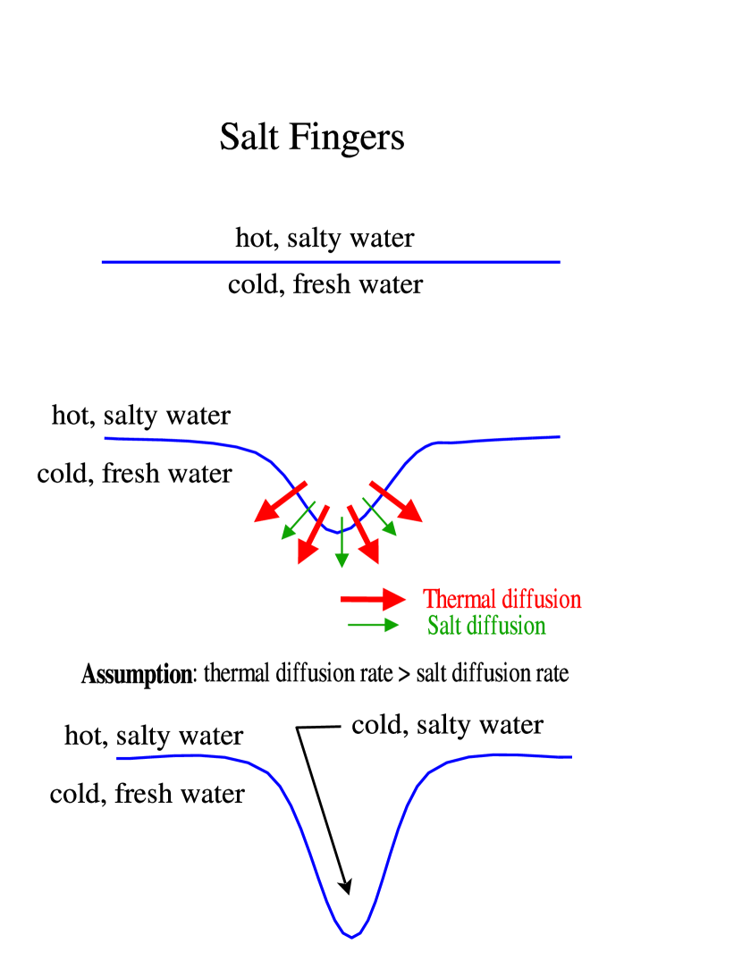
To introduce the phenomenon, let us consider several classic examples of doubly diffusive instabilities. A doubly diffusive instability will arise if there are two differing “substances,” say heat and leptons, with gradients that can act oppositely in their stabilizing effects. For the sake of a concrete model, consider the case of heat and salt in water. Let us first imagine the case in which a region of hot salty water overlies a region of cold fresh water (Stern, 1960). Normally the diffusion of heat occurs more rapidly than the diffusion of salt, and we will assume this to be the case here. Let us also assume that the magnitudes of the gradients in heat and salt are such that the fluid is stably stratified gravitationally (i.e., Ledoux stable). Imagine a parcel of hot salty water to be depressed slightly, as shown in Figure 1. The rapid diffusion of heat will thermally equilibrate this parcel of water with the background, but the slower diffusion of salt will result in the water remaining salty. We thus end up with a pocket of cold salty water in a background cold fresh water, and this pocket, being denser than the background, will continue to sink. The result is that “fingers” of salty water will poenetrate the fresh water on a thermal diffusion time scale. Note that what creates the instability in this otherwise stable situation is the presence of diffusion, and thus its description as a “diffusive instability.” The above described instability is referred to as salt fingers, and is an example of the kind of doubly diffusive instability that occurs if a slowly diffusing substance with a destabilizing gradient is stabilized in the absence of diffusion by the gradient of a rapidly diffusing substance.
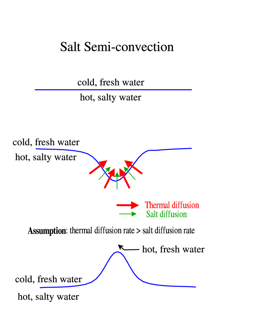
Now imagine that the spatial configuration described above is reversed, namely, that a region of cold fresh water overlies a region of hot salty water, so that the gradient of salt is now stabilizing, the gradient of heat dstabilizing, and the magnitudes of the gradients such that the fluid is Ledoux stable (Veronis, 1965). Imagine further that a parcel of cold fresh water is depressed slightly into the hot salty water, as shown in Figure 2. Again the rapid diffusion of heat will thermally equilibrate the parcel with the background, but the slower diffusion of salt will result in the parcel remaining fresh. We thus end up with a parcel of hot fresh water in a background of hot salty water, and the parcel, being less dense than originally from the background, will accelerate upwards faster than would have been the case with no diffusion. This can result in an overstable situation, driven by the phase lag between the temperature and velocities of the fluid element which causes net work to be done over each cycle (Spiegel, 1972). In this case the parcel will oscillate with growing amplitude. This instability is referred to as “semiconvection,” and is an example of the kind of doubly diffusive instability that occurs if a rapidly diffusing substance with a destabilizing gradient is stabilized in the absence of diffusion by a slowly diffusing substance with a stabilizing gradient.
Doubly diffusive instabilities such as described above can occur in the collapsed core of a supernova progenitor (Smarr et al., 1981). Neutron rich (low , where is the proton fraction) matter tends to be denser than neutron poor (high ) matter at the same temperature and pressure because the latter contains more light particles (electrons and electron neutrinos) that contribute to the pressure. Thus neutron richness in stellar cores can be thought of as playing a role analogous to that of salt in the discussion above. The ramp-up of the bounce shock on core rebound results in an outwardly positive (stabilizing) entropy gradient throughout much of the inner core. On the other hand, a negative lepton gradient formed at and initially confined to the vicinity of the -sphere immediately after shock breakout is advected deeper into the core with time because of the inward matter flow and outward diffusion of ’s. A destabilizing negative gradient stabilized by the outwardly positive entropy gradient can set the stage for a doubly diffusive instability analogous to salt fingers if lepton transport is slower than thermal transport. This instability is referred to as “neutron fingers.”
The Livermore group has reported successful explosions in their spherically symmetric supernova simulations employing sophisticated multi-energy neutrino transport, and have emphasized the importance of the neutron-finger instability in powering these explosions (Wilson et al., 1986; Wilson & Mayle, 1988, 1993). The issue of whether or not this instability is operative, and if so whether or not it will power an explosion is important, as no other supernova simulations employing neutrino transport of comparable sophistication but without invoking neutron fingers has produced an explosion (Bruenn, 1993; Mezzacappa et al., 2001; Liebendörfer et al., 2001; Buras et al., 2003).
The Livermore group argue that thermal equilibration between a fluid element and the background is driven by the total neutrino number density (i.e., ’s, ’s, and ’s and their antiparticles), whereas equilibration in composition (i.e., lepton fraction, ) is driven only by the difference in the number densities of ’s and ’s. The ratio, , of the two equilibration rates is thus given approximately by
| (1) |
where is the number density of neutrinos of type . From their simulations they typically find that . Based on the magnitude of this inequality the Livermore group tests for the neutron-finger instability by displacing a fluid element at constant composition but equilibrated with the background material in pressure and temperature. If the density of the fluid element relative to its surroundings after displacement is such as to drive the displacement further, the fluid is taken to be neutron-finger unstable. Mathematically, their criterion for neutron-finger instability is given by
| (2) |
where is the gradient of the background. If a region was established to be neutron-finger unstable, a mixing length algorithm was then employed to simulate the convective fluid motions and mixing. The Livermore group found that the result of the convective-like motions due to the neutron-finger instability in their supernova simulations was the production of a larger luminosity, as neutrinos and electrons previously trapped in the core were brought to the vicinity of the neutrinosphere. This increase in luminosity was found to be sufficient to power an explosion.
In several papers, Bruenn et al. (1995) and Bruenn & Dineva (1996) questioned the assumption that the ratio, , of the rates of composition to thermal equilibration is given by equation (1). Situations were envisioned in which a fluid element perturbed with respect to the background could drive counter flows of ’s and ’s so that the numerator of equation (1) would be additive in and and the denominator subtractive. Detailed simulations, performed by Bruenn & Dineva (1996), of the equilibration of fluid elements perturbed with respect to the background showed that in many cases counter flows of ’s and ’s did indeed occur. Furthermore, it was found that lepton transport proceeded quickly by the rapid transport of low energy ’s and ’s, as the opacity for these was relatively small. On the other hand, thermal equilibration, being more efficiently accomplished by high energy neutrinos, was slowed by the relatively large opacities encountered by these neutrinos. Finally, the ’s, ’s, and their antiparticles were less effective at mediating thermal equilibration because of there weak thermal coupling with the matter. The result was that the ratio of composition to thermal equilibration depended on how the fluid element was perturbed with respect to the background, and in many cases this ratio was greater than unity.
Given its potential role in the core collapse supernova mechanism, there is clearly a need to clarify the issue of the neutron-finger instability in a proto-supernova. Additionally there has been the advent during the past decade of multi-dimensional core collapse supernova modeling (Miller et al., 1993; Herant et al., 1994; Burrows et al., 1995; Janka & Müller, 1996; Mezzacappa et al., 1998a, b; Fryer, 1999; Fryer & Warren, 2002; Buras et al., 2003), with more simulations of greater sophistication to come. The extant simulations show the presence of fluid instabilities both above and below the neutrinosphere. The fluid instabilities above the neutrinosphere are driven by neutrino heating immediately above the gain radius, which is the surface above the neutrinosphere where neutrino cooling and heating balance. This instability is analogous to that of a fluid in a pot heated from below. The fluid instabilities below the neutrinosphere are more complicated to characterize, as neutrino transport drives both thermal and composition changes and the fluid instabilities can be doubly diffusive.
Bruenn & Dineva (1996) developed a procedure for characterizing the stability/instability of a fluid element as a function of the entropy and composition gradient of the background and found that for typical conditions inside the collapsed stellar core of a supernova progenitor the fluid was either unstable to semiconvection or stable. However, they sampled only a small region of the run of thermodynamic conditions inside a supernova progenitor. In this paper we will further develop the methodology of Bruenn & Dineva (1996) and use it to examine the stability of proto-supernovae for the entire run of thermodynamic conditions from the center of the core to the neutrinosphere. Futhermore, for each set of thermodynamic conditions we will consider the stability as a function of the size of the fluid element. The latter is important in that it governs the rate of thermal and composition equilibration. In Section 2 we begin our discussion of fluid stability in the ambience of neutrino mediated thermal and lepton transport by presenting the equations of motion of a fluid element that we will use to analyze stability. These equations involve four response functions that describe how thermal and lepton diffusion is driven by an entropy or a lepton fraction difference between a fluid element and the background. In Section 3 we describe how the solutions of these equations of motion are used to define various types of instability. We also examine the stability of a fluid element as a function of the entropy and lepton gradients of the background for various representative sets of the “response functions.” These examples illustrate the different kinds of instabilities that can arise in a proto-supernova. In particular, we find that neutron fingers is unlikely to occur anywhere below the neutrinosphere. However, we discover and describe several new and potentially important modes of doubly diffusive instabilities which we refer to as “lepto-entropy fingers” and “lepto-entropy semiconvection.” Both of the instabilities involve the cross response functions in essential ways. In Section 4 we describe how the response functions are computed for a given thermodynamic state and fluid element size. In Section 5 we begin the application of our stability analysis to core collapse models by describing these models, and in Section 6 we present the results of an extensive set of calculations giving the stability or type of instability and its growth rate as a function both the fluid element size and its location in the core. In Section 7 we compare our analyses and results with prior work, and in in Section 8 we present our conclusions.
2. Single Particle Analysis
We consider a mix of hot, dense material and neutrinos at conditions typical of the region below the neutrinosphere of a proro-supernova ( g cm-3, MeV, . Such a mix can be considered to be equilibrated with respect to strong, electromagnetic, and weak interactions. Its thermodynamic and compositional states can therefore be specified by three independent variables, which we take to be the pressure , entropy , and lepton fraction fraction .
In a manner analogous to Grossman et al. (1993), we consider the behavior of an individual fluid element in a background which is assumed to be time-independent and one-dimensional. The z-axis is taken normal to the plane of symmetry and the background is assumed to have constant gradients in entropy and lepton fraction . We will assume that the fluid element is always in pressure equilibrium with the background, i.e., , where unmarked and barred variables refer to the fluid element and the background, respectively. However, the fluid element and the background may differ locally in and , and these differences will be denoted by the quantities and , where and . Given , , and , the thermodynamic state of the fluid element is given by its values of , , and its vertical location (positive for directions away from the center of the core) through
| (3) |
| (4) |
| (5) |
The quantities , and , will change with time by the effect of energy and lepton transport by neutrinos, and by the vertical motion of the fluid element through the gradients of and of the background. We assume that neutrino energy and lepton transport is linear for small , and and describe it by the four “response functions” , , , and , defined by
| (6) |
Thus, gives the rate of change of due to the presence of a nonzero entropy difference, , and a zero lepton fraction difference, , between the fluid element and the background, gives the rate of change of due to the presence of a nonzero lepton fraction difference, , and a zero entropy difference, , and so forth. With these definitions, it follows that
| (7) |
and
| (8) |
where and are the rate of change respectively of and due to neutrino transport. The presence of the “cross” response functions and is due to the fact that, (1) entropy transport is brought about by both thermal and lepton transport, (2) that neutrinos transport both energy and leptons, and (3) that transport is inherently a dissipative process. Thus, for example, a difference, , in can force a rate of change of as well as , as can a difference, , in . These cross response functions introduce important additional patterns of stability/instability behavior as a function of the gradients in and , as will be described below. Discussions of doubly diffusive instabilities apart from the proto-supernova problem and prior to Bruenn & Dineva (1996) did not relate to a context in which cross response functions were important, and these were not considered.
The equations for and are completed by adding to equations (7) and (8) the effect of the vertical motion of the fluid element, , to get
| (9) |
| (10) |
The equation of motion for the fluid element is given by the buoyancy acceleration driven by the difference between its density and that of the background, viz.,
| (11) |
where is the magnitude of the acceleration of gravity.
3. Stability Analysis
To investigate the stability of a fluid element described by equations (9) - (11), we regard these equations as giving the time evolution of , , and and consider in this Section classes of possible time dependent behaviors of a fluid element perturbed from equilibrium as a function of the gradients in and , the radius, , of the fluid element, and the gravitational force, . In particular, we look for solutions of the form
| (12) |
where the eigenvalues, , will determine the stability of the fluid, as described below.
In Sections 3.1 - 3.3 we look at some particular cases where the response functions take on simplified and special sets of values. The purpose is to relate some classic examples of instability to the solutions of equations equations (9) - (11), and to build from the simple to the complex. We delay until Section 3.4 an analysis of the general case in which all four response functions have arbitrary nonzero values. The reader who is interested in proceeding directly the the general case is advised to skip directly to Section 3.4.
3.1. Ledoux Stability Limit
We begin with a well-known case by considering the limit in which there is no thermal or lepton transport (i.e., the limit in which all four response functions are zero). Instability in this case is referred to as Ledoux instability, and equations (9) - (11) in this case reduce to
| (13) |
| (14) |
| (15) |
The eigenvalues are given by
| (16) |
with the solutions
| (17) |
where we define and by
| (18) |
Physically, if then is the frequency that a fluid element would oscillate about a stable equilibrium if , and the growth rate that would characterize the motion of a fluid element away from an unstable equilibrium if . has an analogous interpretation, e.g., if then is the frequency that a fluid element would oscillate about a stable equilibrium if , and the growth rate that would characterize the motion of a fluid element away from an unstable equilibrium if . and thus characterize the effect of the background gradients, and , respectively, on the dynamics of a fluid element perturbed from equilibrium. In equation (17), the solution arises from the fact that a fluid element at rest and having the same thermodynamic conditions as the background (i.e., ) will remain at rest. Note, however, that the equilibrium implied by the solution may not be a stable equilibrium.
The criterion for Ledoux stability is that the eigenvalues be imaginary, which requires the following inequality be satisfied:
| (19) |
If this inequality is satisfied, then the two solutions, , can be written
| (20) |
where
| (21) |
is the Brunt-Väisälä frequency. In this case the fluid element will oscillate about the equilibrium configuration with the angular frequency and constant amplitude. This situation is therefore stable. On the other hand, if inequality (19) is not satisfied, i.e., if
| (22) |
then the solutions, and , can be written , with the positive solution corresponding to an exponentially growing amplitude with growth rate given by
| (23) |
In this case the fluid is said to be convectively unstable. Thus, in the case of no thermal or lepton transport, the “Ledoux critical line”
| (24) |
separates, in the - plane, a convectively stable region where the left-hand side of equation (24) is from a convectively unstable region where the left-hand side of equation (24) is .
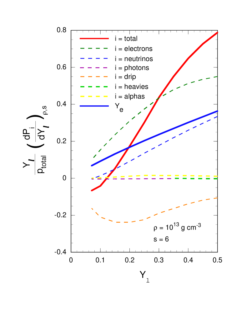
It is interesting to consider the signs of the coefficients of and in equation (24). The derivative is equal to , where is the always positive constant pressure specific heat and is the expansivity. Provided the latter is positive, which is almost always the case, the derivative is negative, and a positive gradient is is therefore stabilizing. On the other hand, the derivative is equal to , where is the isentropic compressibility (always positive), so the sign of can be negative or positive depending on the sign of . The latter can be positive or negative depending on the magnitude of . To explain this curious behavior, note that increasing increases the number of light particles while leaving the baryon number essentially unchanged. The entropy, which is being held constant in , depends on both the number of particles and the temperature. Increasing the former will typically (but not always) require a decrease in the latter in order to maintain constant entropy, and the pressure can therefore increase or decrease. Whether increases or decreases depends on which particle specie is dominating the pressure. Figure 3 shows the contribution of the various particle species to . It is seen that the light particles (e-’s and ’s) provide a positive contribution to for all values of for the given thermodynamic conditions, due to their partial degeneracy, but the baryons are nondegenerate and provide a negative contribution. For values of above 0.11, and for the indicated values of and , the contribution of e-’s and ’s to dominate and this derivative is positive. But for values of below 0.11 the baryons dominate and this derivative is negative. For values of close to 0.11 this derivative, and therefore , is almost zero. The stability of a fluid element in this latter regime is extremely insensitive to the gradient , and the Ledoux critical line is almost vertical.
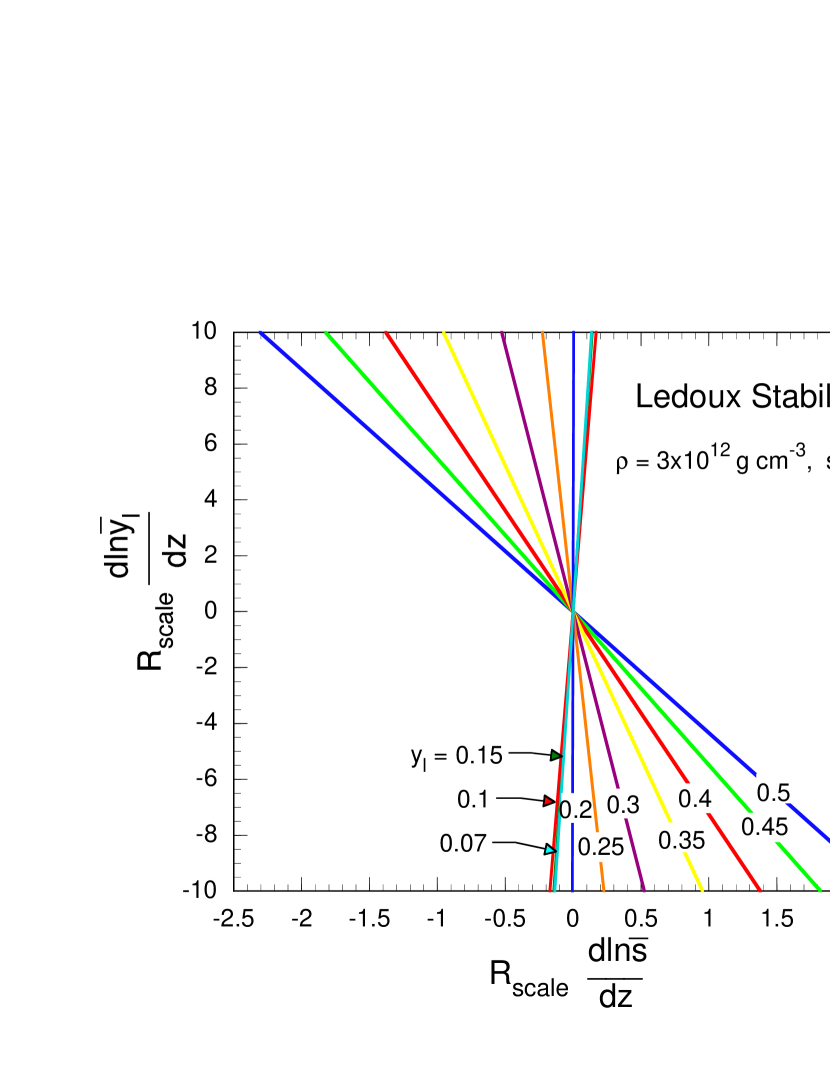
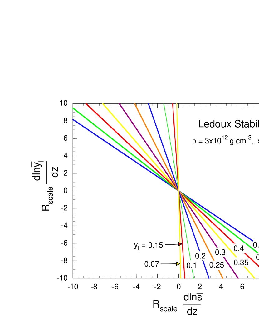
To exemplify the above discussion, Figure 4 shows the Ledoux critical line as a function of for the indicated values of and . As decreases it is seen that the slope of the Ledoux critical line goes from negative through the vertical to positive. The meaning of a positive slope for the critical line is that a negative (destabilizing) gradient in is now balanced by a negative rather than a positive gradient in . At lower entropies, on the other hand, such as the case of shown in Figure 5, the baryons do not dominate the derivative even for as low as 0.07, and the slope of the Ledoux critical line remains negative for all values of shown.
The sign change in the slope of the Ledoux critical line as falls below a critical value will have important ramifications below for the locations of the instability regions in the - plane when we consider more general sets of values for the response functions.
3.2. Schwarzschild Stability Limit
Referring to and and to and as the direct and cross response functions, respectively, let us consider the case in which the former are nonzero while the latter are still zero. (That is, we take , , , and .) This corresponds to the case in which an entropy gradient drives an entropy, but not a lepton flow, and a lepton gradient drives a lepton but not an entropy flow. Then equations (9) - (11) become
| (25) |
| (26) |
| (27) |
Let us further suppose in this Section that , that is, that the fluid element is instantaneously equilibrated in with the background, leaving for the next Section the case in which is finite. If , it follows that which implies that , so equation (26) must reduce to
| (28) |
i.e., and such that . The equations for the nonzero variables now simplify to
| (29) |
| (30) |
Using the first and the last of equations (12), the condition for nontrivial solutions is
| (31) |
Let us consider the case and separately. If , then
| (32) |
where in the last expression we have explicitly taken into account the fact that . Equation (32) expresses the Schwarzschild stability criterion, viz., if then the roots are imaginary and the fluid is oscillatory stable, the oscillation frequency being defined in equation (18); if then there is one positive and one negative real root and the fluid is convectively unstable with a growth rate, , given by the magnitude of the positive root, e.g.,
| (33) |
The critical stability line, i.e., the line in the - plane that separates real from imaginary roots (instability from stability) is the vertical line .
Assume now that is as above (viz., ) but , and that , i.e., that neutrino transport will drive an entropy perturbation of a fluid element back towards equilibrium with the background. In this case the solutions of equations (25 - (27) are
| (34) |
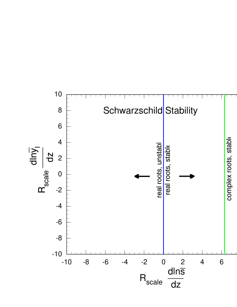
In contrast to the case in which and for which the critical stability line separates both the real and imaginary solutions and the unstable and stable regimes, with the critical line bifurcates into two parallel critical lines. The situation is shown schematically in Figure 6. The critical line , which we will refer to as critical line 1, is the line along which one real root is zero, and so changes sign as this line is crossed. It still separates stable from unstable solutions. However a second critical line now appears, which we refer to as critical line 2. Along this line two real roots switch to a complex conjugate pair, so this critical line separates real from complex solutions. To the right of the critical line 2 the fluid is stable; if perturbed it will oscillate with decreasing amplitude. Along critical 2 line the neutrino transport critically damps the fluid. In the region between the two critical lines the fluid is stable but non-oscillatory—neutrino transport overdamps the fluid. To the left () of the critical line 1 the fluid is unstable, as in the case, and equation (34) can be written
| (35) |
Close but to the left of critical line 1 separating stable from unstable solutions, where , or equivalently where , the growth rate, , of the instability is
| (36) |
The growth rate is thus reduced from the case by a factor of . This factor arises from the reduction in (and thus in the buoyancy force) due to the tendency of neutrino transport (as modeled by a negative ) to thermally equilibrate the fluid element with the background. Finally, far to the left of the first critical line, where , or equivalently where , the growth rate of the instability is
| (37) |
i.e., just slightly less than the case. Here there is also a reduction in (and thus in the buoyancy force) due to the tendency of neutrino transport to thermally equilibrate the fluid element with the background, but this effect is now small compared with the growth rate, , the fluid element would experience in the absence of transport.
Now imagine for a the moment that , i.e., that neutrino transport will drive an entropy perturbation of a fluid element further away from equilibrium. Then
| (38) |
In this case there is no stability. Critical line 1 () separates the region to its left where equation (38) gives one positive and one negative root from the region to the right but to the left of critical line 2 () where equation (38) gives two positive roots. To the right of critical line 2 equation (38) gives complex solutions with a positive real part — the motion of a perturbed fluid element in this case is oscillatory with a growing amplitude, i.e., semiconvective.
3.3.
We generalize the case considered in the preceding Section by allowing to be finite rather than - ; that is we consider the case in which the two “direct” response functions, and , are nonzero and arbitrary, but the two “cross” response functions, and , are still zero. Then equations (9) - (11) become equations (25) - (27), which are written here again as
| (39) |
| (40) |
and
| (41) |
Solutions have the form given by equations (12), and exist for values of satisfying
| (42) |
where
| (43) |
| (44) |
and
| (45) |
The eigenvalues, , in this case are given by the solution of a cubic equation, and so display a richer variety. In particular, there are now three roots rather than two. The three roots are either all real, or consist of one real root and a complex conjugate pair. In the above discussion of Schwarzschild stability, critical line 1 in the plane was defined as the line along which a root is zero, so that a root changes sign as this line is crossed (i.e., a stable/unstable mode switches to a unstable/stable mode). The analog of that line here is obtained by setting in equation (45) to zero. This gives
| (46) |
which we will also refer to as critical line 1. As in the above case of Schwarzschild stability, critical line 1 here is the line across which a root changes sign.
The second critical line in the plane introduced in our discussion of Schwarzschild stability was the line across which a pair of real roots switch to a complex conjugate pair (growing/decaying modes switch to growing/decaying oscillatory modes). The analog here is the line across which two real roots switch to a complex conjugate pair, and is obtained from the equation (Abramowitz & Stegun, 1965)
| (47) |
where
| (48) |
Thus, critical line 2 is given by equations (43) - (45), (47) and (48). This is a fairly messy nonlinear equation in and and will not be written down here. It will be solved numerically for a number of illustrative examples below.
Finally, and unlike the case of Schwarzschild stability, there is the possibility that the real part of a complex conjugate pair of roots can change sign. This will happen if there is a complex conjugate pair of roots, and if they sum to zero. To determine the condition for this note (Abramowitz & Stegun, 1965) that the roots of cubic equation (42) satisfy
| (49) |
Then gives
| (50) |
where the subscripts 1, 2, and 3 can be cyclically permuted in the above expressions. Thus equation (50) is satisfied if any two roots sum to zero. This is the desired condition. Using equations (43) - (45) equation can be written
| (51) |
and we will refer to this line as critical line 3.
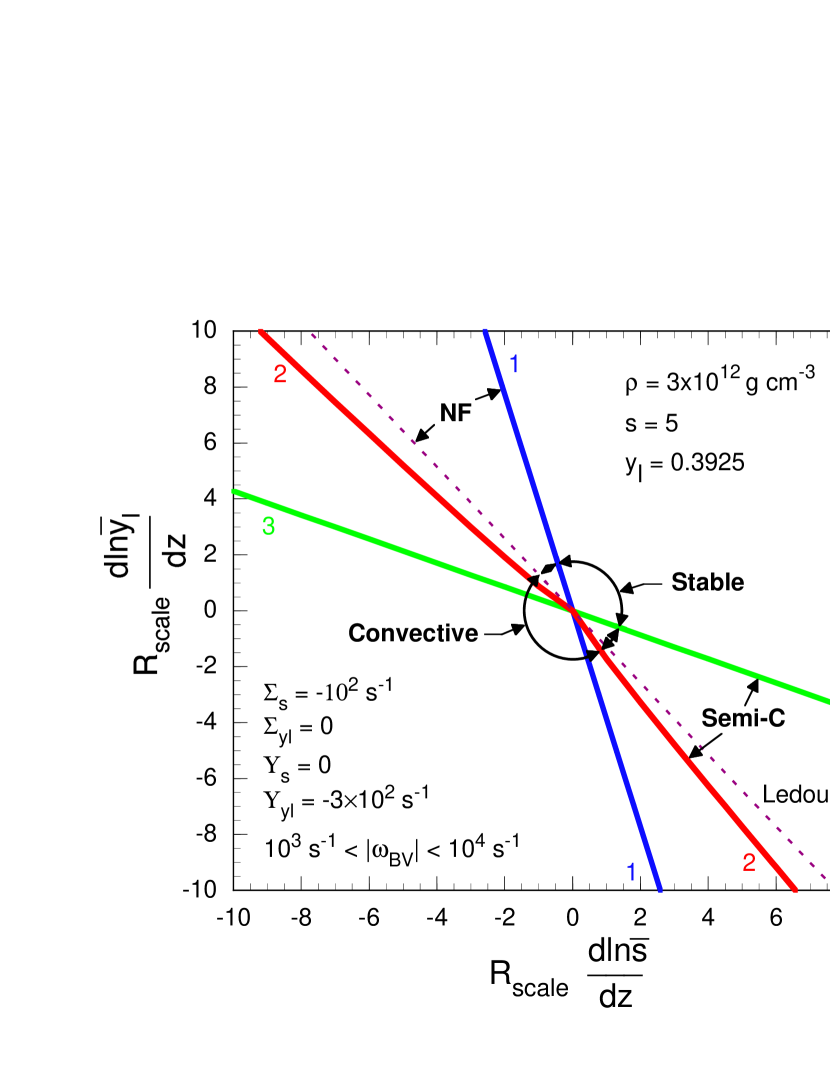
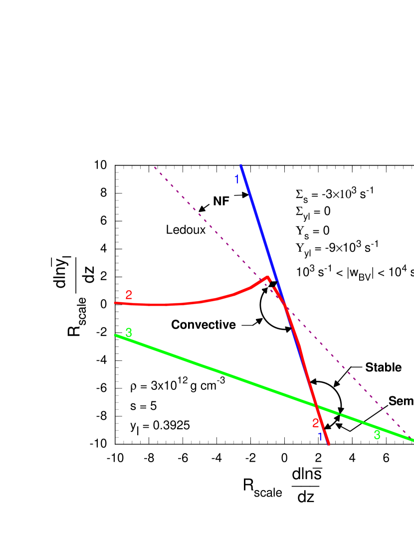
Figures 7 and 8 show these three critical lines along with the Ledoux line in the plane for the indicated thermodynamic state and values of , , and . The absolute value of the Brunt-Väisälä frequency, , where is given by equation (21), is an indicator of the buoyancy growth rate in the absence of neutrino transport. Its value, however, depends on the gradients of and and therefore varies over the plane. A range of typical values for is given in the figures. A comparison of these values with the absolute values, and , of the direct response functions will indicate the relative importance of buoyancy versus neutrino transport on the dynamics of the fluid element.
We have divided the plane into four distinct regions delimiting different types of fluid stability/instability, the boundary between any two adjacent regions being one of the critical lines. In the region denoted “stable” all roots of equation (42) are negative, if real, or have a negative real part if a complex conjugate pair. A perturbed fluid element in this region will return to its unperturbed state, and the fluid is therefore stable. In the region marked “Semi-C” the largest growth rate arises from the positive real part of a complex conjugate pair of roots, and the dominate unstable mode is therefore oscillatory and growing. In this region the fluid is unstable to semiconvection. In the region marked “NF” the largest growth rate arises from a positive real root, but the region resides on the stable side of the Ledoux critical line and would therefore be stable in the absence of thermal and lepton transport. The instability in this region is therefore driven by thermal and lepton transport. We refer to this instability for the moment as “neutron fingers,” although we will show below that for the conditions in the collapsed stellar cores of supernova progenitors that we have analyzed this instability is not neutron fingers per se but something quite different. Finally, in the region marked “convection” the largest growth rate arises from a positive real root, as in the NF case, but the region resides on the unstable side of the Ledoux critical line and would therefore be unstable even in the absence of thermal and lepton diffusion. We summarize our stability/instability classification in Table 1.
| Classification | Roots | Subsidiary Conditions |
|---|---|---|
| Stable | ||
| Semi-C | ||
| NF | Ledoux stable in the absence of transport | |
| Convection | Ledoux unstable in the absence of transport |
is the largest real root, or the real part of a complex conjugate pair. is the imaginary part of the root of which is the real part.
To characterize in more detail the stability/instability of the fluid in the plane for the conditions shown in Figure 7, and to delineate the role of the critical stability lines, we will start in the upper right quadrant of that figure where the gradients of and are both positive. The condition that the fluid is stable, i.e., that all the roots of equation (42) are negative, if real, or that the real root is negative and the real part of a complex conjugate pair is also negative, is that all of the following inequalities be fulfilled (Aleksandrov et al., 1963): , , and , where , , and are given by equations (43) - (45). , given by equation (43), is clearly positive, as both and are negative. For the given thermodynamic conditions the logarithmic derivatives and are both negative, therefore , given by equation (45), is also positive. Finally,
| (52) |
since each term to the left of the inequality sign of equation (52) is positive. Thus all three of the above inequalities are satisfied in the upper right quadrant of Figure 7 where the gradients of and are both positive, and the fluid is therefore stable in this region. For the particular case shown in Figure 7, in the upper right-hand quadrant there is a negative real root and a complex conjugate pair with a negative real part.
To characterize the stability/instability of the fluid in the remaining parts of the plane, let us move clockwise around the figure from the upper right-hand quadrant. The character of the roots (and therefore the stability of the fluid) does not change until critical line 3 is crossed, at which point the real part of the complex conjugate pair of roots changes sign from negative to positive. The fluid, if perturbed, will now oscillate with growing amplitude, and according to our taxonomy is therefore unstable to semiconvection. Continuing clockwise, critical line 2 is crossed and the complex conjugate pair of roots with positive real part become two real positive roots. The fluid, if perturbed, will move away from equilibrium with exponentially increasing amplitude. The fluid is therefore unstable in this region, and since it is would be Ledoux unstable in the absence of transport, it is therefore convective. Crossing line 1 at the bottom of the figure, one of the positive real roots changes sign, so there are now one positive real root and two negative real roots. Because of the positive real root the fluid is again convective. Continuing clockwise to the left of the figure and up, critical line 3 is crossed and the real part of a complex conjugate pair of roots, if present, would change sign. There not being a complex conjugate pair of roots in this region, there is no change in the character of the roots and the fluid remains convective. Continuing clockwise and crossing critical line 2 at the upper left-hand side of the figure, two negative real roots change to a complex conjugate pair with a negative real part, leaving one real positive root. The fluid is still convective. On crossing the Ledoux line the character of the roots remains unchanged but the fluid would be stable in the absence of thermal and lepton transport. The fluid is now unstable to neutron fingers. Finally, crossing critical line 1 from left to right at the top of the figure the positive real root changes sign and we are left with a negative real root and a complex conjugate pair with a negative real part. We are back in the region where the fluid is stable.
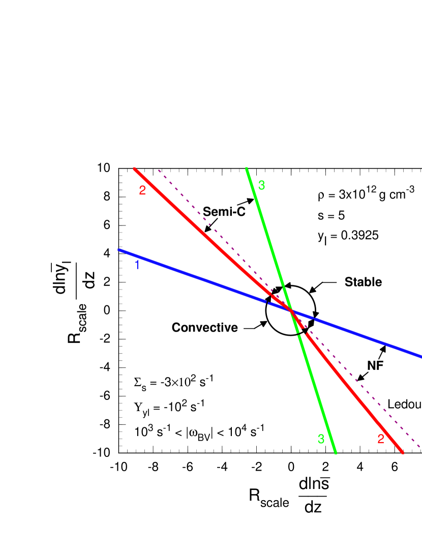
The above taxonomical sectoring of the plane in Figure 7 into regions of stability, convection, semiconvection, and neutrino fingers is a general characterization of a gravitating fluid with thermal and lepton transport represented by negative values for and . The location of these regions will depend, however, on the magnitudes of and , and on the thermodynamic state of the fluid and the force of gravity. Figure 7 has illustrated a case in which (lepton equilibration more rapid than thermal equilibration). Interchanging the values of and , so that (thermal equilibration more rapid than lepton equilibration), and keeping the same thermodynamic state and gravity gives regions of stability and instability shown in Figure 8. Note, as is apparent from equations (46) and (51), that interchanging the values of and interchanges the slopes of critical lines 1 and 3 (and also changes the intercept of critical line 3). Also, the location of the NF and Semi-C regions are interchanged. Referring back to the discussion in Section 1, Figures 7 and 8 show, respectively, that a destabilizing (negative) gradient in stabilized by a stable (positive) gradient in leads to semiconvection if (lepton transport more rapid than thermal transport) and neutron fingers if (thermal transport more rapid than lepton transport). The opposite is true if the destabilizing (negative) gradient is and the stabilizing (positive) gradient is (tops of Figures (7) and (8).

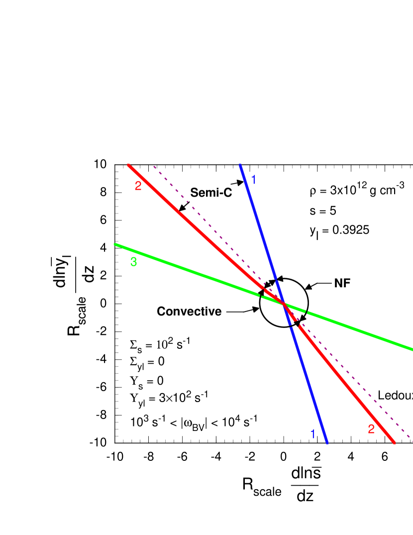
Figures 9 and 10 show the effect of successively increasing the values of and , but keeping their ratio the same, and keeping the thermodynamic state and gravitational acceleration the same (all equal to the case shown in Figure 7). It is apparent from equations (46) and (51) that the slopes of critical lines 1 and 3 are unaffected by the magnitudes of and provided that their ratio remains the same. However, the intercept of critical line 3 with the vertical axis becomes more negative (recall that is negative for the case being considered). The latter effect is to extend the stable region with increasing magnitudes of and into the region that was formerly semiconvective.
An effect not evident from the figures is the dependence of the instability growth rates on the magnitudes of and for given values of the gradients and . Qualitativelly, the growth rates for instabilities that are driven by thermal or lepton transport (semiconvection or neutron fingers) increase with the magnitudes of and , while those that are buoyancy driven (convection) decrease with the magnitudes of and . The latter effect arises because thermal and lepton transport tend to equilibrate the perturbed fluid element with its surroundings, thus reducing the buoyancy forces driving the instability. More quantitative results for instability growth rates will be presented for the surveys of proto-supernovae in Section 6.
Finally, we show in Figure (11) the effect on fluid stability of positive values of and . In this figure, the thermodynamic state and gravitational acceleration are the same as that shown in Figure (7), but both the values of and have the same magnitudes but positive signs. This causes the fluid to be destabilized for all values of and , and is analogous to the case discussed at the end of Section 3.2. While we have not encountered positive values of and in the proto-supernovae we have surveyed, we do encounter positive values of the cross response functions and , as will be discussed in the next Section.
3.4. General Case - Lepto-Entropy Fingers and Lepto-Entropy Semiconvection
In the general case all of the response functions, , , , and , given by equations (6) are nonzero, and the equations describing the motion of a perturbed fluid element are equations (9) - (11). Solutions for the motion of a perturbed fluid element again have the form given by equations (12), and exist for values of satisfying
| (53) |
where , , and are now given by
| (54) |
| (55) |
| (56) |
Critical lines 1 (across which a root changes sign) and 3 (across which the real part of a complex conjugate pair changes sign) are now given, respectively, by
| (57) |
and
| (58) |

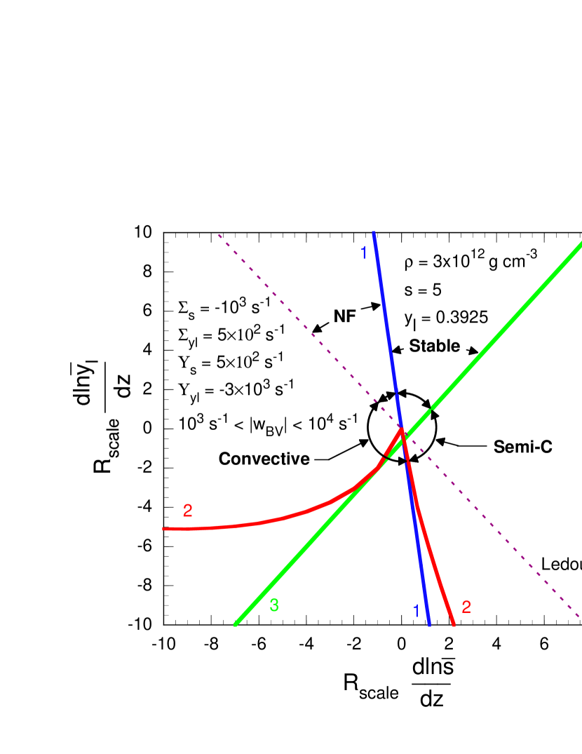
Nonzero values of the cross response functions, and , if non-negligible, can significantly affect the existence and location of the stable region, and the location and nature of the three unstable regions in the - plane. Figures 12 - 14 show cases in which the thermodynamic state, the value of the gravitational acceleration, and the two direct response functions, and , are the same as for the case shown in Figure 9, but the cross response functions have various nonzero values. The relatively small negative values given to and in Figure 12 cause the regions of stability and instability to be substantially shifted relative to that shown in Figure 9. Changing the sign of the cross response functions from negative to positive causes further shifts in the regions of stability and instability, as evident from a comparison of Figures 13 and 12.
Increasing the value of by an order of magnitude, which is more consistent with the numerical results for the response functions, leads to some interesting results. The stable region collapses to a very small sector about vertical axis, as shown by Figure 14, and several new modes of instability appear. Figure 15 shows a case for which the values of the response functions and the gravitational acceleration are the same as shown in Figure 14, but the thermodynamic state causes the derivative to be positive rather than negative. (This can arise for small values of , as discussed in Section 3.1.) It is seen that in this case the region of stability is reflected about the origin, and that again new modes of instability appear. As will be described below, these instabilities arise because of the substantial magnitudes of the cross response functions together the large ratio of to . These cross response functions cause a (a difference in between the fluid element and the background) to develop primarily in response to a (a difference in between the fluid element and the background). This is in contradistinction to the Ledoux case in which a develops from a displacement of the fluid element through a gradient in the background .
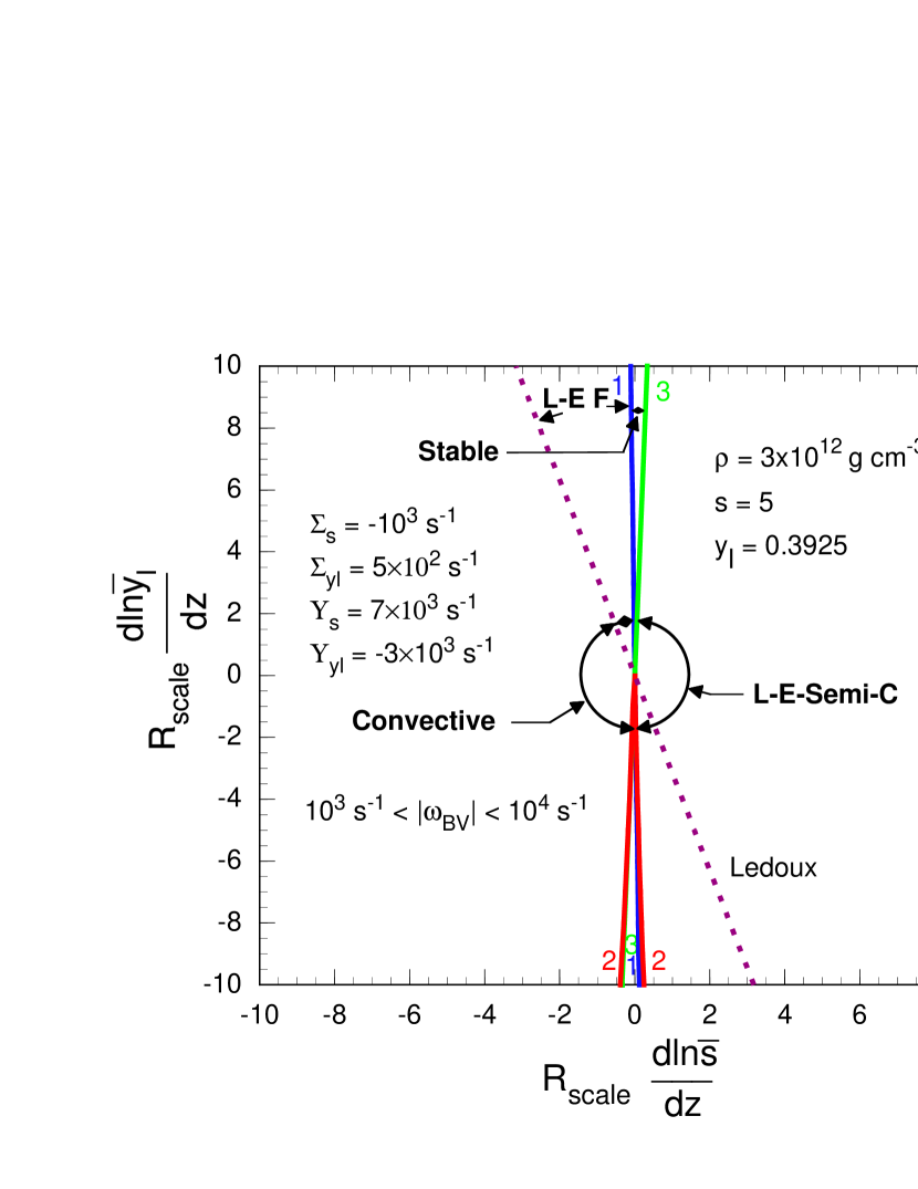
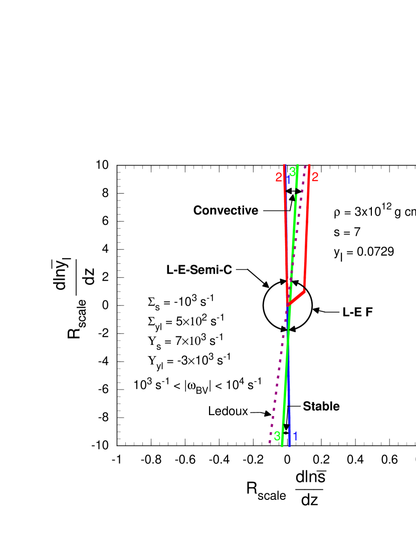
3.4.1 Lepto-Entropy Fingers (L-E-F)
We will discuss the instabilities that that are exhibited in Figure 15 here and in the next Section, and return to the instabilities exhibited in Figure 14 in Section 3.4.3. The instability on the right-hand side of Figure 15 denoted by L-E-F is new in that it has not been described or analyzed in the literature up to now. Moreover, it is likely to play the dominate role in producing convective-like fluid motions below the neutrinosphere of a proto-supernova. We begin by noting that the relative values of the response functions chosen for Figure 15 as well as the fact that are representative of these parameters in the region below the neutrinosphere and above the cold, unshocked inner core of a supernova progenitor. The relative values of the response functions seem to be generic, and will be discussed in more detail below. The positive value of is due to low values of which come about because the material in this region, unlike that in the cold inner core, encountered the shock and did so while still outside the neutrinosphere. This material therefore suffered extensive subsequent deleptonization when passing through the neutrinosphere by electron captures on the shock-dissociated free protons. The low values of the lepton fraction () and the moderately high values of the entropy () characteristic of this shocked material is the reason that , in accordance with Figure (3) and the discussion at the end of Section 3.1. Finally, the material in this region tends to have a positive entropy gradient, a relic of the shock ramping up through this region.
A positive gradient in , positive cross response functions, and a positive derivative can, under circumstances to be described, subject the region to an instability that we will dub “lepto-entropy fingers” (L-E F). This instability is thermal and lepton transport driven, as in the case of neutron fingers, but is very different from the latter. Recall that the neutron finger mechanism, to operate in the presence of a positive (stabilizing) entropy gradient and a destabilizing lepton fraction gradient, requires that thermal transport be much more rapid than lepton transport. The argument given for the presence of the neutron finger instability in proto-supernovae by the Livermore group, in fact, is based on the premise that thermal transport is rapid and lepton transport is negligibly slow. However, our results, which will be presented in detail in Section 6 and which span an extensive grid of thermodynamic states and fluid element radii show that typically . From the definitions of and , given by equations (6), this indicates that lepton transport is considerably more rapid than thermal transport, a fact noted by Bruenn et al. (1995) and Bruenn & Dineva (1996). The reason for this was pointed out in Bruenn & Dineva (1996) and is that the energy, , transported by a neutrino is limited by the rapid rise in neutrino opacity with , whereas a or a transports the same lepton number (viz., and for a and a respectively) independently of its energy. Furthermore, the and flows between a perturbed fluid element and the background can be oppositely directed, that is, additive in lepton number and subtractive in energy, depending on the temperature and the and chemical potential of the fluid element relative to the background.
Of critical importance in understanding the instability exhibited on the right-hand side of Figure 15, the lepto-entropy finger instability, is the fact that both and the cross response function are large and positive in magnitude, typically as large or larger than , and that the following inequalities are satisfied
| (59) |
where , , and can each denote either or . Thus, to operate in the presence of a positive (stabilizing) entropy gradient, lepto-entropy fingers requires lepton transport to be much more rapid than thermal transport, the opposite of the neutron finger requirement, and additionally requires that and that be large and positive.
The nature of the lepto-entropy finger instability can be illustrated by using inequalities (59) to simplify equations (9) - (11) to give
| (60) |
| (61) |
and
| (62) |
We have dropped the two small transport terms in equation (9) to get equation (60), and we have dropped and the last term on the right-hand side of equation (10) in comparison with the large and oppositely signed transport terms to get equation (61). Solving equation (61) for gives
| (63) |
where we have written equation (63) explicitly for the case in which and . Equation (63) together with equation (60) says essentially that the change of given by equation (60) is quasistatic compared with the rate at which the large transport terms and can adjust , and that will therefore adjust to the instantaneous value of as dictated by equation (63).
Equation (63) is critical to understanding the lepto-entropy finger instability, and the lepto-entropy semiconvective instability described in the next Section. While arises in response to a displacement of the fluid element through a gradient in the background entropy, as dictated by equation (60) and by the identical equation (13) for the familiar Ledoux case, arises in response to , as dictated by equation (63), rather than by a displacement of the fluid element through a gradient in the background lepton fraction, as dictated by equation (14) for the Ledoux case.
| (64) |
The derivative in equation (64) is always , but if the derivative , which occurs in the outer region of the core where is low as discussed above (e.g., Figure 3 and Figures 28 - 31), and if
| (65) |
then the fluid is unstable. For suppose, as an example, that . In the absence of transport this is a stabilizing gradient, for an outward displacement of a fluid element at constant entropy will result in which will make it more dense than the background and drive it back. Now, however, equation (64) with equation (65) satisfied asserts that will lead to an outwards acceleration of the fluid element, i.e., the fluid is unstable. A more mathematical statement of the above can be obtained by using equation (60) for in the derivative of equation (64) to get
| (66) |
which has growing solutions if and if equation (65) is satisfied.
How does this curious instability come about? A displacement of the fluid element through an entropy gradient results in a difference, , between the entropy of the fluid element and the background. The large value of means that the appearance of the entropy difference will quickly induce via equation (63) a lepton fraction difference, , between the lepton fraction of the fluid element and the background. The so induced is dependent only on , has the same sign as , and is independent of the gradient. Because and are of opposite sign, if the perturbation results in a restorative force, the induced perturbation will result in an anti-restorative force. If the induced perturbation is large enough relative to , the anti-restorative force wins out, and the perturbation grows, i.e., a “lepton finger” sustained by the entropy difference between the fluid element and the background will penetrate into the background. Thus, a Ledoux stable region can be destabilized by this diffusive lepto-entropy finger instability. Crucial to the emergence of the lepto-entropy finger instability is the large positive value of , and we shall illustrate by an example in Section 4 how this large positive value arises.
Despite the rather extreme assumptions that went into the derivation of inequality (65) (viz., , , , ), inequality (65) proves to be remarkably robust for predicting the lepto-entropy finger instability in proto-supernovae. In Section 6 we test this criterion for lepto-entropy fingers for one of the models we analyze by reducing to violate the inequality in equation (65) by 5 percent for every core radius and fluid element size for which it was satisfied, and find that the region previously found unstable to lepto-entropy fingers almost completely disappears.
The above analysis of the lepto-entropy finger instability breaks down when . An outward displacement will then result in a very small magnitude of and the last term in equation (10) involving the relatively large cannot now be neglected. Thus, there is a small sector about the vertical axis where which bounds the lepto-entropy finger region in Figure 15 where the fluid is either stable or convective.
3.4.2 Lepto-Entropy Semiconvection (L-E-Semi-C)
Consider now the case for which (Ledoux destabilizing) but for which the conditions leading to equation (64) are again satisfied (viz., , , , ). Then equation (66) as it stands gives stable oscillatory solutions if equation (65) is satisfied. However, the approximations leading to equation (66) are now inadequate, as the addition of even a small term in , due for example to the samll but nonzero values of and in equation (9), can, depending on its sign, turn the oscillatory solution of equation (66) into a damped oscillatory solution (stable) or a growing oscillatory solution (semiconvective). Equation (66) was obtained by approximating equations (9) - (11) by equations (60) - (62). To obtain a better approximation, we approximate equations (9) - (11) instead by
| (67) |
| (68) |
| (69) |
Here we have assumed, as in our analysis of lepto-entopy fingers above, that equation (10) is dominated by the transport terms and have dropped both the and the terms to get equation (68). Unlike our analysis of lepto-entopy fingers, however, we have retained the transport terms in equation (9) to get equation (67). Solving equation (68) gives as before
| (70) |
where we have written the last expression in equation (70) to explicitly account for the fact that and . Here as before the large values of the response functions and in comparison with the terms we have dropped guarantees that the value of adjusts immediately to the instantaneous value of . Substituting equation (70) into equation (69) gives equation (64) again, i,e.,
| (71) |
Taking the time derivative of equation (71) and using equation (67) for , we obtain in place of equation (66)
| (72) |
where we have used the equation (70) in obtaining the second expression of equation (72), and equation (71) in obtaining the last. Equation (72) is a more accurate version of equation (66) and differs from the latter in that some of the terms multiplying have been included. It will be used in place of equation (66) when the coefficient of are needed to decide between growing or decaying oscillatory solutions.
To continue our consideration of the case in which , rather than examining equation (72) it is conceptually easier to examine its first integral
| (73) |
We note first from equation (73) that if the coefficient of is greater than zero (i.e., , which, of course, requires that since ), then the solutions are oscillatory. The scenario here is analogous to that giving rise to lepto-entropy fingers discussed above. In fact, the same mechanism that destabilizes a fluid element in the presence of a stabilizing entropy gradient in the case above of lepto-entopy fingers, here tends to stabilize a fluid element in the presence of a destabilizing entropy gradient. Thus, an outward displacement of a fluid element through a negative entropy gradient results in the entropy of the fluid element becoming greater than that of the background, that is, a develops. This by itself would lead to a positive buoyancy force that would tend to force the fluid element farther outward. However, a induces a , in accordance with equation (70). If is large enough, i.e., if , then the negative buoyancy arising from together with a positive will overcome the positive buoyancy arising from , and the fluid element will be forced back. The fluid element will therefore oscillate.
Whether the oscillatory motion of the fluid element is growing or decaying depends on the sign of the coefficient of in equation (73). If this coefficient is less than zero, i.e., if , the solutions of equation (73) are decaying oscillatory and the fluid is stable. If , on the other hand, the solution of equation (73) is growing oscillatory and the fluid is unstable to semiconvection.
To examine the sign of further, we note that the response function is always negative. If the cross response function were zero, the coefficient of in equation (73) would be negative, the solutions would be decaying oscillatory and the fluid would be stable. This is analogous to the Schwarzschild stability described in Section 3.2 with . As pointed out there, an entropy perturbation, , and the buoyancy force it induces will be diminished by the tendency of neutrino transport (modeled by a negative ) to thermally equilibrate the fluid element with the background. Here the situation is similar except that the buoyancy force arising from an entropy perturbation, , comes about through the that it induces. In either case the effect of a is to reduce the buoyancy force with a phase such that a net work is extracted from the motion of the fluid element during the course of each oscillation.
However, if and additionally satisfies the inequality
| (74) |
then the coefficient of in equation (73) is , the solutions are growing oscillatory, and fluid is semiconvectively unstable. In this case, where both and are nonzero, there are two competing effects governing the growth or decay of the amplitde of oscillation of the fluid element. These are embodied by the two terms in the coefficient of in equation (73). The term, as described above, models the effect of an entropy difference on the thermal transport between the fluid element and the background viz., for the induced thermal transport drives a tending to reduce the magnitude of , and with it the buoyancy force. The effect is that a net work is extracted from an oscillating fluid element during the course of each oscillation. The term involving affects the motion more indirectly. It begins with the fact that an entropy difference, , induces a lepton difference, , in accordance with equation (70). This lepton difference, being, in turn, another driver of thermal transport between the fluid element and the background, as modeled by equation (67), provides a contribution to . This contribution has the same sign as if , which is usually the case. If inequality (74) is satisfied, the contribution to arising from the term involving is larger in magnitude than the contribution to arising from the term , and the net effect is a having the same sign as . With this, the oscillation amplitude of the fluid element grows. We thus have a case in which a lepton difference, , induced via equation (70) by an entropy difference, , does two things. It causes a growing mode to become oscillatory (the coefficient of in equation (73)), and it causes this oscillatory solution to grow (the coefficient of in equation (73)). We refer to this instability as “lepto-entropy semiconvection,” and denote it by “L-E-Semi-C” in the figures.
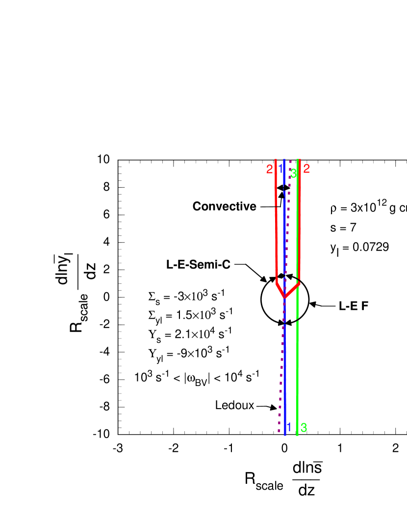
The condition for lepto-entropy semiconvection expressed by inequality (74) can be tested by reducing so that inequality (74) is no longer satisfied. Doing so for the response functions shown in Figure 15 required a substantial reduction in before the lepto-entropy semiconvective instability disappeared. However, the magnitude of response functions in Figure 15 are not large enough for the velocity term in equation (10) to be neglected in comparison with the diffusion terms. Increasing all of the response functions by a factor of three (equivalent to reducing the size of the fluid element) gives the results shown in Figures 16 and 17. Comparison of these two figures shows that lepto-entropy semiconvection is present for the case shown in Figure 16 in which inequality (74) is satisfied, but not in Figure 17 in which the inequality is not satisfied.

3.4.3 Lepto-Entropy Fingers and Lepto-Entropy Semiconvection in regimes where
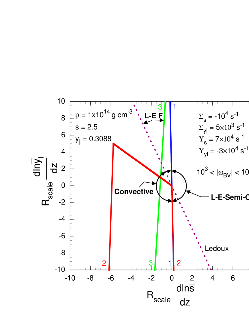
Another important case for proto-supernova is the case in which the conditions leading to equation (64) are again satisfied (viz., , , , ), but now , which occurs in the cold inner core where is high. Figure 18 shows the stability/instability regions in the - plane for a thermodynamic state representative of the colder and less highly deleptonized inner core where the above conditions are satisfied. The instabilities encountered here are similar to those exhibited in Figure 14, and the discussion here will therefore be applicable to the conditions shown in Figure 14.
To examine this case, we note that the conditions stated above imply that the approximations leading to equation (73) are satisfied here, and we rewrite this equation as
| (75) |
where we have explicitly exhibited the fact that now both and . Equation (75) gives a stability criterion similar to the Schwarzschild stability criterion of equation (32), viz., stable oscillatory solutions if and unstable solutions if . In the latter case, we have convection if we are in a region which is Ledoux unstable (most of the left-hand side of Figure 18), and lepto-entropy fingers in the region which is Ledoux stable (upper wedge on the left-hand side of Figure 18). The explanation for the presence of lepto-entropy fingers here is similar in origin to the case discussed in Section 3.4.1. Here a negative (destabilizing) gradient in is stabilized, in the absence of transport, by a sufficiently large positive gradient in depending on the relative magnitude of and . With transport, however, the lepton fraction difference, , between the fluid element and the background no longer arises from the displacement of the fluid element in a background gradient of , but in response to the entropy difference in accordance with equation (70), as in the case discussed in Section 3.4.1. Rather than stabilizing the fluid element, the induced with the same sign as , together with the negative value of , further destabilizes the fluid element, and we have a case which we will again refer to as lepto-entropy fingers.
The case in which is encountered frequently throughout much of the extent of the cold inner core of a proto-supernova. This positive entropy gradient arises during infall because the electron captures that take place in matter with increasing radius are more out of equilibrium due to a faster infall velocity of this matter. (Recall that the inner core collapses approximately homologously with infall velocity proportional to radius.) This causes an increased entropy production with radius.
A positive entropy gradient in equation (75) gives oscillatory solutions. In this case the entropy gradient is stabilizing, i.e., an outward displacement of the fluid element gives rise to a negative entropy difference, , which together with a negative gives rise to a negative buoyancy forcing the fluid element inward. A negative arises in response to the negative , in accordance with equation (70), and this together with the negative adds to the restoring force.
These oscillatory solutions are stable or semiconvective depending on whether the sign of the coefficient of in equation (75) is negative or positive, respectively. If the sign is positive, then the discussion at the end of Section 3.4.2 applies. In particular, an entropy difference drives a thermal diffusion which tends to reduce the magnitude of , damping the oscillation of the fluid element. But the that arises in response to , in accordance with equation (70), feeds back by driving a thermal diffusion tending to increase the magnitude of . If this latter thermal diffusion is large enough (i.e., if inequality (74) is satisfied) it dominates and causes the oscillation amplitude of the fluid element to grow. We then get a semiconvection driven by a induced by a , and we will refer to this case again as lepto-entropy semiconvection.
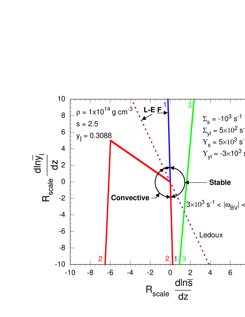
Referring back to Figure 18, the values of the response functions in this figure were chosen to satisfy inequality (74) but to otherwise be representative. Note that the region on the right (where ) is unstable to lepto-entropy semiconvection, in accordance with our discussion discussed above. As a test of the condition for lepto-entropy semiconvection as prescribed by inequality (74), Figure 19 shows the - plane for the same thermodynamic state and response function values as Figure 18 except that the value of the response function has been decreased from to so that inequality (74) is now violated. The region in the - plane unstable to lepto-entropy semiconvection in Figure 18 is now stable, validating the prescription given by inequality (74) for this case.
4. Computation of the Response Functions
In the preceding Section we discussed the effect of different sets of values of the response functions, , , and , on the locations of the stability and instability regions in the - plane, and on the modes of instability. In this Section we discuss how we obtain these response functions for a given thermodynamic state and fluid element size. Because the response functions depend on details of neutrino transport, and may be sensitive to these details, our approach is to compute the response functions by sophisiticated radiation-hydrodynamical equilibration simulations. The thermodynamic conditions (i.e., the values of the density , temperature , and lepton fraction ) of spherical fluid element are specified, and the size (radius) of the fluid element is chosen. The fluid element is then represented numerically by 20 spherical mass shells of equal width, and the background by 60 additional mass shells of the same thickness surrounding the fluid element. Initially the fluid element and the background are at the same thermodynamic conditions. The fluid element is then subjected to a perturbation in its thermodynamic conditions relative to the background, and the neutrino mediated re-equilibration of the fluid element with the background is then numerically computed. The radiation-hydrodynamical code used to perform these equilibration simulations is the same as that used to model core collapse and will be described in the next Section.
Two procedures, “isothermal” and “adiabatic,” for perturbing a fluid element relative to the background were tried. An isothermal perturbation proceeds as follows. Prior to performing the perturbation, the thermodynamic conditions of the fluid are frozen, neutrino interactions with the matter, but not transport, are turned on, and neutrinos are allowed to equilibrate locally with the fluid element and the background. The result is a uniform neutrino sea of all flavors in equilibrium with both the fluid element and the background. To complete the isothermal perturbation, the neutrino distributions are kept constant and the temperature or electron fraction or both of the fluid element are perturbed relative to the background, with the density of the fluid element adjusted so that pressure equilibrium between the fluid element and the background is maintained. In summary, an isothermal perturbation is a perturbation of the thermodynamic state of the fluid element relative to both the background and a uniform neutrino “sea.” To complete the simulation, neutrino transport is turned on. As the neutrinos re-equilibrate the fluid element with the background the radius, and therefore density, of the fluid is continually adjusted so that pressure equilibrium is maintained at all times. The results of this simulation are the time evolutions of the quantities and , where and are the entropy and lepton fraction mass averaged over the fluid element, and are the entropy and lepton fraction of the background, and and are defined at the beginning of Section 2.
An adiabatic perturbation begins with a perturbation of the temperature or electron fraction or both of the fluid element relative to the background. To complete the adiabatic perturbation, neutrino interactions with the matter, but not transport, are turned on, and neutrinos are allowed to equilibrate locally with the fluid element and the background. The result is that both the fluid element and the neutrinos within it are perturbed with respect to the background and the background neutrinos. Thus, an adiabatic perturbation is a perturbation of both the matter and neutrinos such that local thermodynamic equilibrium between the matter and neutrinos is maintained. Once the neutrinos have achieved local equilibration with the matter, neutrino transport is turned on and the re-equilibration of the fluid element with the background is followed. Pressure equilibrium between the fluid element and the background is maintained continuously by adjusting the radius (and therefore density) of the fluid element. As before, the results of this simulation are the time evolutions of the quantities and .
From a given simulation, time derivatives of the quantities and are computed by taking finite differences, i.e.,
| (76) |
where we have defined and to be the times required for and to be reduced to of their original perturbed values, respectively. Experiments showed that the choice of as a measure of the approach to equilibration in the determination of and was not critical, although the use of shorter time intervals gave slightly higher values for and , as would be expected.
To determine values of the response functions for a given thermodynamic state and fluid element radius, we performed two equilibration simulations beginning with different linearly independent sets of values of and for the perturbation of the fluid element with respect to the background. Call these two sets of perturbations and . We then took a linear combination of the two perturbations, choosing the coefficients and such that
| (77) |
and another linear combination, choosing and such that
| (78) |
From these linear combinations we compute the response functions. For example,
| (79) |
| (80) |
(Naturally it would have been possible to perturb at , and vice versa, and this would have made it unnecessary to chose linear combinations of the results. However, the procedure we adopted proved to be simpler to implement.)
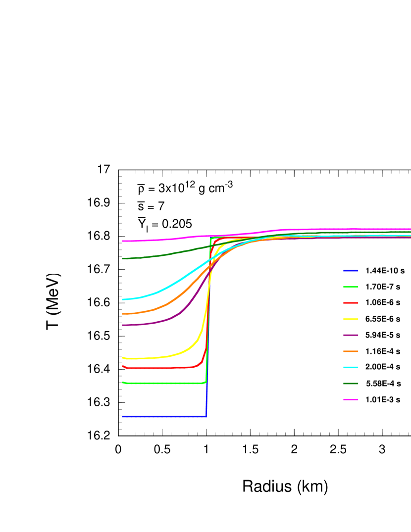
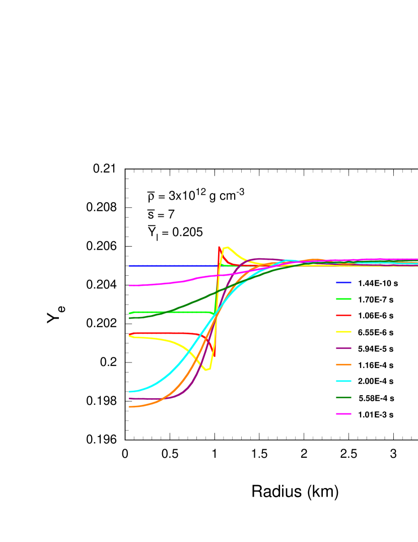
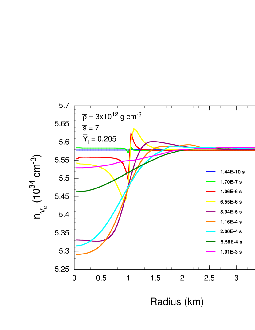
As we discussed above in Section 3.4, a large positive value of is critical to the emergence of the lepto-entropy finger instability. To illustrate how this comes about with a specific example, we show in Figures 20 - 25 some of the details of an equilibration simulation for an isothermal perturbation. The simulation was performed with improved neutrino rates. For ease of illustration, the state of the background that we chose, g cm-3, , , is a thermodynamic state for which the (and therefore ) chemical potential vanishes. The equilibrium and number densities in the background are therefore equal to each other. Because of this, it was possible to perturb the temperature of the fluid element and adjust its density to keep the pressure the same as the background while maintaining at its unperturbed value. (Different values of and number densities would have resulted in a perturbed value of in the fluid element after its density was adjusted to maintain pressure equilibrium, even if its value of was kept equal to that of the background.) While the choice of any other thermodynamic state would have illustrated our points, a choice which makes it possible perturb the temperature (and entropy) of the fluid element, maintain pressure equilibrium, and keep the value of at its unperturbed value provides the simplest and cleanest illustration of how a lepton fraction perturbation arises in response to an entropy perturbation, which is the basis of both the lepto-entropy fingers and lepto-entropy semiconvection instabilities.
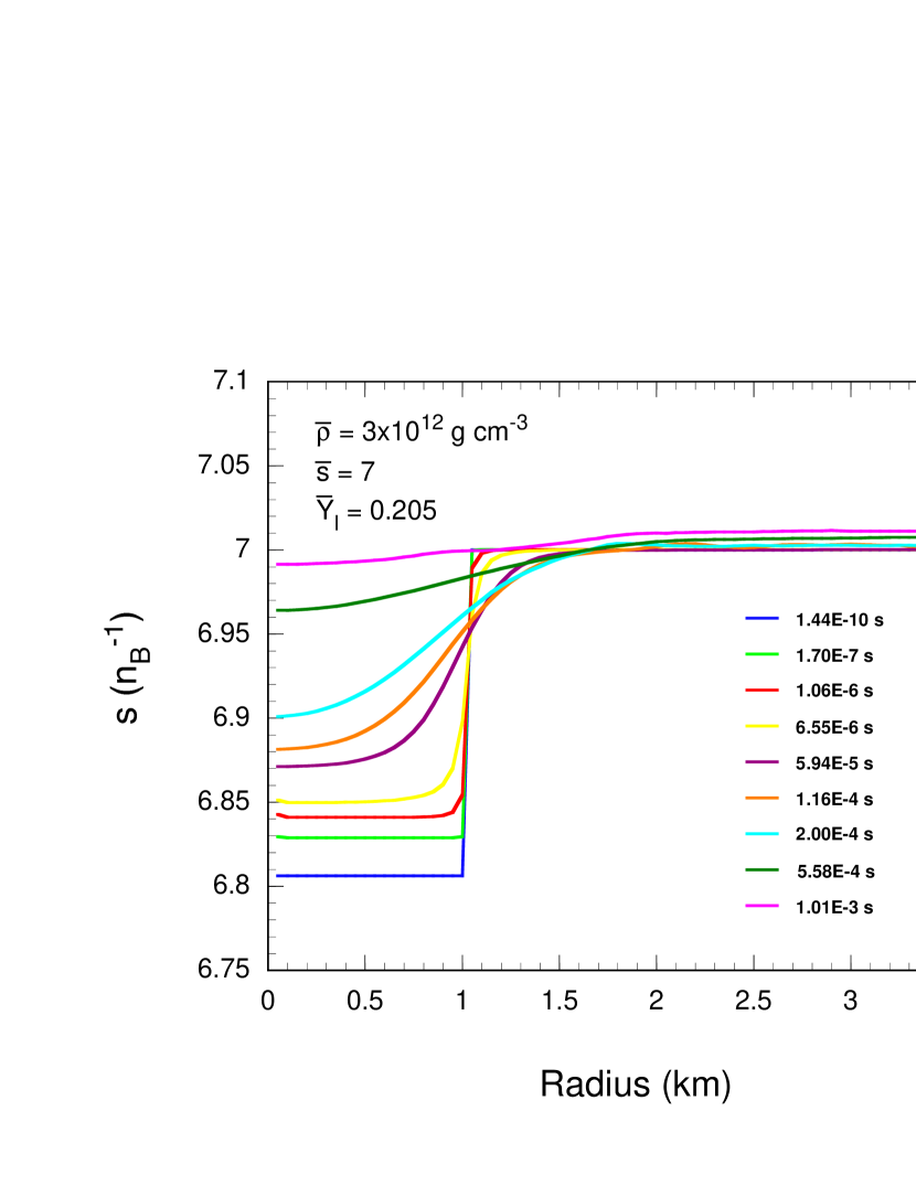
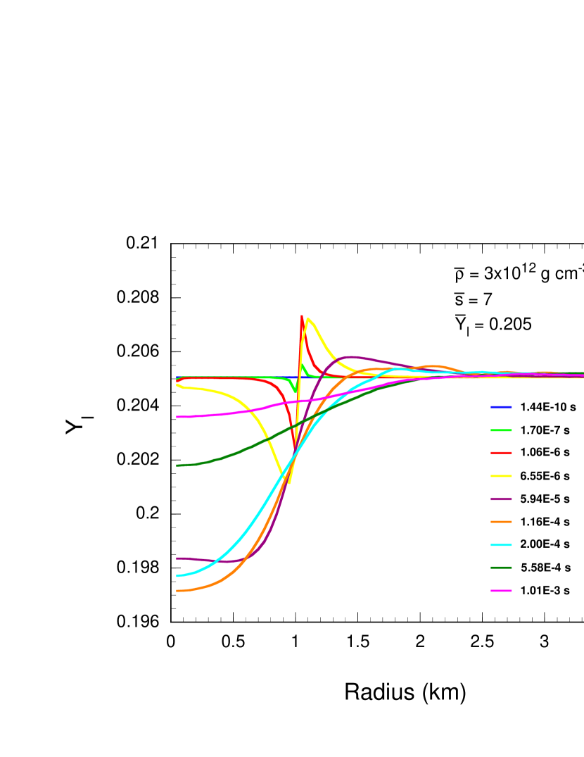
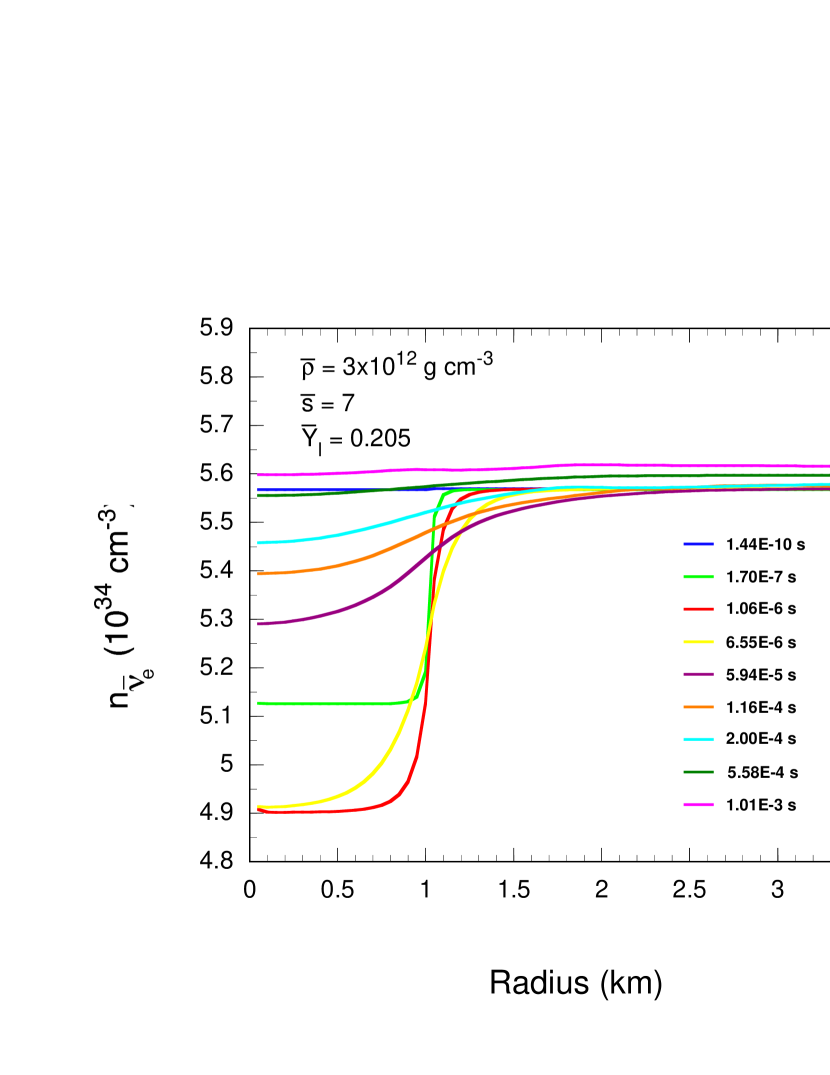
Figures 20 and 21 show the matter temperature and electron fraction profiles at selected times. The fluid element was perturbed relative to the background by decreasing its temperature, leaving the electron fraction unchanged, and adjusting the density to restore pressure equilibrium with the background. This initial perturbation is shown in the figures by the temperature and electron fraction profiles at the smallest time, . The above perturbation in results in the entropy perturbation shown in Figure 22 by the profile at . Because of our choice of a thermodynamic state with zero chemical potential, there is no net perturbation in the lepton fraction, as shown in Figure 23 by the profile at . As explained earlier in this Section, an isothermal perturbation is effected by first allowing the neutrinos to equilibrate locally with the fluid element and the background, both at the same thermodynamic state. The matter, but not the neutrinos, of the fluid is then perturbed. Thus, in particular, the electron neutrino and antineutrino number densities, and , are initially uniform when the matter is perturbed, as shown by the and profiles in Figures 24 and 25, respectively, at .
What happens almost immediately after the perturbation is that the ’s and ’s in the perturbed fluid element equilibrate locally with the matter, essentially establishing, thereby, conditions equivalent to an adiabatic perturbation. This is evident by comparing the and profiles at times s and s in Figures 24 and 25 with the corresponding profiles in Figures 26 and 27,. These latter figures show the time evolution of local the neutrino-matter equilibration with transport turned off so that only local equilibration can occur. It is seen that the profiles with transport turned on (Figures 24 and 25) and the corresponding profiles with transport turned off (Figures 26 and 27) follow each other closely, and that local equilibration is achieved in about 1 s. After this time the effects of transport begin to be seen, and the subsequent evolution is the same whether the initial perturbation is isothermal or adiabatic. This is why there is very little difference in the values of the response functions whether the perturbation is isothermal or adiabatic.
The local equilibration is very asymmetric, with decreasing by % versus a % decrease in , and this asymmetry is responsible for much of what follows. The asymmetry is due to the fact that the equilibrated values of and depend on electron number density, , and positron number density, , respectively, through the reactions and . The positrons are thermally produced as electron-positron pairs, so the value of is very sensitive to temperature and drops significantly with the temperature perturbation, whereas consists largely of fixed electrons (for the entropies of interest here), and is much less sensitive to temperature. Thus, while the perturbation of the fluid element reduces both and equally, the relative reduction in is much greater. The result is that the local equilibration of the ’s and ’s with the matter entails more absorption on protons (Figure 25, profiles at s and s) than absorption on neutrons (Figure 24, profiles at s and s), and this depresses (Figure 21, profiles at s and s).
After local equilibration, rapid lepton transport between the fluid element and the background adjusts the and distributions toward values for which there is a quasi net lepton flow equilibrium (i.e., a small ratio of net lepton flow to the flow in each direction) of ’s and ’s. Since the local matter-neutrino equilibration reduced the value of much more than that of , the difference between these two quantities drives a net lepton flow out of the fluid element, raising the value of and reducing that of (Figures 25 and 24, respectively, profiles at s, s, and s) until the establishment of a quasi net lepton flow equilibrium. The net flow of leptons out of the fluid element as a quasi net lepton flow is established reduces the value of in the fluid element (Figure 23, profiles at s, s, and s). At this point, then, there is a rapid reduction in the value of in response to the initial negative perturbation, , of the fluid element. This is the origin of the large positive value of , in accordance with its definition by equation 6, which is so crucial for the appearance of lepto-entropy fingers and lepto-entropy semiconvection.
After the establishment of a quasi net lepton flow equilibrium, the differences, and , between the values of and , respectively, between the fluid element and the background adjust as energy diffuses between the fluid element and the background, and slowly approach zero as the temperature of the fluid element equilibrates with that of the background on a relatively long timescale (Figure 20, profiles at s, s, s, and s).
In summary, an isothermal perturbation of the fluid element is followed by a local equilibration of matter and neutrinos on the shortest timescale, producing conditions equivalent to that of an adiabatic perturbation. Rapid lepton transport then adjusts the values of and on the next shortest time scale, establishing a net lepton flow equilibrium and producing thereby a lepton fraction difference, , in response to the initial entropy difference, . The slower thermal diffusion rate equilibrates the temperature of the fluid with the background on the longest time scale, while the lepton flow continually adjusts the values of and to maintain a quasi net lepton flow equilibrium between the fluid element and the background.
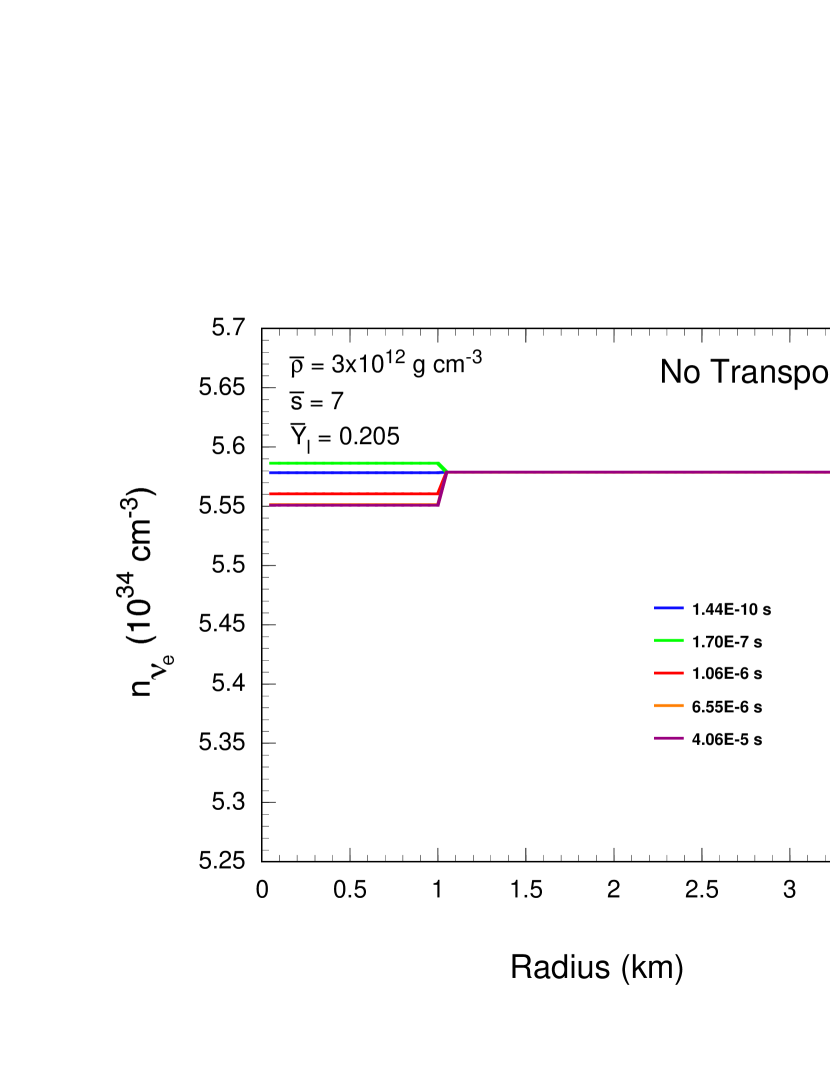
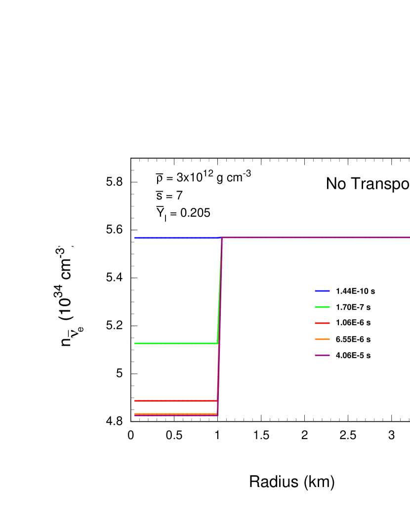
5. Core Collapse Models
As representative of the cores of supernova progenitors, we have chosen to examine at 100 ms and 200 ms after bounce the cores of a 15 (S15s7b) and a 25 (S25s7b) stellar progenitor. These were provided by Woosley (1995) and evolved from the main sequence to the onset of core collapse as described in Woosley & Weaver (1995). Precollapse model S15s7b has an iron core mass of 1.278 , representative of a small iron core mass progenitor, while model precollapse model S25s7b has an iron core mass of 1.770 , representative of a large iron core mass progenitor. Each progenitor was evolved through core collapse, bounce, and the shock reheating epoch by the code described in Bruenn (1985) and Bruenn & Haxton (1991), and extensively revised as described in Bruenn et al. (2001) and Bruenn (2003). The code is fully general relativistic. Neutrino transport is multigroup, three flavor and uses a flux-limited diffusion approximation. Twenty energy zones were used in these simulations spanning in geometric progression the neutrino energy range from 4 MeV to 400 MeV. The neutrino microphysics described in Bruenn (1985) and Bruenn & Haxton (1991) was used for the simulations, as well as some revised and new neutrino microphysics described below. Also used were the ion screening corrections given by Horowitz (1996) and implemented as described in detail in Bruenn & Mezzacappa (1997).
In some of the simulations, designated by “LS,” the Lattimer-Swesty equation of state (Lattimer & Swesty 1991) was used when the following three conditions were satisfied locally: (1) fm-3 ( g cm-3), where is the number density of nucleons (free and bound) per cubic Fermi, (2) MeV, and (3) the matter was assumed to be in nuclear statistical equilibrium (NSE). The Cooperstein-BCK equation of state (Cooperstein, 1985; Baron, Cooperstein, & Kahana, 1985) was used when the second and third condition was satisfied, but not the first. For nuclei not in NSE, which comprised the silicon layer, oxygen layer, and other exterior layers until they encountered the shock, seven alpha particle nuclei (plus neutrons and protons) were tracked explicitly. The nuclei were treated as an ideal gas (with excited states), and a nine-species nuclear reaction network was used to follow the nuclear transmutations. We will refer to this equation of state as the “non-NSE” equation of state. A zone not in NSE were flashed to NSE if its temperature reached 0.44 MeV (Thielemann, Nomoto, & Hashimoto, 1996). In order to compare our results more closely with those of the Livermore group, we also ran some of the simulations. designated by “W,” using the Livermore equation of state (Wilson, 2003). This equation of state was provided in tabular form. This W equation of state was joined smoothly to the non-NSE equation of state, and the latter was used when nuclei were not in NSE. Table 2 summarizes the core collapse simulations that were performed to produce the core configurations that will be analyzed in the next Section.
| Simulation | Progenitor | Equation of State |
|---|---|---|
| M15_LS | S15s7b | Lattimer-Swesty |
| M15_W | S15s7b | Livermore |
| M25_LS | S25s7b | Lattimer-Swesty |
| M25_W | S25s7b | Livermore |
For each of the models included in Table 2 the the stability of the fluid from the core center to the region just beneath the neutrinosphere was analyzed for two time slices, 100 ms and 200 ms after core bounce. The response functions, , , and , were obtained by performing equilibration simulations as described in Section 4 by the same code described above for the core collapse simulation. For most of the equilibration simulations, the “standard” neutrino microphysics described in Bruenn (1985) and Bruenn & Haxton (1991) was used, i.e., the same neutrino microphysics as used in the core collapse simulations. We observe, however, that neutrino physics has advanced beyond this standard. Recently, analytic expressions have been derived for neutrino absorption, emission, and elastic scattering on nucleons which take into account the nucleon recoil and blocking factors for arbitrary degeneracy (Reddy et al., 1998; Burrows & Sawyer, 1998, 1999). These new rates become smaller at high densities than the corresponding rates without nucleon blocking, and the recoil effects call into question the assumption that the scattering rates are isoenergetic. The latter will predominantly affect the thermalization of the ’s (by “’s” we refer to ’s and ’s and their antiparticles), as these particles lack the energy exchange channels of the charged-current processes on baryons which dominate the thermalization of the ’s and ’s. Thermalization simulations (Thompson et al., 2000), for example, show that -nucleon scattering is an important thermalization process for ’s with energies exceeding 15 MeV. Other neutrino processes that may be important for equilibrating a fluid element with the background are neutrino-nucleon bremsstrahlung and the related neutrino-nucleon inelastic scattering (Hannestad & Raffelt, 1998; Thompson et al., 2000).
We have performed equilibration simulations for several of the models with the improved (Reddy et al., 1998) absorption, emission, and elastic scattering on nucleons, and with the inclusion of bremsstrahlung and neutrino-nucleon inelastic scattering as formulated by Hannestad & Raffelt (1998). Models analyzed for stability using this improved neutrino microphysics are denoted by “Impr”, while those using the standard neutrino microphysics are denoted by “Stnd.” Table 3 lists the models analyzed for stability. We did not deem it necessary to include models obtained from core collapse simulations employing the improved neutrino physics because they differ very little below the neutrinosphere from those computed with the standard neutrino physics up to 200 ms after bounce. The improved neutrino physics mainly affects the luminosities and RMS energies of the ’s near and above the neutrinosphere. Furthermore, we wanted to perform the core collapse simulations with the Livermore equation of state and comparison models using the Lattimer-Swesty equation of state with neutrino microphysics as similar to that used by the Livermore group as possible.
| Model | Progenitor | Time from Bounce | EOS | -Microphysics |
|---|---|---|---|---|
| M15_LS_100_Stnd | S15s7b | 100 ms | Lattimer-Swesty | Standard |
| M15_LS_100_Impr | S15s7b | 100 ms | Lattimer-Swesty | Improved |
| M15_W_100_Stnd | S15s7b | 100 ms | Livermore | Standard |
| M15_LS_200_Stnd | S15s7b | 200 ms | Lattimer-Swesty | Standard |
| M15_W_200_Stnd | S15s7b | 200 ms | Livermore | Standard |
| M25_LS_100_Stnd | S25s7b | 100 ms | Lattimer-Swesty | Standard |
| M25_LS_100_Impr | S25s7b | 100 ms | Lattimer-Swesty | Improved |
| M25_W_100_Stnd | S25s7b | 100 ms | Livermore | Standard |
| M25_LS_200_Stnd | S25s7b | 200 ms | Lattimer-Swesty | Standard |
| M25_W_200_Stnd | S25s7b | 200 ms | Livermore | Standard |
6. The Stability of Collapsed Cores below the Neutrinosphere
Before analyzing the models listed in Table 3 for stability using the method described in the preceding Sections, let us first compare the core profiles produced by simulations using the Livermore equation of state with those produced by the Lattimer-Swesty equation of state, and ascertain the Ledoux unstable regions and the regions unstable to neutron fingers by the criteria given by the Livermore group (Wilson & Mayle, 1988). Recall that according to the Livermore group’s criteria a fluid is neutron finger unstable if a fluid element displaced outwards at constant composition but in temperature and pressure equilibrium with the background ends up after the displacement with a density less than that of the background. The profiles in entropy and lepton fraction of models M15_W and M15_LS are shown at 100 ms and 200 ms after bounce in Figures 28 and 30, respectively. Likewise, the profiles of models M25_W and M25_LS are shown at 100 ms and 200 ms after bounce in Figures 29 and 31, respectively.
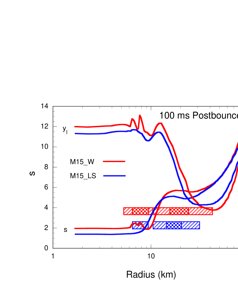
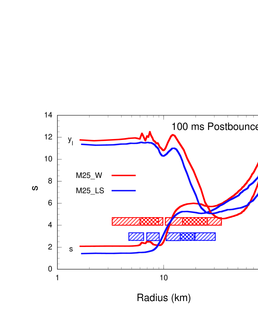
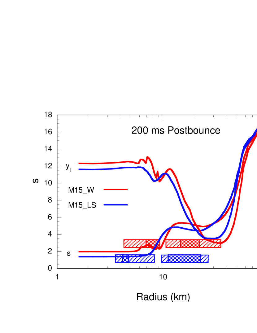
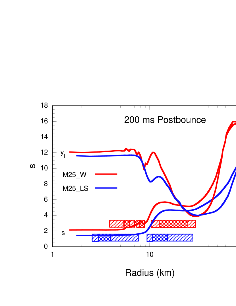
Figures 28 - 31 show that the core collapse simulations using the Livermore equation of state produce profiles in entropy and lepton fraction at 100 and 200 ms similar in shape to the simulations using the Lattimer-Swesty equation of state. The main differences are the slightly higher overall values of the entropy and lepton fraction given by the Livermore equation of state. These differences arise mainly during infall because of the smaller free proton fraction given by the Livermore equation of state in comparison with the Lattimer-Swesty equation of state for a given thermodynamic state. A smaller free proton fraction during infall leads to a reduced rate of electron capture, and this results in a higher lepton fraction at trapping. The electron captures that occur after trapping as the ’s equilibrate with the matter produces a greater increase of entropy, as the smaller free proton fraction and reduced electron capture rate given by the Livermore equation of state results in a greater disequilibrium between matter and ’s at trapping.
All models exhibit a region of Ledoux instability, indicated by the checkerboard patterns in the horizontal stripes, in the vicinity of 20 km from the core center at 100 ms, and models M15_W and M25_W exhibit an additional region of Ledoux instability in the vicinity of 8 km from the core center. At 200 ms the inward advection of matter has moved these Ledoux unstable regions slightly inward, and additional (very mild) Ledoux unstable regions have developed in models M15_LS and M25_LS at small radii. In most cases these Ledoux unstable regions are driven by negative entropy gradients. The location and even existence of these Ledoux unstable regions must not be taken very seriously, however, as convection, not included in these simulations, will rapidly smooth the entropy and lepton fraction gradients driving the convection.
Also shown in these figures by the slanted line pattern in the horizontal stripes are the regions that are neutron finger unstable by the Livermore group’s criteria. The neutron finger instability considerably extends the regions of fluid instability to either side of the Ledoux unstable regions. In particular, the region of fluid instability extends nearly up to the neutrinospheres, which are located near the outer parts of the troughs in the lepton fraction profiles. This illustrates the claim by the Livermore group that fluid motions resulting from the neutron finger instability will advect lepton rich matter to the neutrinosphere from regions below, and thereby enhance the luminosity.
Let us now consider the analysis of the models listed in Table 3 for stability using the methodology developed in the preceding Sections. To perform this analysis, each model was considered in turn and a double loop over the model was performed. The outer loop was over the spherical mass shells between the core center and the neutrino sphere (which comprised between 55 and 70 mass shells, depending on the model). For each mass shell the thermodynamic state and the gravitational acceleration were noted, and an inner loop was performed over the fluid element size. For this inner loop the radius of the fluid element was set initially to the flux-averaged mean free path for the mass shell under consideration and then increased successively by a factor of as the loop was executed until the radius of the fluid element exceeded one-half the distance of the mass shell from the center of the core. When the latter occurred, the loop was completed by setting the fluid element equal to one-half the distance of the mass shell from the center of the core. Thus, fluid element radii were considered spanning the range , where is the flux-averaged mean free path, is the radius of the fluid element, and is the distance from the core center to the mass shell in question. Executing this inner loop for each mass shell typically involved 6 to 12 fluid element radii. For each mass shell and fluid element radius two liinearly independent equilibration simulations were performed as described in Section 4. The results of this pair of equilibration simulations were the four response functions, , , and . Having computed these response functions, the gradients of and at the mass shell in question were noted, and the roots of equation (53) were obtained.
From these roots the stability of the fluid element of the given radius and at the given mass shell was ascertained as follows. If all the roots were real and negative, or if a real root was negative and the real part of a complex conjugate pair of roots was also negative, then the fluid was deemed stable for the given fluid element radius. If one or more of the real roots was positive, or if a real root and/or the real part of a complex conjugate pair of roots was positive, then the fluid was deemed unstable with a growth rate given by the largest of the positive elements, i.e., the largest of the real roots or the largest of the real root and the real part of a complex conjugate pair, as the case may be. If the largest positive element was the real part of a complex conjugate pair, and lepton transport dominated thermal transport (i.e., . which was always the case), the fluid was deemed unstable to lepto-entropy semiconvection for the given fluid element radius. If the largest positive element was a real root, the fluid would otherwise be stable in the absence of thermal or lepton transport (i.e., Ledoux stable), and lepton transport dominated thermal transport (again this was always the case), the fluid was deemed unstable to lepto-entropy fingers for the given fluid element radius. If the largest positive element was a real root, and the fluid would otherwise be unstable in the absence of thermal or lepton transport (i.e., Ledoux unstable), the fluid was deemed unstable to convection for the given fluid element radius.
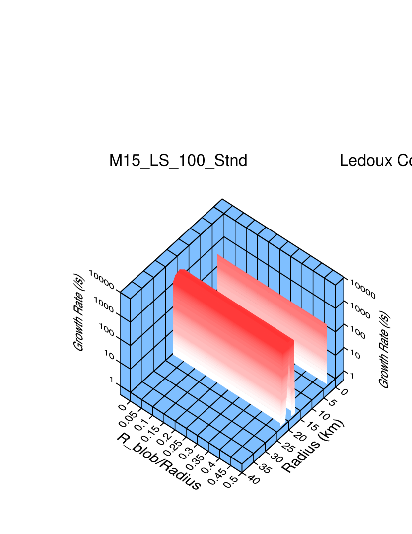
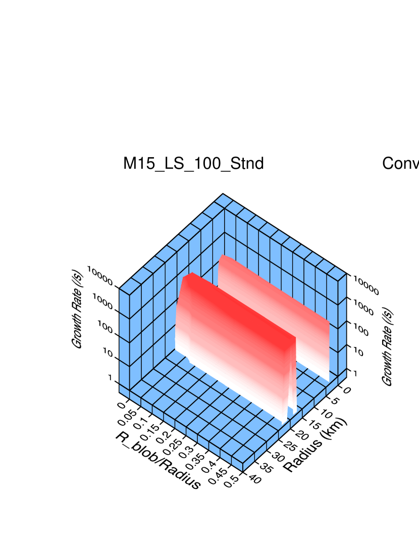


Figures 32 - 35 show the results of our analysis of the stability of model M15_LS_100_Stnd. Figure (32) gives the growth rate as a function of core radius and fluid element size for Ledoux convection, i.e., the growth rates of the fluid instability that would aeise in the absence of thermal and lepton transport. Except for an extremely narrow region near the core center, only the region between km and km is Ledoux unstable, where is the core radius, as is also evident from Figure (28).
Figure 33 gives the growth rates for the convectively unstable region, i.e., the region that is unstable in the presence of thermal and lepton transport that is also Ledoux unstable. The unstable convectively unstable region is essentially the same as the Ledoux unstable region, except that thermal and lepton transport slightly reduces the growth rates. This is because the convectively unstable region is buoyancy driven, and the tendency of thermal and lepton transport to equilibrate the fluid element with the background reduces the buoyancy that drives this convection.
Most interesting are Figures 34 and 35 which show regions that are unstable solely by virtue of thermal and lepton transport. Figure 34 shows that the lepto-entropy semiconvectively unstable regions are located toward the inner part of the core, i.e., between km and km. Referring to the discussion in Section 3.4.3 and Figure 18, instability to semiconvection is anticipated in the cold and relatively lepton rich inner core when the entropy gradient is positive, as it is for according to Figure 28. The lepto-entropy semiconvection will be dominated by small scales, as the growth rate for this instability increases with decreasing fluid element size, as is evident from Figure 34. Figure 35 shows the region unstable to lepto-entropy fingers. Significantly, it extends from the Ledoux unstable region to the vicinity of the neutrinosphere, and could be a very important source of lepton transport. The growth rates peak for fluid element radii near the neutrinosphere increasing in comparison with to deeper in the core.
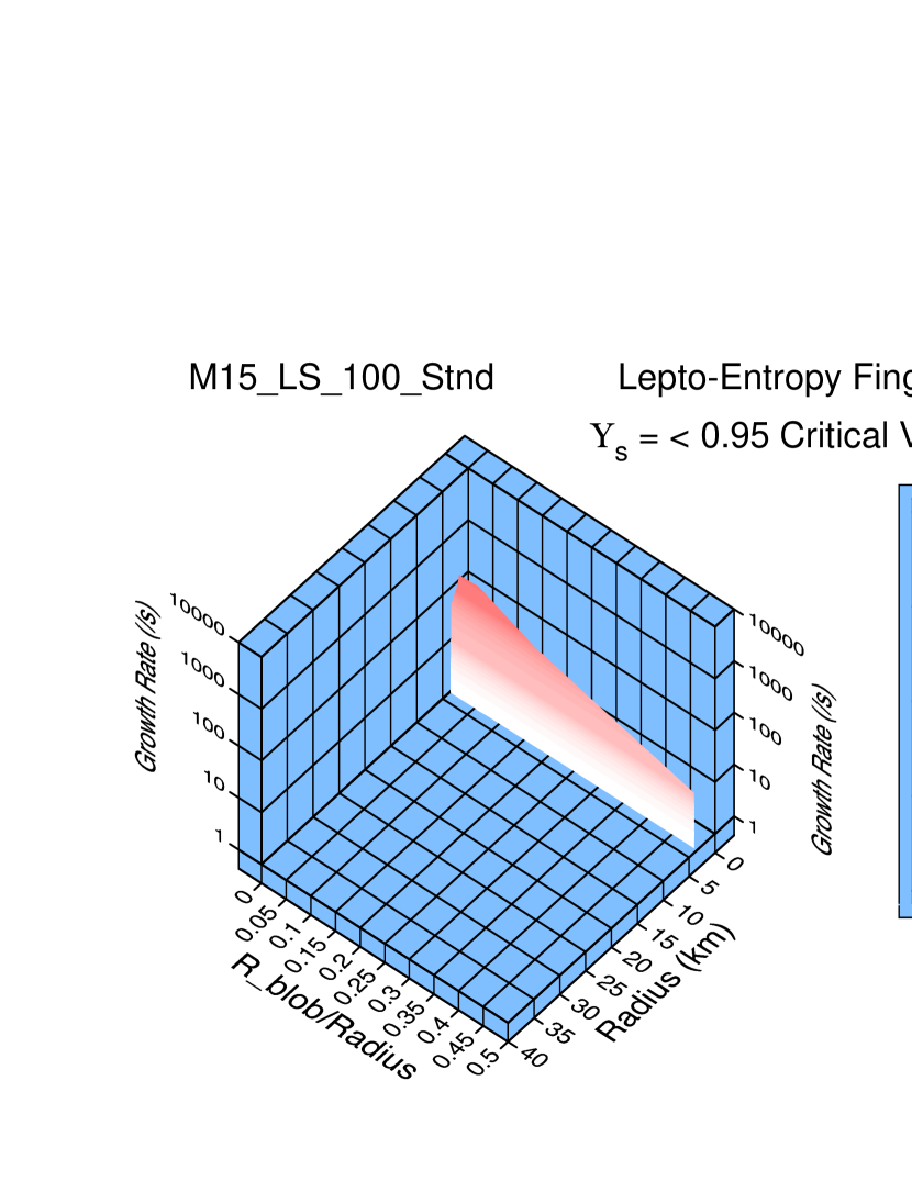
As a test of the applicability of inequality (65) in predicting the lepto-entropy finger instability in the collapsed cores of supernova progenitors, Figure 36 shows that when the cross response function is restricted to be no larger than 95 percent of the critical value, as given by the inequality in equation (65), the lepto-entropy finger instability disappears except for an insignificant region near the core center. Figure 36 provides a global view of the significance of inequality (65) for a particular core collapse model. Figures LABEL:fig:_st_pl_new1 and 38 provide an expanded view of the critical role of inequality (65) at a given thermodynamic state. These latter two figures show the plane for the thermodynamic state ( g cm-3, MeV, = 0.1165), which pertains to one of the zones of Model M15_LS_100_Stnd. The ratio of fluid element size to distance to core center (i.e., Rblob/Radius) was chosen to be 0.047, for which the lepto-entropy growth rate was maxmimum. Shown is the convective regions (red), lepto-entropy semiconvective region (green), lepto-entropy finger region (purple) and stable region (blue). Also shown are iso-growth rate contours. Figure 38
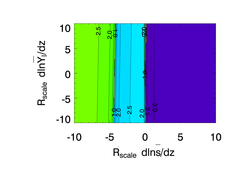
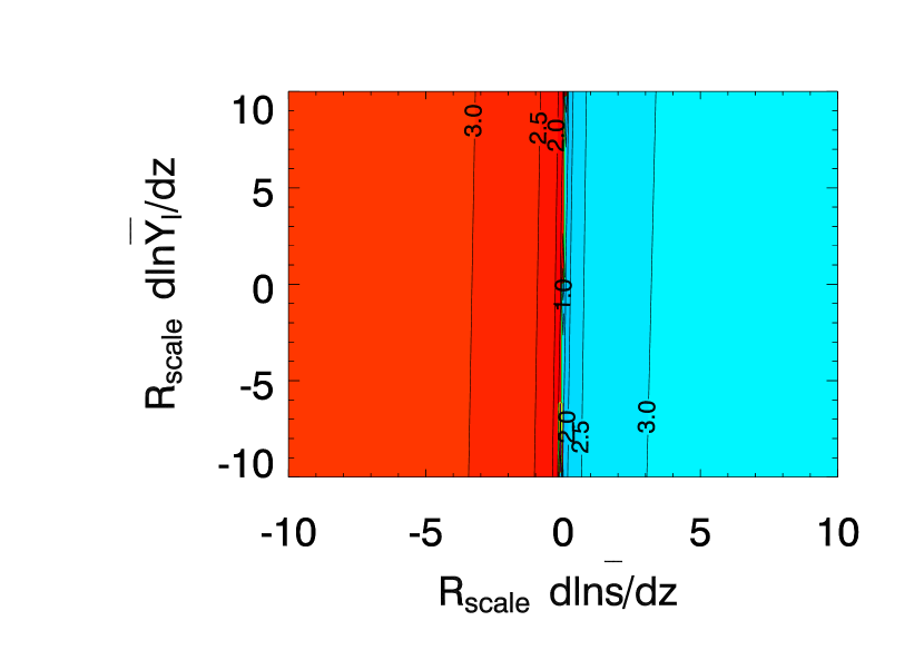
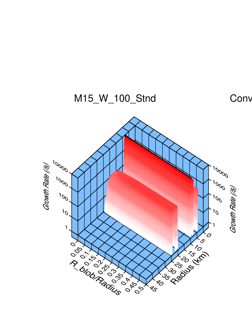
Figure 39 shows the regions of convective instability for model M15_W_100_Stnd, a model evolved with the Wilson EOS. There is a convectively unstable region deep in the core ( km), and another very narrow region near the core center. The convectively unstable region at km, not seen in model M15_LS_100_Stnd, corresponds to the negative gradients in both and , which can be seen in Figure (28), and which causes this region to be Ledoux unstable. Figures 40 and 41 show the regions of the lepto-entropy semiconvective and lepto-entropy finger instabilities, respectively. These regions are located in the core very similarly to the locations of the corresponding regions in model M15_LS_100_Stnd, except that the lepto-entropy growth rate is down by a factor of 2 or 3.
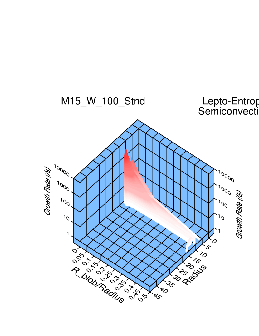
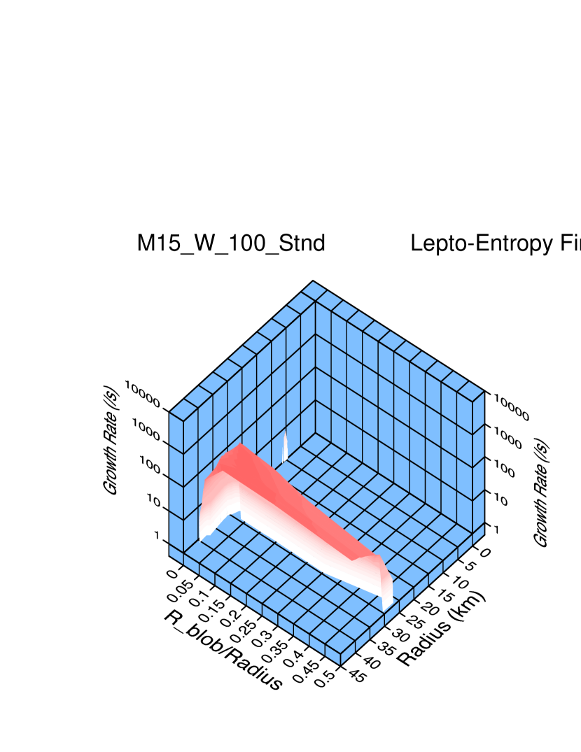
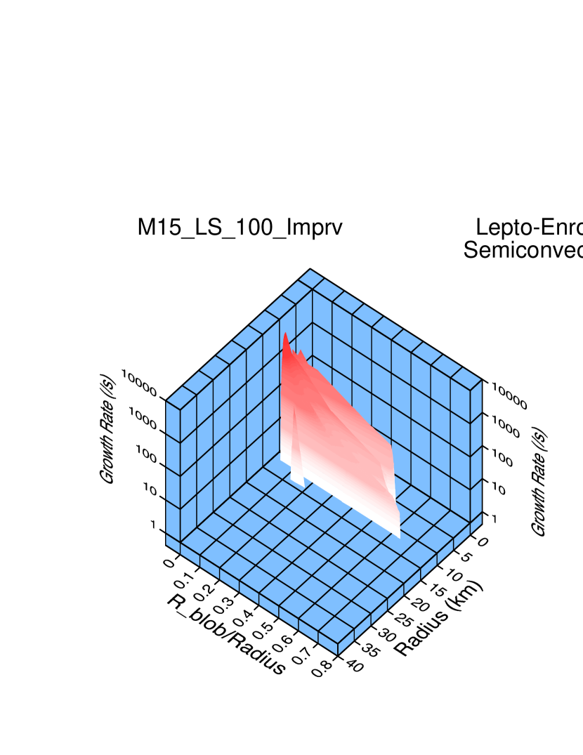

Figures 42 and 43 show the regions of lepto-entropy semiconvective and lepto-entropy finger instabilities, respectively, for model M15_LS_100_Imprv, a model whose regions and stability and instability were analyzed on the basis of “improved” neutrino microphysics. Lepto-entropy semiconvective is dominated at small scales, as in the case of the standard neutrino microphysics (Figure 34), but extends over a smaller region of , viz., km. Lepto-entropy fingers extends over a larger range of , from km up to the vicinity of the neutrinosphere, instead of from 23 km in the case of the standard neutrino microphysics. The lepto-entropy finger growth rates are about the same in both analyses, being about several hundred throughout most of the unstable region.
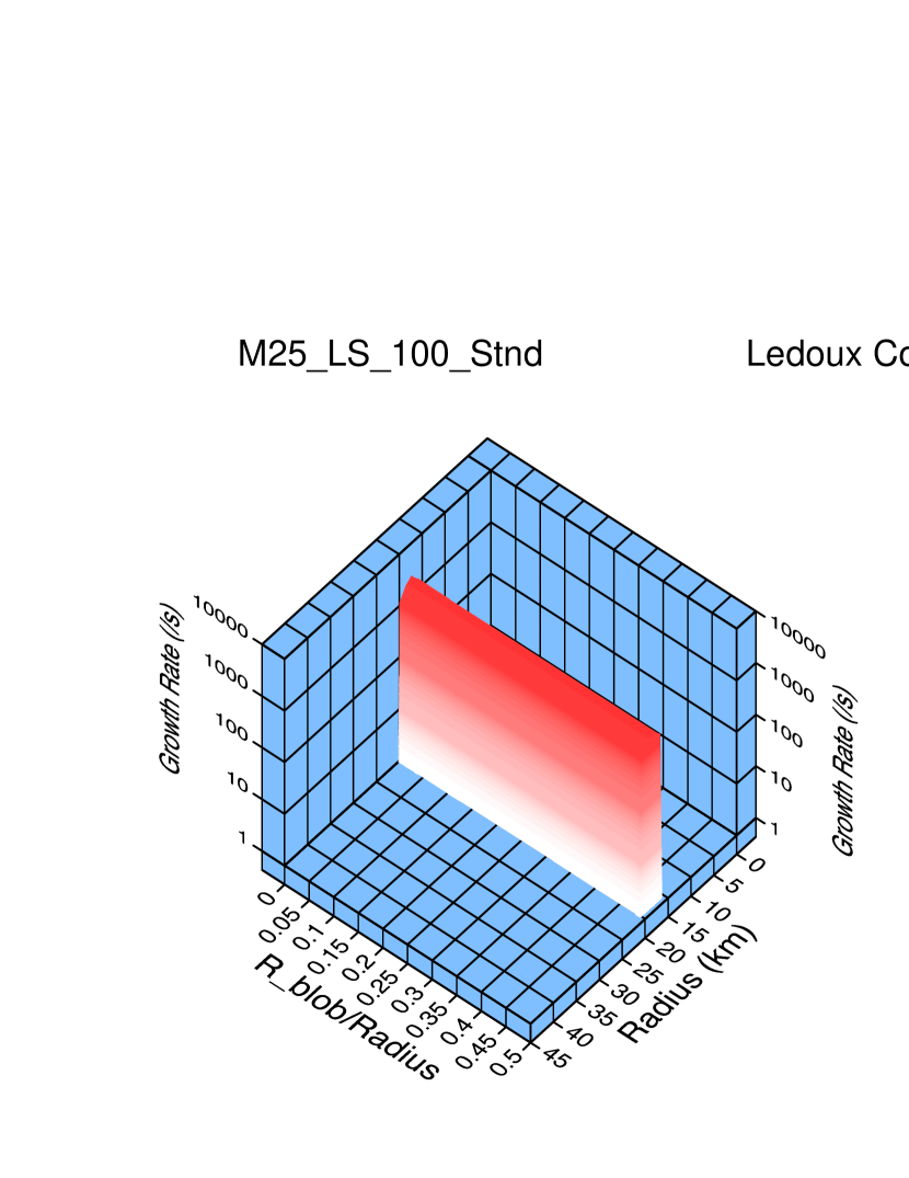
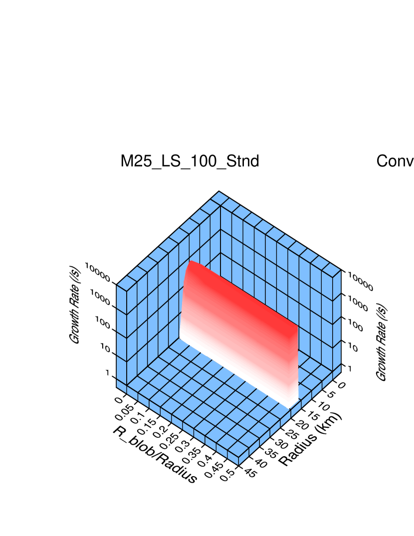
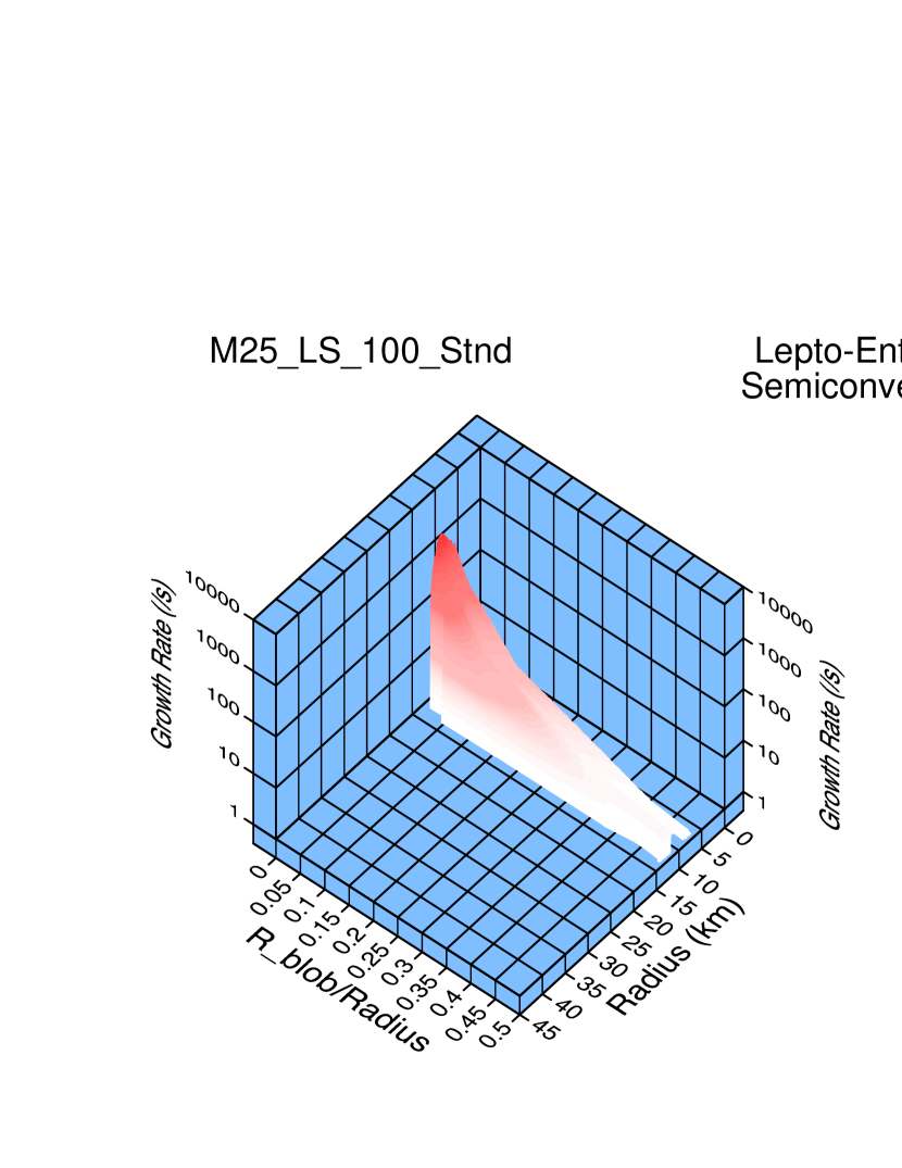
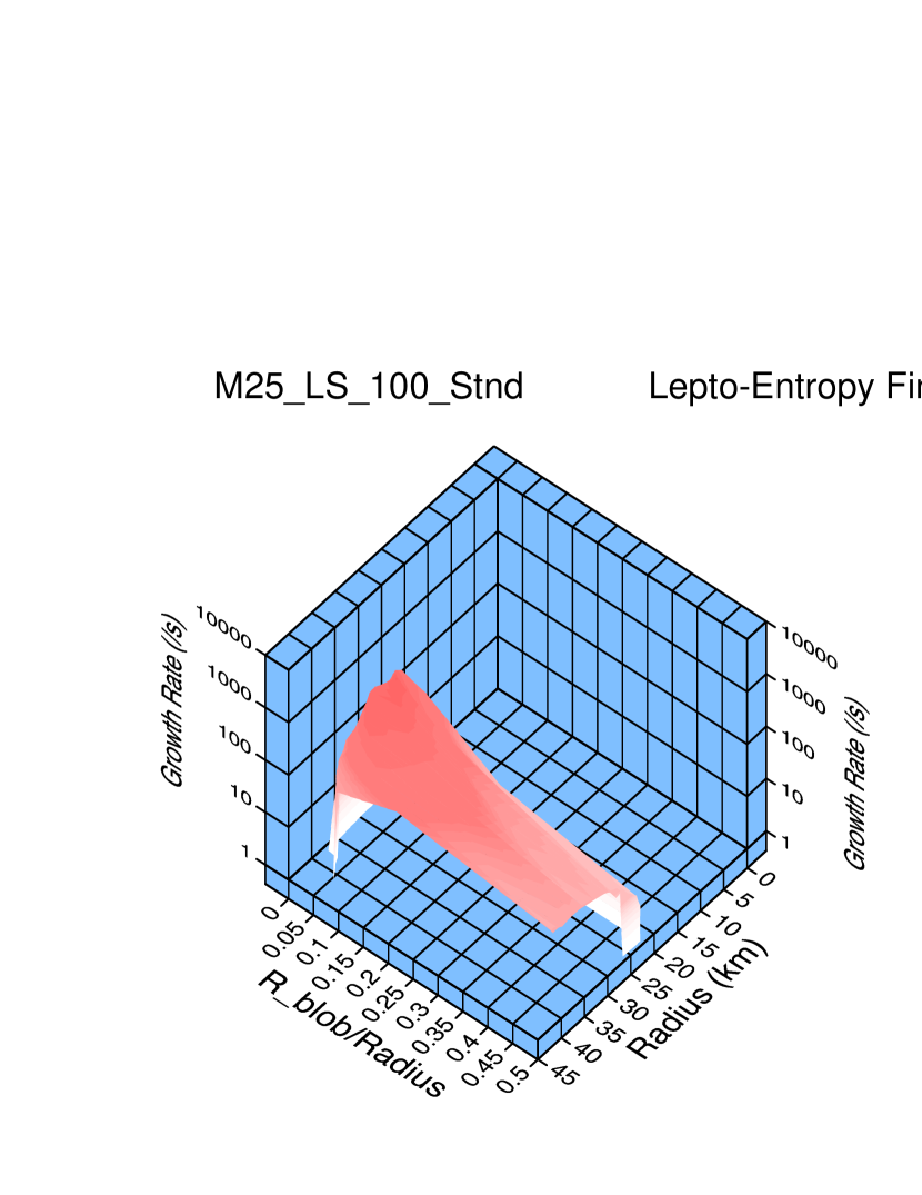
Figures 44 - 47 show the various instability regions for model M25_LS_100_Stnd and Figures 48 - 50 do the same for M25_W_100_Stnd (we omit the “Ledoux Convection” graph here because it is very similar to the “Convection” graph). Figures 52 and 52 show the regions of lepto-entropy semiconvective and lepto-entropy finger instabilities, respectively, for model M25_LS_100_Imprv (we omit the graphs of Ledoux Convection and Convection because they are very similar to the results for model M25_LS_100_Stnd. The graphs for models M25_LS_100_Stnd, M25_W_100_Stnd, and M25_LS_100_Imprv_NF are similar, respectively, to the corresponding graphs for models M15_LS_100_Stnd, M15_W_100_Stnd, and M15_LS_100_Imprv_NF. The various modes of instability are qualitatively in the same regions of the core, and the growth rates of these instabilities are similar.
We omit showing graphs of the various instability regions for the models at 200 ms as it is not clear how meaningful they are at this time. The fluid motions resulting from the instabilities would have modified the background gradients in and , thus modifying the instabilities and their growth rates. Indeed, they may already have done so by 100 ms. All that can be said without detailed multi-dimensional radiation-hydrodynamical simulations is that the lepto-entropy semiconvective and lepto-entropy finger instabilities are likely to appear for for some period of time after core bounce below the neutrinosphere of a proto-supernova.
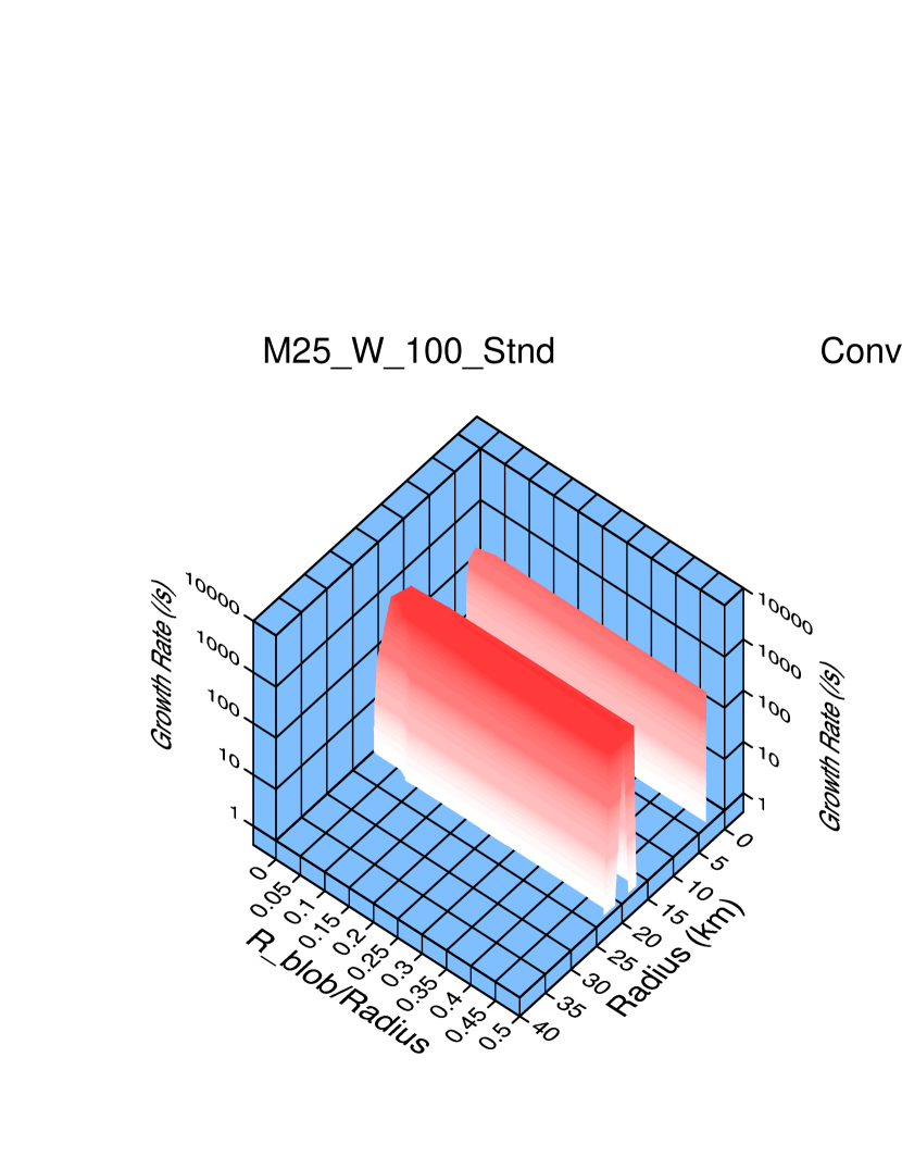
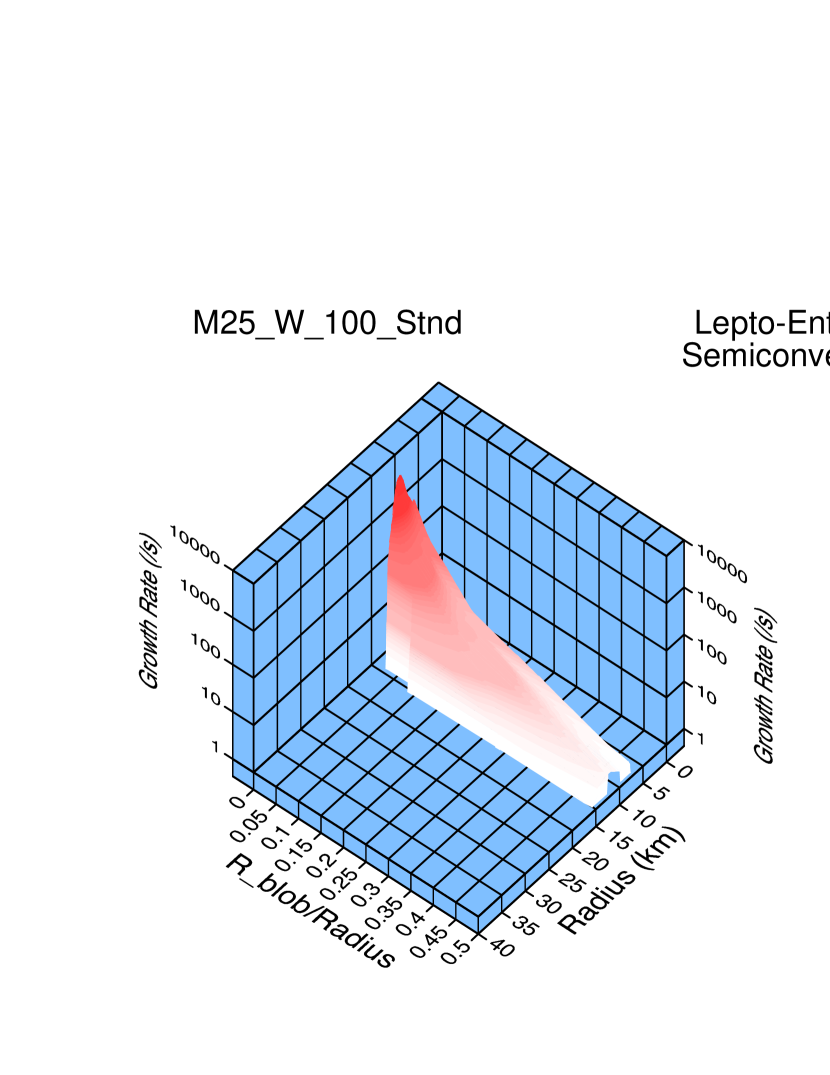
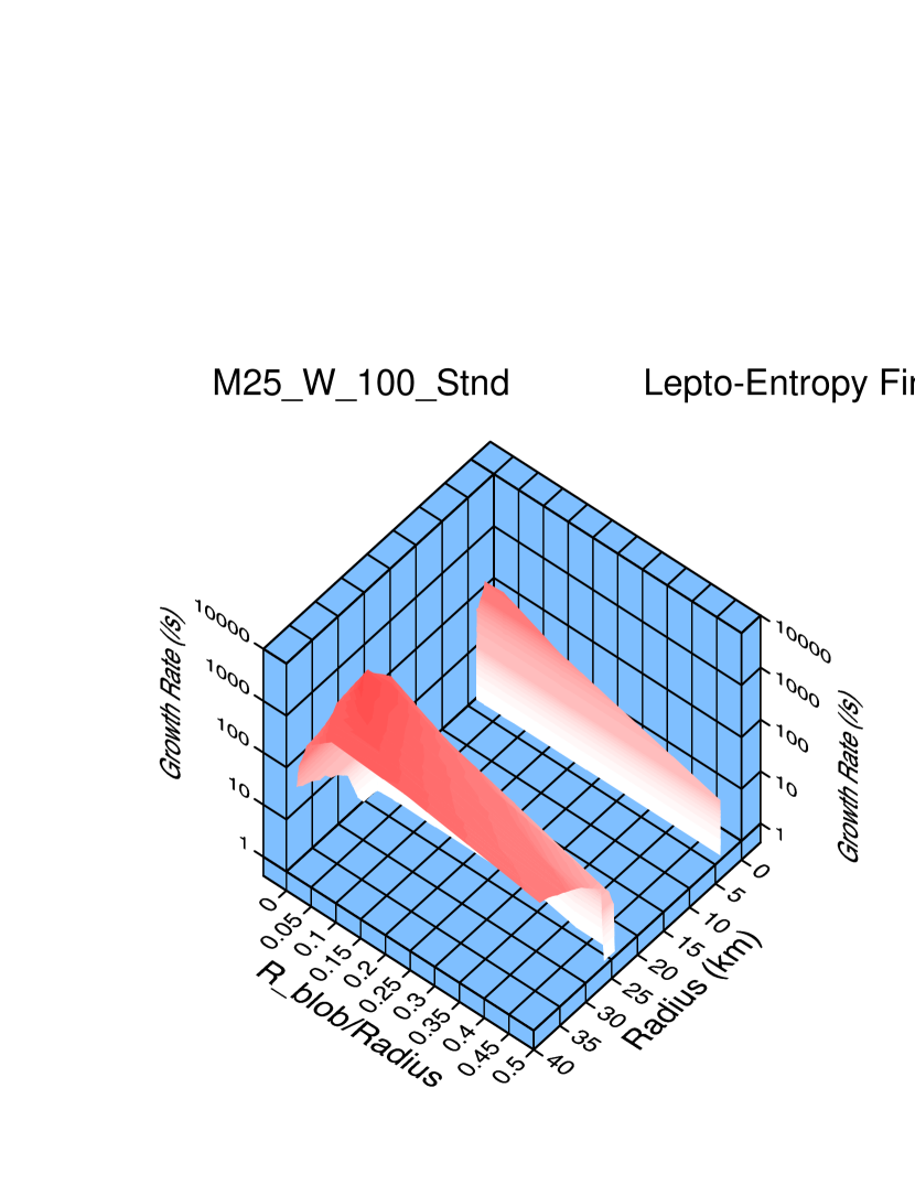
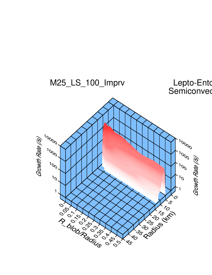
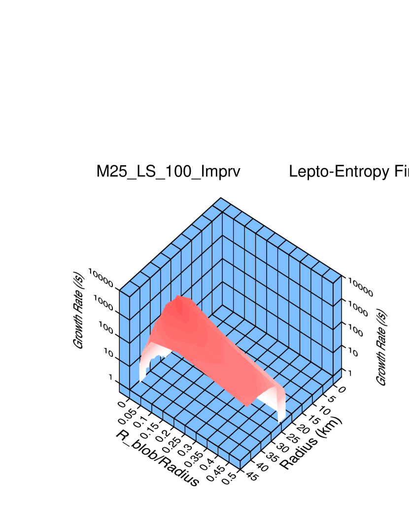
7. Comparisons With Other Work
In this Section we will compare our the results of stability analyses with the few other analyses of doubly diffusive instabilities in the literature that are relevant to the collapsed cores of supernova progenitors, and we will examine results of extant multi-dimensional radiation hydrodynamical simulations of stellar core collapse to see if the lepto-entropy finger instability has been seen in any of these simulations
7.1. Comparisons With Prior Stability Analyses
A number of authors have recognized the potential role of convection below the neutrinosphere in enhancing the neutrino luminosity. Most of this work e.g., (Epstein, 1979; Bruenn et al., 1979; Livio et al., 1980; Colgate & Petschek, 1980; Smarr et al., 1981; Lattimer & Mazurek, 1981; Burrows & Fryxell, 1993; Janka & Müller, 1993, 1994; Bruenn & Mezzacappa, 1994; Keil et al., 1996), was focussed on Ledoux convection or Raleigh-Taylor overturns. Smarr et al. (1981) pointed out the possibility of doubly diffusive instabilities, in particular, neutron fingers, arising in the core after bounce. The Livermore group (Wilson et al., 1986; Wilson & Mayle, 1988, 1993) have emphasized the role of doubly diffusive instabilities below the neutrinosphere and have incorporated it in their simulations. In their treatment of these instabilities, they have assumed that the rate of thermal equilibration greatly exceeds that of lepton equilibration, using arguments reviewed in Section 1, and on the basis of this found that material below the neutrinosphere in their core collapse simulations was unstable to neutron fingers in an extensive region. Modeling the resulting convection by a mixing length algorithm they found an enhancement of the luminosity which helped power explosions in their simulations.
Bruenn et al. (1995) applied the single particle analysis of Grossman et al. (1993) to stellar material with neutrino mediated thermal and lepton transport. On the basis of some numerical equilibration experiments they questioned the assumption that thermal equilibration rate exceeded the lepton equilibration rate, and concluded that the neutron finger instability would probably not be present in the collapsed cores of supernova progenitors. They also rediscovered the the observation of Lattimer & Mazurek (1981) that the derivative changes from negative to positive when the value of falls below a critical value, and that the core was likely stable when that occurred.
Bruenn & Dineva (1996) also applied the single particle analysis of Grossman et al. (1993), and extended the analysis by introducing the four response functions and the methodology for determining their values. They also pointed out that the rate of lepton transport substantially exceeded the rate of thermal transport, and that the appearance of neutron fingers in the collapsed core of a supernova progenitor was very unlikely. Like Bruenn et al. (1995), however, they applied their analysis to only a very limited region of the thermodynamic state space of a core and concluded that the material would either be semiconvective or stable, depending on the value of .
Miralles et al. (2000) have examined the stability of the material in an evolving protoneutron star. By employing an equilibrium diffusion approximation for neutrino transport they were able to derive a dispersion equation (a cubic equation analogous to equation (53)) involving both the growth or decay rate and the horizontal wave number or length scale of the perturbation. They were thus able to solve for the length scale of a perturbation giving the minimum thermal and lepton gradients needed for instability or, equivalently, the length scale of a perturbation giving the maximum growth rate for given thermal and lepton gradients. In our work it was necessary to consider different length scales explicitly. However, the use of an equilibrium diffusion approximation for neutrino transport may cause some of the subtleties of the transport to be missed and result in different relative values for the response functions.
The Miralles et al. (2000) analysis was applied to the interior of a neutron star during its long term evolution. Their results are therefore probably not directly comparable to the results of our analysis here which pertain to the collapsed cores of supernova progenitors before the excess entropy of the shocked material has had a chance to be radiated away. Nevertheless we note that very early in the evolution of the protoneutron star studied by Miralles et al. (2000) they find a convectively unstable region near the surface surrounded by diffusively unstable region which they attribute to neutron fingers. They do not find semiconvection anywhere. This appears to be not altogether dissimilar to our results which show a convectively unstable region bounded above by lepto-entropy fingers and below by semiconvection. The appearance of semiconvection below the convectively unstable region in our models and not in the model examined by Miralles et al. (2000) might be due to the fact that the lepton fraction in the deep interior of our models is relatively large (so that whereas the opposite might have been true in their model. According to the discussion at the end of Section 3.4, this could explain the different results.
The Miralles et al. (2000) work also included viscosity, the magnitude of which is uncertain and not included in this work, They found that viscosity, as given by van den Horn & van Weert (1981), did not greatly affect the diffusively unstable regions, but found that the convectively unstable regions to be more extended with the inclusion of viscosity..
The role of magnetic fields in the development of proto-neutron star instabilities was investigated in Miralles et al. (2003). Magnetic fields have a dual role: stabilization and destabilization. The essential results presented in Miralles et al. (2003) indicate that magnetic field strengths in excess of G may do both: stabilize regions unstable to convection, limiting the spatial extent of such regions, and destabilize regions to new modes of instability. However, their fundamental conclusion is that only very strong magnetic fields ( G) would significantly alter the stability properties of proto-neutron stars. These fields might be generated by dynamo action from convective activity present in the core prior to the escalation of field strengths. Once the field strength increases, convective activity is shut off. Thus, magnetic fields may affect both the spatial extent and the temporal duration of convective activity in the proto-neutron star.
7.2. Comparisons With Multi-Dimensional Core Collapse Simulations
Most of the extant multi-dimensional radiation-hydrodynamical simulations of stellar core collapse have employed gray neutrino transport, and it is not clear how much of the dynamics of the lepto-entropy finger instability these simulations are capable of capturing. With this caveat in mind, we will proceed to examine the results of these simulations that have been described in the literature.
The simulations of Herant et al. (1994) used a smooth Newtonian two-dimensional SPH (smooth particle hydrodynamics) code coupled to gray neutrino transport. The letter transports number of energy of each neutrino species in a two-part scheme consisting of flux-limited diffusion scheme for optically thick regions and a light bulb approximation for optically thin regions. For their core collapse simulation of a 25 Weaver and Woosley Weaver & Woosley (1993) an instability below the neutrinosphere developed over a time scale of 15 ms after bounce with maximum turnover velocities varying over time between 1000 and 4000 km s-1. This unstable region extended 15 km below the neutrinosphere which had a radius of 40 km at the time, with 5 convective cells in a 90 degree sector. Herant et al. (1994) attributed this instability to the neutron finger mechanism described by the Livermore group. The time for the growth of the instability, the scale of the turbulence, and the region over which it was observed is consistent with the results displayed in Figure 35. We suggest that they were seeing lepto-entropy fingers.
The simulations of Fryer (1998, 1999), and Fryer & Warren (2002) used basically the smooth Newtonian dimensional SPH code coupled to gray neutrino transport of the Herant et al. (1994) work, but with improvements in the SPH code (e.g., technical improvements and the addition of GR effects), the equation of state, and the neutrino transport (the latter still being gray, however). Additionally. the simulations performed perfromed by Fryer & Warren (2002) were three-dimensional. Unfortunately most of the discussion in these works was concerned with the entropy driven convection occurring above the neutrinosphere, rather than convection below. However, Figure 2 of Fryer & Warren (2002), which is a two-dimensional slice of the core of a 15 progenitor 75 ms after bounce, does show evidence of convective flows below the neutrinosphere, although it is difficult to infer details.
Both the simulations of Miller et al. (1993) and Janka & Müller (1996) cut out the innermost part of the collapsed stellar core and imposed boundary conditions, so fluid motions below the neutrinosphere were not computed. In the simulations of Mezzacappa et al. (1998a), a PPM hydrodynamics scheme was coupled to the zero and first moments of neutrino fields previously computed in spherical symmetry with a multigroup, flux-limited transport. While these simulations were able to capture some convective instabilities, the imposed neutrino background resulted in the inability of simulations to compute the fluid element-to-background neutrino transport that would arise in response to differences between the thermodynamic state of the fluid element and the background. Consequently, doubly diffusive instabilities could not be captured by these simulations.
Finally, the simulations of Buras et al. (2003) used Newtonian PPM hydrodynamic with some general relativistic corrections coupled to radial-ray transport via a multigroup, tangent ray scheme with closure provided by the solution of the Boltzmann equaiton on an angularly averaged stellar background. While details are sparse, the authors describe a convection that sets in below the neutrinosphere by 40 ms after bounce, is persistent up to 0.26 s after bounce when the simulations were terminated, and which slowly extended deeper into the core. The authors attributed this convection to Ledoux convection, but it may have been lepto-entropy fingers.
8. Conclusions
The fluid below the neutrinosphere of the collapsed core of a supernova progenitor can be driven unstable by thermal and lepton diffusion as well as by a gravitationally unstable stratification of the fluid. We have developed the methodology introduced by Bruenn & Dineva (1996) for analyzing fluid instabilities in the presence of neutrino mediated thermal and lepton transfer. In this analysis four “response functions” are introduced to model the thermal and lepton equilibration of a fluid element perturbed in entropy and lepton fraction from that of the background. These response functions depend on the thermodynamic state of the background and the size of the fluid element, and are obtained by detailed neutrino transport simulations. Given values of the response functions and the ambient gravitational field at the position of the fluid element, a cubic equation can be derived whose roots characterize the response of the fluid element to a perturbation in either its motion or thermodynamic state. From a determination of these roots, the stability or mode of instability of the fluid can be ascertained as a function of the gradients in entropy and lepton fraction. This methodology is applied both to resolve a long standing controversy regarding the presence of the neutron finger instability below the neutrinosphere, and to perform an extensive analysis of the fluid instabilities that do occur below the neutrinosphere for a number of representative post bounce supernova progenitors.
The Livermore group (Wilson et al., 1986; Wilson & Mayle, 1988, 1993) have argued that thermal equilibration proceeds much more rapidly than lepton equilibration in the fluid below the neutrinosphere. As a consequence, given the gradients in entropy and lepton fraction that arise in their supernova models subsequent to the initial collapse of the core and bounce they found that the neutron finger instability will arise in an extensive region below the neutrinosphere. Modeling by a mixing length algorithm the fluid motions that are expected to result from this instability, they found an enhancement of the luminosity that helped to produce successful explosions in their sophisticated spherically symmetric supernova simulations. Their work is very important as it has emphasized the potential role of fluid instabilities below the neutrinosphere in the supernova mechanism.
We have performed core collapse simulations using the Livermore (Wilson, 2003) equation of state. Applying their criteria for the neutron finger instability, we do find an extensive region below the neutrinosphere, on either side of a Ledoux unstable region, that is neutron finger unstable. A similar exercise for core collapse simulations computed with the Lattimer & Swesty (1991) equation of state shows a similar region of neutron finger instability, although not quite as extensive. Applying our methodology to the region below the neutrinosphere of these models we always find that lepton equilibration proceeds much more rapidly than thermal equilibration, and therefore that the neutron finger instability never occurs.
On the other hand, we have also found that the cross response functions, viz., the tendency for a perturbation in entropy of the fluid element relative to the background to drive a net lepton flow between them, and the tendency of a lepton fraction perturbation to drive a net energy flow, have substantial positive magnitudes for all thermodynamic states, and that the ratio of the second to the first of these response functions is large. These cross response functions cause a difference in lepton fraction between the fluid element and the background to develop primarily in response to an entropy difference. This is in contradistinction to the case without diffusion (the Ledoux case) in which a lepton fraction difference develops from a displacement of the fluid element through a gradient in the background lepton fraction.
As a result of this, several new doubly diffusive instabilities appear which we have referred to as lepton-entropy fingers and lepton-entropy semiconvection. These instabilities are expected to present in significant regions below the neutrinospheres of post collapsed stellar cores, may play an important role in the supernova mechanism. We have analyzed these instabilities in detail.
For each of a number of post bounce core collapse supernova models we have performed an extensive survey of fluid instabilities on a two-dimensional grid of fluid element size and radial location in the core. Our results show a common pattern of unstable regions in these core collapse models. Outside of a Ledoux unstable region is a region where the lepton fraction is small, due to prior shock dissociation and deleptonization, and the entropy gradient is positive, due to the powering up of the shock. The fluid is leptom-entropy finger unstable in this region, with maximum growth rates for fluid element scales approximately 1/20 the distance of the fluid element from the core center. This unstable region can extend up almost to the neutrinosphere, and may therefore be important for the same reason adduced by the Livermore group for their neutron fingers. Below the Ledoux unstable region is region of unshocked material of relatively high lepton fraction. This region is unstable to lepto-entropy semiconvection with growth rates favoring small scales. Reviewing the multidimensional core collapse simulations that have been reported in the literature we conclude that the lepto-entropy finger instability may have already been seen.
9. Acknowledgments
S.W.B. was partially funded by a grant from the DOE Office of Science Scientific Discovery through Advanced Computing Program.
A.M. is supported at the Oak Ridge National Laboratory, which is managed by UT-Battelle, LLC for the DOE under contract DE-AC05-00OR22725. He is also supported in part by a DOE ONP Scientific Discovery through Advanced Computing Program grant.
References
- Abramowitz & Stegun (1965) Abramowitz, M. & Stegun, I. A. 1965, Handbook of Mathematical Functions (Dover)
- Aleksandrov et al. (1963) Aleksandrov, A. D., Kolmogorov, A. N., & Laurentiev, M. A. 1963, Mathematics: Its Cintent, Methods, and Meaning (Princeton: MIT Press)
- Baron et al. (1985) Baron, E., Cooperstein, J., & Kahana, S. 1985, Physical Review Letters, 55, 126
- Bethe (1990) Bethe, H. A. 1990, Reviews of Modern Physics, 62, 801
- Bruenn (1985) Bruenn, S. W. 1985, Astrophysical Journal Supplement, 58, 771
- Bruenn (1993) Bruenn, S. W. 1993, in Nuclear Physics in the Universe, ed. M. W. Guidry & M. R. Strayer, Proceedings of the First Symposium on Nuclear Physics in the Universe held in Oak Ridge, Tennessee, USA 24-26 September 1992 (Bristol: IOP Publishing), 31–50
- Bruenn (2003) —. 2003, Astrophysical Journal, submitted
- Bruenn et al. (1979) Bruenn, S. W., Buchler, J. R., & Livio, M. 1979, Astrophysical Journal Letters, 234, L183L186
- Bruenn et al. (2001) Bruenn, S. W., DeNisco, K. R., & Mezzacappa, A. 2001, Astrophysical Journal,, 560, 326
- Bruenn & Dineva (1996) Bruenn, S. W. & Dineva, T. 1996, Astrophysical Journal Letters, 458, L71
- Bruenn & Haxton (1991) Bruenn, S. W. & Haxton, W. C. 1991, Astrophysical Journal, 376, 678
- Bruenn & Mezzacappa (1994) Bruenn, S. W. & Mezzacappa, A. 1994, Astrophysical Journal Letters, 433, L45
- Bruenn & Mezzacappa (1997) —. 1997, Physical Review D, 56, 7529
- Bruenn et al. (1995) Bruenn, S. W., Mezzacappa, A., & Dineva, T. 1995, Physics Reports, 256, 69
- Buras et al. (2003) Buras, R., Rampp, M., Janka, H. T., & Kifonidis, K. 2003, astro-ph/0303171
- Burrows & Fryxell (1993) Burrows, A. & Fryxell. 1993, Astrophysical Journal Letters, 418, L33
- Burrows et al. (1995) Burrows, A., Hayes, J., & Fryxell, B. A. 1995, Astrophysical Journal, 450, 830
- Burrows & Sawyer (1998) Burrows, A. & Sawyer, R. 1998, Physical Review C, 58, 554
- Burrows & Sawyer (1999) —. 1999, Physical Review C, 59, 510
- Colgate & Petschek (1980) Colgate, S. A. & Petschek, A. G. 1980, Astrophysical Journal Letters, 236, L115
- Cooperstein (1985) Cooperstein, J. 1985, Nuclear Physics A, 438, 722
- Epstein (1979) Epstein, R. I. 1979, Monthly Notices of the Royal Astronomical Society, 118, 305
- Fryer (1998) Fryer, C. L. 1998, in Stellar Evolution, Stellar Explosions and Galactic Chemical Evolution, ed. A. Mezzacappa, Proceedings of the 2nd Oak Ridge Symposium on Atomic and Nuclear Astrophysics, Oak Ridgem Tennessee, 2-6 December 1997 (IOP: Bristol and Philadelphia), 549–555
- Fryer (1999) Fryer, C. L. 1999, Astrophysical Journal, 522, 413
- Fryer & Warren (2002) Fryer, C. L. & Warren, M. S. 2002, Astrophysical Journal Letters, 574, L65
- Grossman et al. (1993) Grossman, S. E., Narayan, A., & Arnett, W. D. 1993, Astrophysical Journal, 407, 284
- Hannestad & Raffelt (1998) Hannestad, S. & Raffelt, G. 1998, Astrophysical Journal, 507, 339
- Herant et al. (1994) Herant, M., Benz, W., Hix, W. R., Fryer, C. L., & Colgate, S. A. 1994, Astrophysical Journal, 435, 339
- Horowitz (1996) Horowitz, C. 1996, astro-ph/9603138
- Janka & Müller (1993) Janka, H.-T. & Müller, E. 1993, in Frontiers of Neutrino Astrophysics, ed. Y. Suzuki & K. Nakamura (Universal Academy Press, Tokyo), 203
- Janka & Müller (1994) Janka, H.-T. & Müller, E. 1994, Astronomy and Asdtophysics, 290, 460
- Janka & Müller (1996) —. 1996, Astronomy and Astrophysics, 306, 167
- Keil et al. (1996) Keil, W., Janka, H.-T., & Müller, E. 1996, Astrophysical Journal Letters, 473, L111
- Lattimer & Mazurek (1981) Lattimer, J. M. & Mazurek, T. J. 1981, Astrophysical Journal, 246, 955
- Lattimer & Swesty (1991) Lattimer, J. M. & Swesty, F. D. 1991, Nuclear Physics, A535, 331
- Liebendörfer et al. (2001) Liebendörfer, M., Mezzacappa, A., Messer, O. E. B., Hix, R. M., Thielemann, F.-T., & Bruenn, S. W. 2001, Physical Review D, 63, 103004
- Livio et al. (1980) Livio, M., Buchler, J. R., & Colgate, S. A. 1980, Astrophysical Journal Letters, 238, L139
- Mezzacappa et al. (1998a) Mezzacappa, A., Calder, A. C., Bruenn, S. W., Blondin, J. M., Guidry, M. W., Strayer, M. R., & Umar, A. S. 1998a, Astrophysical Journal, 493, 848
- Mezzacappa et al. (1998b) —. 1998b, Astrophysical Journal, 495, 911
- Mezzacappa et al. (2001) Mezzacappa, A., Liebendörfer, M., Messer, O. E. B., Hix, R. M., Thielemann, F.-T., & Bruenn, S. W. 2001, Physical Review Letters, 86, 1935
- Miller et al. (1993) Miller, D. S., Wilson, J. R., & Mayle, R. W. 1993, Astrophysical Journal, 415, 278
- Miralles et al. (2000) Miralles, J. A., Pons, J. A., & Urpin, V. A. 2000, Astrophysical Journal, 543, 1001
- Miralles et al. (2003) —. 2003, Astrophysical Journal, 574, 356
- Reddy et al. (1998) Reddy, S., Prakash, M., & Lattimer, J. M. 1998, Physical Review D, 58, 013009
- Smarr et al. (1981) Smarr, L., Wilson, J. R., Barton, R. T., & Bowers, R. L. 1981, Astrophysical Journal, 246, 515
- Spiegel (1972) Spiegel, E. A. 1972, Annual Reviews of Astronomy and Astrophysics, 10, 261
- Stern (1960) Stern, M. E. 1960, Tellus, 12, 172
- Thielemann et al. (1996) Thielemann, F.-K., Nomoto, K., & Hashimoto, M. 1996, Astrophysical Journal, 460, 408
- Thompson et al. (2000) Thompson, T. A., Burrows, A., & Horvath, J. E. 2000, Physical Review C, 62, 035802 1
- van den Horn & van Weert (1981) van den Horn, L. & van Weert, C. 1981, Astrophysical Journal Letters, 251, L97
- Veronis (1965) Veronis, G. 1965, Journal of Marine Research, 23, 1
- Weaver & Woosley (1993) Weaver, T. A. & Woosley, S. E. 1993, Physics Reports, 227, 65
- Wilson (2003) Wilson, J. R. 2003, Private Communication
- Wilson & Mayle (1988) Wilson, J. R. & Mayle, R. W. 1988, Physics Reports, 163, 63
- Wilson & Mayle (1993) —. 1993, Physics Reports, 227, 97
- Wilson et al. (1986) Wilson, J. R., Mayle, R. W., Woosley, S. E., & Weaver, T. A. 1986, in Annals of the NY Academy of Science, Vol. 470, 12th Texas Symposium on relativistic Astrophysics, ed. M. Livio & G. Shaviv (Boston: Jones and Bartlett), 267
- Woosley (1995) Woosley, S. E. 1995, Private Communication
- Woosley & Weaver (1995) Woosley, S. E. & Weaver, T. A. 1995, Astrophysical Journal Supplement, 101, 181