From Reference Frames to Relativistic Experiments: Absolute and Relative Radio Astrometry

Abstract

Reference systems and frames are crucial for high precision absolute astrometric work, and their foundations must be well-defined. The current frame, the International Celestial Reference Frame, will be discussed: its history, the use of the group delay as the measured quantity, the positional accuracy of 0.3 mas, and possible future improvements. On the other hand, for the determination of the motion of celestial objects, accuracies approaching 0.01 mas can be obtained by measuring the differential position between the target object and nearby stationary sources. This relative astrometric technique uses phase referencing, and the current techniques and limitations are discussed, using the results from four experiments. Brief comments are included on the interpretation of the Jupiter gravity deflection experiment of September 2002.

1 Introduction

This paper is based on a talk at the JENAM2003 meeting in Budapest, Hungary in August 2003, and will cover several topics. In §2, reference systems are defined and a brief historical sketch is given. In §3, the fundamental synthesis formula used for the determination of radio sources positions, and two basic observed quantities, the phase and the group delay, are discussed. The International Celestial Reference Frame (ICRF) is described in some detail in §4. The measurement of relative positions to obtain the motion of radio sources, and calibrator choice concerns are then given in §5, and in §6, the description of four experiments highlight current techniques. A brief conclusion is given in §7, and an appendix concerning the controversy of the speed of gravity ends the paper.

2 Reference Frames and Systems

2.1 Inertial Frames

In order to study the position and motion of objects, a reference frame is needed. In a normal three-dimensional space (a flat Minkowski space), three coordinate numbers specify the location of an object. These coordinate numbers are defined on a reference frame which is given by an origin (zero point) and the direction of two of three orthogonal axes. In principle, one can choose an arbitrary origin and axes directions, but some reference frames are better than others.

If a rotating or accelerating reference frame is used, then the objects in this frame will have peculiar motions which cannot be understood by application of dynamical laws to their motions. For example, within the earth-centered reference frame (right ascension and declination), the stars show an annual parallactic motion which depends on their distance and direction in the sky. These apparent motions are, of course, caused by the earth orbital motion; hence our adopted reference frame was rotating in space. In fact, the best determination of the quality of a reference frame is to look for un-dynamic and strange correlated motions of objects in the frame, and try to ascertain what frame motion is causing the aberrant behavior of the stars.

Non-rotating and non-accelerating reference frames are called inertial frames, and all of the laws of mechanics are frame-independent as long as an inertial reference frame is used. But, how can these frame properties be determined without some knowledge of an absolute space with no motion and rotation—a preferred reference frame? It is generally agreed that such a frame does not exist according to Mach’s principle and Einstein’s theory of general relativity (GR); nevertheless, we can choose a reference frame which is quasi-inertial in that its origin has negligible acceleration and the reference axes have little rotation—at least to the accuracy of the measurements.

For the studies of celestial bodies, the most convenient celestial reference frame has its origin at the barycenter position of the solar system. The motion of the sun around the center of the galaxy, the gravitational bending from the bulge of our galaxy, and the motion of the galaxy in space produce both large static corrections (which can be removed from the source positions) and small differential corrections over the sky at the 0.01 mas level (Sovers, Fanslow & Jacobs [1998]). The precise position of the barycenter is in error by several km because of the uncertainty in the masses of the major solar system members, predominantly the sun and Jupiter. The two axes of the barycenter frame (usually called the pole and principle plane directions) of the celestial reference frame are generally defined by the orientation of the earth in space at some specified time. Since most observations are made from a slowly moving crust on the surface of the earth which also orbits the sun and rotates somewhat non-uniformly around a wobbling axis, the difference of the earth orientation at the observation time to that at the fiducial time is a major challenge in obtaining the accurate position of celestial objects on the adopted quasi-inertial reference frame.

After defining a suitable reference frame, a method must be developed by which observations of celestial objects can be located on this frame. This is commonly done in two ways: A kinematic frame is one in which the positions of a suitable set of celestial objects are known at any time (some of the distant objects can be considered fixed in the sky). Thus, by comparing observations of target object with these fiducial objects, the target coordinates can be placed on the adopted reference frame. In principle, only two fiducial objects are needed to specify the frame completely, but observations of both objects and the target will often be impossible; hence, the number of fiducial objects should be much larger so that several can be accessible near the time and position of the target observation. A dynamic frame is defined, not by a fiducial set of objects in the sky, but by an accurate ephemeris of the solar system bodies and the earth rotation and orientation. This information can be obtained, for example, by the motion of the stars which reflect the earth motion. In the 1970’s and 1980’s, the use of spacecraft tracking, laser-ranging to non-earth surfaces and planetary radar observations added significant accuracy in the determination of the orbital, rotational and orientation motions of the earth. Of course, the realization of a reference frame can consist of a combination of both kinematic and dynamic information.

2.2 Previous Reference Frames

Newcomb’s studies of the relative motion of stars in the $19^{th}$ century produced accurate values of the precessional motion of the earth’s pole, the length of a day and year, by measuring the transit time of about 1000 bright cataloged stars. With these constants, the FK3 catalog (Fundamental Katalog 3; Kopff [1938]) of the star positions and the assumed precession and nutation constants defined a celestial reference system which could be used to determine the coordinates of any star or solar system object to an accuracy of $2^{\prime\prime}$. The extension of catalogs to more than 10000 bright stars and more accurate proper motion determinations led to the compilation of the FK4 catalog (Fricke [1963]) along with better precessional constants. The accuracy of this improved reference frame increase to about $0.5^{\prime\prime}$, with some degradation in the southern sky. Both frames are dynamical because they relied on the modeling of the earth’s orbital and spin motion using the residual motion of many stars.

The FK4 system was not keeping up with the accuracy of the observations, and created pressure for continuing revision of the fundamental constants of the system. Thus, the FK5 system (Fricke et al. [1988]) was developed around 1980. The procedures which improved the FK5 frame were better measurements of the proper motion of thousands of stars, and the specific assumption that distant galaxies were fixed in the sky. This added a kinematical frame component to FK5 reference frame definition and improved the accuracy to about $0.2^{\prime\prime}$ by 1990. Other astronomical observations—the motion of near-earth asteroids and occultations of stars by planets—also increased the accuracy of this frame. But, the seeds were planted for a kinematical approach to future reference frames.

Beginning around 1980, the Jet Propulsion Laboratory (JPL) determined a celestial reference using many types of observations, mostly of the dynamic type. The data were gathered from: optical observations of the planets, Viking spacecraft range observations, radar observations of Mercury, Venus and Mars, Lunar-laser ranging, asteroid perturbations, and precision lunar modeling. This DE200 ephemeris was tied to the FK5 system by proper overlap of planetary objects (Standish [1989]).

2.3 Current Reference Frame

The technique of Very Long Baseline Interferometry (VLBI) demonstrated in the 1970’s that many radio sources have significant emission within a component (radio core) less than 1 mas. These sources are identified with quasars (galaxies with intense point-like stellar nucleii) at distance on the order of 1 Gpc. Thus, it is an excellent assumption that these sources are virtually fixed in the sky, and they could define an inertial reference frame to much higher accuracy than the optical-based FK5 frame or the planetary ephemerides.

Over the next 20 years, improvements in the stability and observing procedures of VLBI, with more precise modeling of the earth rotation, nutation, orientation and planetary motions, led to quasar position accuracy approaching 1 mas over the sky. In the early 1990’s the astronomical community formed working groups in order to define an International Celestial Reference System (ICRS) (Ferraz-Mello et al. [1996]; Feissel & Mignard [1998]) which could best utilize the accurate astrometric theory and results. The ICRS was a set of rules and conventions, with the modeling required, to define at any time the orientation of the three coordinate axes (only two are independent), located at the barycenter of the solar system. The axis directions were fixed relative to a suitable number of distant extragalactic sources. For reasons of continuity with the FK5 system, the ICRS-defined pole direction at epoch J2000.0 was set to the FK5 pole at that epoch, and the origin of right ascension was defined by a small radio component in the source 3C273 with an accurate position measurement determined by a lunar occultation (Hazard et al. [1971]). The catalog of positions of the fiducial objects needed to realize the ICRS is called the International Celestial Reference Frame (ICRF) (Ma et al. [1998]).

Since many telescopes around the globe participate in VLBI observations, a complementary terrestrial reference frame was needed. Thus, the International Terrestrial Reference System (ITRS) was formulated to describe the rules for determining specific locations on or near the earth. In order to realize the ITRS, the international Terrestrial Reference Frame (ITRF) consists of a catalog of about 50 fiducial locations of the earth. Global Position Service (GPS) observations over the last 10 years have also provided high accuracy in the determination of the ITRF (see http://www.iers.org/iers/products/itrf).

3 Position Determination from Radio Array Observations

This paper will describe two aspects of astrometry: all-sky absolute astrometric techniques to determine the accurate positions used in defining the ICRF, and relative astrometric techniques used to determine the motion of individual objects. However, a brief introduction to radio interferometry is needed in order to understand the calibration methods and the different observing strategies used for absolute and relative astrometry.

3.1 The Phase Response of an Array

A radio source signal, intercepted by two telescopes pointed in the same direction of sky, is essentially identical except for the different travel time (delay) of the radio wave from the quasar to each telescope. The correlation (multiplying and averaging) of the two signals produces a response called the spatial coherence function. Its amplitude is related to the strength of the source and its angular size; its phase is related to the delay of the signal between the telescope, with a minor contribution from the source structure. For an array of many telescopes, each telescope-pair (baseline) gives an independent measure of the spatial coherence function.

Using a priori calibrations of the telescope amplification properties, the coherence amplitude can be converted into true energy units (flux density), and is denoted as the visibility amplitude. The coherence phase is a rapidly changing function of time because the earth rotation changes the delay between each baseline. However, an accurate model of the parameters describing the observations (the location of the telescopes on the earth surface, the orientation and rotation of the earth in space, the position of the radio source, propagation delays in the troposphere and ionosphere, etc) can be calculated at any time for any baseline. When this model coherence phase is subtracted from the observed spatial coherence phase, a slowly changing residual phase, the observed visibility phase, is obtained.

The basic components of the observed visibility phase, $\phi^{a}_{l,m}(t)$ observed at frequency $\nu$ for source $a$ at time $t$, between telescopes $l$ and $m$ are

$$\phi^{a}_{l,m}(t)=\psi^{a}_{l,m}(t)+\frac{\nu}{c}\Bigl{[}\big{(}{\bf R}_{l}-{\bf R}_{m}\big{)}{\bf\cdot}{\triangle{\bf K}}^{a}(t)$$

$$+\big{(}{\triangle}{\bf R}_{l}(t)-{\triangle}{\bf R}_{m}(t)\big{)}\cdot{\bf K}^{a}+\big{(}C_{l}(t)-C_{m}(t)\big{)}+\big{(}A^{a}_{l}(t)-A^{a}_{m}(t)\big{)}\Bigr{]}$$

$$+\frac{1}{\nu c}\Bigl{[}I^{a}_{l}(t)-I^{a}_{m}(t)\Bigr{]}\hbox{;~{}~{}~{}~{}~{}~{}~{}~{}~{}~{}~{}~{}with~{}~{}}-0.5<\phi^{a}_{l,m}(t)<+0.5$$ (1)

where the structure phase of the $ath$ source is given by $\psi^{a}(l,m)$, and is zero for a point source. ${\bf R}_{l}$ is the model location of telescope $l$, and $\triangle{\bf R}_{l}(t)$ is the unknown location offset; ${\bf K}^{a}$ is the model position of the $a$th source, and $\triangle{\bf K}^{a}(t)$ is the unknown position offset, $C_{l}(t)$ is the residual instrumental and clock delay error for telescope $l$, and $A^{a}_{l}(t)$ is the residual tropospheric propagation delay in the direction to the $ath$ source for telescope $l$. The residual ionospheric refraction for telescope $l$ is $I^{a}_{l}(t)$. Since this delay is produced by plasma refraction, the phase varies as $\nu^{-1}$. Those quantities in bold face are vectors on the ground or directions in the plane of the sky. However, the measured visibility phase is only defined between $-0.5$ and $+0.5$ turn.

The first line in Eq. (1) gives the terms which are associated with the source properties: its structure and position. When combined with the visibility amplitude, the ensemble of visibility amplitudes and phases for all baselines and times is the two-dimensional Fourier-pair of the source brightness distribution in the sky (Thompson, Moran & Swenson [1994]). Hence, the Fourier transform of the visibility amplitude and phase will produce an image from which positional information can be obtained.

The second line in Eq. (1) shows the major error terms which have significantly different spatial and temporal properties. For example, $\triangle{\bf R_{l}}$ represents the slowly changing location of the telescope (with respect to the a priori model) which are caused by continental drift, or earth orientation, rotation and nutation uncertainties. This error term (by virtue of the dot product with the source position) has a period of 24 hours. The $C$-term represents all temporal delay errors associated with a telescope, including that from the independent maser clocks, with a typical one hour time variation time scale . The propagation delay through the troposphere $A$ (or the ionosphere $I$ at low observing frequencies) is the most intractable of the error sources. Even with detailed ground meteorological measurements and tropospheric/ionospheric path-length monitoring from GPS satellites, the a priori delay model can be significantly different than the actual path delay above each telescope. See Treuhaft and Lanyi ([19887]), Niell ([1996]) and MacMillan & Ma ([1997]) for more information on modeling the troposphere.

In order to obtain absolute positions, all of the error contributions must be determined and parameterized as accurately as possible, and the necessary observing strategies are described in §4. On the other hand relative positions are generally obtained by alternating observations of the target with a nearby fixed radio source (calibrator) with known properties, and assuming that the errors affecting the observations of the calibrator are nearly the same as that for the target source. This technique is described in §5.

3.2 The Group Delay

For small arrays ($<100$ km), the experimental a priori model is sufficiently accurate so that cycle ambiguities of the phase are not a problem, and Eq.( 1) can be used directly to obtain accurate positions (Wade [1970]). However, for most VLBI experiments with baselines well in excess of 1000 km, even the most accurate a priori model now available produce residual delays at telescope baselines of 5000 km which are $>100$ psec, equivalent to a 4 cm path-length, more than one cycle of phase at $\nu=8~{}$GHz. At frequencies above 2 GHz, the dominant error is caused by the troposphere; at lower frequencies the ionospheric delay becomes dominant, and delay changes over short times scales and in small patches of sky can exceed 5 cm. Thus, the measured visibility phases have cycle ambiguities and are difficult to use directly for astrometric analysis.

The phase ambiguity problem can be overcome by the measurement of the derivative of the visibility phase with frequency, which is called the group delay, $G=d\phi/d\nu$. It can be determined by observing at many frequencies simultaneously, or nearly simultaneously, to derive the phase slope. As long as some selected observing frequencies are not too widely separated, the group delay is not affected by phase cycle ambiguities. The use of the group delay for astrometric work and the need for special calibrations and frequency sampling were first described in detail by Rogers ([1970]), and the technique is often called bandwidth-synthesis. The derivative of Eq. (1) with respect to $\nu$ is trivial and simply removes the $\nu$ in front of the large bracket. Two additional terms are produced by source structure (Sovers et al. [2002]), which causes errors at the level of 5 psec, and the ionospheric refraction which can be removed by observing with a wide frequency range. Hence, the solution form using the phase or the group delay is identical. However, the group delay can only be adequately measured for relatively strong sources for which an accurate visibility phase can be determined in most of the simultaneously-observed channels. Astrometry using weak sources is not possible (see §5 for more details).

4 The ICRF and Absolute Astrometry

4.1 Description of the Observations and Reductions

The majority of the VLBI observations used for the ICRF comes from observations by the NASA Crustal Dynamics Project (CDP), the United States Naval Observatory (USNO), the Jet Propulsion Laboratory (JPL), and other groups. Although astrometric observations began as early as 1971 at JPL, the wide-band, dual-frequency observations which are the basis of the ICRF solutions started in 1979. This set of data will be collectively designated in this paper as CDP observations. The observations were made simultaneously at 2.3 GHz and 8.4 GHz with at least four frequency channels (each with 16 subchannels or 16 delay lags) at both frequencies. The spanned bandwidth at 2.3 GHz was about 0.1 GHz, and at 8.4 GHz about 0.4 GHz, from which accurate group delays were determined. By a suitable combination of the two-frequency data, the ionospheric refraction was determined and removed, to produce 8.4 GHz data which is then ionospheric-free (Sovers, Fanslow & Jacobs [1998]).

The observing strategy was carefully planned in order to obtain robust solutions for all of the unknown parameters (Ma et al. [1998]). Each observing period (denoted as a session) lasted 24-hours in order to fully sample the $\triangle{\bf R}\cdot{\bf K}$ terms in Eq. (1). By about 1990 each session had evolved into a schedule which consisted of about 150 observations in which about 50 good quality sources were observed for one to ten minutes with no set number of scans per source. Sources were scheduled over the entire sky in a relatively short time in order to determine the variable tropospheric refraction which produces the largest source of error. Determination of each telescope clock delay and mean atmosphere zenith-path delay and gradient were determined at hourly intervals.

Many different arrays and telescopes have been used over the years, but the observational plan has remained essentially unchanged. The group delay and rates are analyzed by several available software packages (Modest–Sovers, Fanslow & Jacobs [1998], Calc/Solve–Ryan et al. [1993]) in order to obtain all of the parameters associated with the experiment. Some parameters are global, unchanged over the entire period covered by the observations (source positions, some telescope properties), some parameters are slowly variable but considered as constant over each 24-hour session (precession/nutation, UT1 offset and rate, telescope locations), and some parameters are extremely variable with parameter estimates made every hour (zenith path delays and gradients, telescope clock drifts). The typical residual delay error for each 24-hour session after obtaining the best solution is about 25 psec, and is dominated by residual tropospheric delay residuals. This corresponds to a phase error at 8 GHz frequency of $80^{\circ}$.

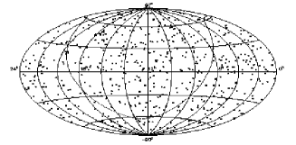
Figure 1: (left) The sky distribution of the 212 defining sources in the ICRF (from Ma et al. 1998 Fig. 10); (right) the sky distribution for all sources in the ICRF (from Ma et al. 1989, Fig. 13).

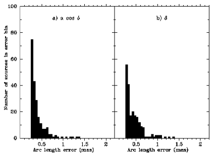
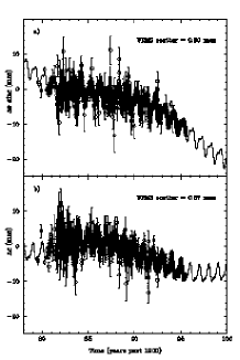
Figure 2: (left) The histogram of source position errors for the defining sources in $\alpha~{}$cos$\delta$ and $\delta$ (from Ma et al. 1998, Fig. 6a and 6b). (right) The measured nutation terms, with respect to the IAU 1980 model, observed for each session. The plotted curve is fit to the data using known nutation periods with 18 yr, 9 yr, 1 yr, 0.5 yr, and 14 days period (from Ma et al. 1998, Fig. 1a and 1b).

In the fall of 1995, a combined solution of all previous CDP observations determined thousands of parameters. The global parameters of the source positions and some telescope properties were held fixed over the whole set of data. The details concerning this complex least-squares fit to determine the most consistent set of source positions are given elsewhere (Ma et al. [1998]).

The resulting catalog contains three sets of sources. The ‘best’ 212 sources have frequent observations, relatively small position errors, and are dominated by a small-diameter radio component. They were used to define the orientation of the axes of the ICRF. In addition, there are about 300 sources with a smaller number of observations, less accurate positions, or obviously unstable positions (due to large source structure changes). About 100 sources with bright optical counterparts were included for potential frame-tie connections. The sky distribution of the defining 212 defining sources in the ICRF is shown in Fig. 1 (left). The distribution is relatively evenly spread north of the equator. The distribution for the entire set of ICRF sources is given in Fig. 1 (right). Observations are continuing and an additional 59 good quality sources have been added to the ICRF-extension1 catalog.

The distribution of the root-mean-square (RMS) radio source position error is given in Fig. 2 (left). In order to obtain realistic, but conservative error estimates, the internal errors, generated from the scatter among the sessions, were multiplied by 1.5 and then added in quadrature to a 0.25 mas error. These errors should then include structure effects over time and frequency. The accuracy of the ICRF realization of the ICRS axes is about 0.02 mas. An indication of the accuracy of the CDP observations can be seen in Fig. 2 (right) which shows the derived correction to the pole orientation (nutation) obtained for each 24-hour CDP session. It was fit to a realistic model known from geophysical and gravitational considerations with an RMS of the fit of about 0.3 mas. This is another indication of the accuracy of the frame realization for a 24-hour long session.

4.2 Frame Ties

Since the ICRF frame is accurate at the level of a few 0.02 mas and is stable over time scales of decades, it is advantageous to link other frames to it. The link to the FK5 frame was discussed in connection with continuity of the direction of the pole and origin of right ascension, with the ICRF adopting the FK5 pole at a specific epoch of time.

The Hipparcos catalog (Perryman et al. [1997]) contains observations between 1989.85 and 1993.21 of over 100,000 stars brighter than 12-mag. These observations were placed on the Hipparcos Reference Frame (Høg, E. et al. [1997]) to an accuracy of 1.0 mas. The link between the Hipparcos optical frame and the ICRF was accomplished in several ways. First, the few bright stars with significant radio emission were observed with the VLBI, the VLA and with Merlin in order to determine the radio positions with respect to the ICRF (Lestrade et al. [1995]). Accurate parallaxes and proper motions were also obtained for these radio emitting stars (Boboltz et al. [2003]). Secondly, comparison of the Hipparcos optical with HST observations linked these stars to extragalactic objects, and then to nearby ICRF objects which could be detected by HST. Next, additional optical observations using ground based telescopes also helped link Hipparcos positions to nearby galaxies. Finally, the earth orientation parameters were obtained from the Hipparcos observations and then compared with that obtained from that from nearly concurrent VLBI observations (Lindegren & Kovalevsky [1995]). With these comparisons, the Hipparcos optical catalog is now consistent with the ICRF to about 0.6 mas in position and 0.25 mas/yr for axis rotation. However, the position of an individual star and the reference frame tie decreases in accuracy with time because of the proper motion uncertainties of the stars of 1 mas per year.

The link of the ICRF to the planetary dynamic ephemeris was accomplished using several techniques. First, the time of arrival of a pulsar signal is sensitive to the orbital motion of the earth. By comparing the pulsar position derived from timing analysis with that obtained with VLBI observations, improvements in the dynamics of the earth motion could be obtained (Dewey et al. [1996]). Secondly, occultations of radio sources with solar system objects also tie the ICRF to that of the planetary ephemeris. Finally, radio interferometry of spacecraft with respect to nearby ICRF source also improved the frame tie between the two systems; for example, the observations the Magellan and Pioneer spacecraft with respect to nearby quasars (Folkner et al. [1993]). Comparison of the lunar ranging with VLBI earth orientation results were also important in tying the two frames together (Folkner et al. [1994]). The resulting JPL DE405 ephemeris is connected to the ICRF to about 1.0 mas in position and about 0.05 mas/yr in rotation (Standish [1998]), and the tie has recently been improved by a factor of two or three (Border 2003, private communication)

4.3 The Future of the ICRF

The ICRF will be the best realization of a quasi-inertial system at least until 2015 when the Space Interferometry Mission (SIM) has been in operation for several years. Hence, improvements in the ICRS and the accuracy of the ICRF positions are needed, and may be obtained in several ways. First, many more observations of the ICRF sources have been made since the original solution was made in 1997, and improved positions are designated as the ICRF-ext1 catalog. A further update, ICRF-ext2, is expected (Fey et al. 2004, in preparation). Secondly, VLBA observations, in its search for suitable calibrators needed for phase referencing (Beasley et al. [2002]; Fomalont et al. [2003]), have produced a catalog of over 2000 radio sources, some of which are candidates for additions to the ICRF catalog. Also, the number of experiments for sources in the southern hemisphere (Roopesh et al. [2003]) has enlarged over the last ten years. A new defining list of ICRF sources may be generated in the next five years, with an expected improvement in the grid accuracy of about a factor of two. However, discontinuities between the old and new frame definitions must be avoided.

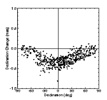
Figure 3: (left) The difference in the declination of the ICRF sources, as a function of declination, using global solutions with and without a tropospheric gradient in the modeling (from Ma et al. 1998, Fig. 4). (right) The change of position of three ICRF sources as a function of time caused by moving emission substructure near the radio core (from Ma et al. 1998, Fig. 2). The abscissa scale covers eight years and 1 mas is indicated in the middle plot.

A major source of error in the parameters associated with the ICRF is caused by the variable tropospheric delay; it is the major contributor to the current limit of 0.25 mas accuracy for the good quality sources. Although the troposphere zenith path-delay and gradient are modeled every hour during most 24-hour sessions, the structure and kinematics of the troposphere are extremely complicated, and the typical RMS delay scatter, after obtaining the best solution, is about 25 psec at a 5000-km baseline, which corresponds to a positional error of about 0.2 mas at 8 GHz. More sophisticated models, better monitoring of the tropospheric delay using GPS satellites, and ground measurements of water vapor emission in the line of sight to a source could decrease this uncertainty to one-half of the present level, but progress has been slow. An example of the gain in precision by an improvement in the tropospheric modeling is shown in Fig. 3 (left). The plot shows the difference in the derived declination of sources between two reductions of all of the 24-hour sessions in 1995: one reduction used an azimuthally-symmetric tropospheric delay model over each telescope and the other included a tropospheric gradient term (which is now routinely used). The differences as a function of source declination are up to 0.4 mas and show that systematic errors would have been present in the ICRF frame if the simpler tropospheric model had been used. Any remaining systematic error could be as large as 0.1 mas.

Another source of error is associated with the evolution of quasars—their changing structure. While these distant objects are fixed in the sky, the radio emission does not emanate from the galactic nucleus, but from the inner jet region which may be located 0.1 mas from the core at 8 GHz, and could be somewhat variable in position. Another source of error is caused by radio-emitting clouds of magnetic plasma which propagate down the jet and are often much brighter than the radio core nearer the galaxy nucleus. Fig. 3 (right) shows the apparent position versus time for several quasars which have undergone such evolution. The typical time-scale of changes are several months to years, and apparent position movements of 0.1 mas are common, and occasional changes as large as 1 mas can occur. With our knowledge of the nature of quasar radio emission, and with frequent monitoring of the radio source emission structure, it should be possible to model these evolutionary changes to remove the effects of these apparent positional changes (Fey & Charlot [1997]; Sovers et al. [2002])).

Finally, the ICRF positions are based on radio source properties at 8.4 GHz, but observations and studies are now underway to define a complementary ICRF at a frequency of 32 GHz (Lanyi et al. [2003]). At this higher frequency, the ionospheric refraction is smaller and the radio source structures are more compact. However, radio variability and structure changes will still be a problem. NASA-JPL plans to use 32 GHz for spacecraft telemetry, beginning in 2005. With an ICRF defined at this frequency, the tie between the planetary ephemerides and the quasar reference reference could be strengthened. However, such a tie is now perturbed by the limited modeling of the asteroids at the level of 0.2 mas per year which may be the dominant error (Standish & Fienga [2002]).

The advances in absolute astrometric measurements over the next 20 years (including space interferometry) may reach accuracies at the level of 0.01 mas, when a true space-time reference frame must be considered. This means that the astrometric system must become four-dimensionally based rather than the current system which is three dimensional, but with correction factors associated with the variable gravitational field of the solar system. Also, there is some discussion that the origin of the ICRF should be moved to the barycenter of the earth-moon system, rather than that of the solar system, because of the lower gravitation potential and diminished gravitational space distortion near the earth compared with that near the sun (Soffel et al. [2003]).

5 Relative Astrometry

Many astrophysical phenomena are associated with the accurate space motion of celestial objects, as well as their accurate position. For a source in the Milky way, the parallax is the only direct method of determining the distance, and its proper motion is often related to the evolution and formation of the object. From the orbital motion of a source, many properties of a binary or multiple system, including the detection of planet-like objects, can be made. For solar system objects the accuracy of radio interferometry is similar to that of lunar-laser ranging and range/Doppler measurements, and is complementary since interferometry determines positions on the celestial sphere and the other techniques determine the distance. Finally, the effect of the gravitational field in the solar system on the propagation of radio waves can be measured and compared with that predicted by GR or other theories of gravity.

5.1 Target-Calibrator Phase Referencing Methods

The determination of the motion of a radio source requires less complicated observations and reductions than that associated with all-sky ICRF observations. The reason is that the motion of a radio source can be obtained by measuring its position with respect to any detectable radio source, called a calibrator, that is fixed in the sky. If the calibrator-target separation in the sky is small and observations are switched rapidly between the calibrator and target, then the major error terms, shown in Eq. (1), are similar for the two sources and nearly cancel when their observed visibility phases are differed. This observation scheme is called phase referencing (Beasley & Conway [1995]).

From Eq. (1) the phase difference, $\triangle\phi^{s-c}_{l,m}$ at any time (t) between the target source $s$ and the calibrator $c$, for the baseline between telescopes $l$ and $m$ is

$$\triangle\phi^{s-c}_{l,m}(t)=\psi^{s}_{l,m}-\psi^{c}_{l,m}+\frac{\nu}{c}\Bigl{[}\big{(}{\bf R_{l}}-{\bf R_{m}}\big{)}{\bf\cdot}\big{(}{\triangle{\bf K}}^{s}(t)-{\triangle{\bf K}}^{c}(t)\big{)}$$

$$+\big{(}{\triangle}{\bf R}_{l}(t)-{\triangle}{\bf B_{m}(t)}\big{)}\cdot{\bf\delta K}^{s-c}+\partial^{2}\big{(}C_{l}(t)-C_{m}(t)\big{)}/\partial t^{2}$$

$$+\delta A^{s-c}(t)\big{]}+\frac{1}{\nu c}\delta I^{s-c}_{l,m}(t)$$ (2)

The first line shows the phases which dependent on the target and calibrator source structures and positions. The next two lines contains the differential delay errors. The small separation of the two sources, $\delta{\bf K^{s-c}}\equiv{\bf K^{s}-K^{c}}$, significantly decreases the effect of the telescope-location errors (in the most general sense), for example, by a factor of 50 for a one degree target-calibrator separation. Similarly, $\delta A^{s-c}\equiv A^{s}-A^{c}$ is the difference of the tropospheric delay error in the direction of the two sources, and $\delta I^{s-c}\equiv I^{s}-I^{c}$ is the ionospheric delay. The quasi-random short-term delays from small clouds will not cancel particularly well, even for close calibrators, but larger angular-scale deviations from the a priori model will cancel. This term will be discussed in more detail using multi-calibrator observations. Finally, the purely temporal (mostly clock) delay variations would cancel precisely if the calibrator and target were observed simultaneously. Otherwise, time-interpolation between calibrator observations is needed, and small second order clock errors will remain in the difference. The switching time between observations of the calibrator and target depend on temporal characteristics of the $C$ and $A$ terms in Eq. (5.1). The longest time for which interpolation between two observations will produce an accurate phase is called the coherence time, and varies from 30 sec at 23 GHz to 5 min at 1.4 GHz. During periods of inclement whether or strong ionospheric activity, the coherence time can decrease to 10 sec, making phase referencing impossible unless the calibrator and target are observed simultaneously.

5.2 Phase Versus Group Delay

The differential delay error between the calibrator and target are often less than 5 psec. Even at a high frequency of 23 GHz, the corresponding phase difference in $\triangle\phi^{s-c}_{l,m}(t)$ is less than one cycle and ambiguities of the phase are unlikely to occur. (Changes more than one cycle can be used as long as the phase between subsequent calibrator observations are connected properly.) The group delays can still be obtained by observing at several frequencies; however, this is not recommended, unless necessary, for several reasons. First, the precision of the visibility phase is greater than that of the group delay by the factor $\nu/\Delta\nu$ where $\nu$ is the observing frequency and $\Delta\nu$ is the spanned frequency range used to determine the group delay. For a reasonably strong sources, the typical delay error using the measured phase is $<1$ psec, while that for the group delay is about 10 psec. Since the all-sky observations, described for the CDP observations have typical residuals of 25 psec, which are dominated by the troposphere errors, the use of the much more accurate phase data (if it were possible to sort out cycle ambiguities) would not provide more accurate solutions than use of the group delay. On the other hand, the delay errors from a phase-referencing experiment are often $<5$ psec, which is less than the inherent group delay accuracy, but not the phase accuracy.

Another reason for using the phase, rather than the group delay, is to preserve the imaging capability afforded by the visibility phase. If the error terms in the second line of Eq. (5.1) can be determined (or assumed to be negligible), then Fourier imaging of the residual phase will produce an image of the source with its position relative to that of the calibrator. Even if the target source is extremely weak and cannot be detected during a single observation, such Fourier imaging of the entire target data set will produce an image from which accurate astrometric information can be obtained. For these weak sources, the group delay cannot be measured.

5.3 Calibrator Properties

The two most important properties of a calibrator source are its proximity in the sky to the target, and the strength of a compact radio component which must be detectable within a coherence time. In order for the calibrator phase to be accurately determined in a few minutes, the radio core must contain no less than  20 mJy (using the VLBA at 8 GHz at 64 MHz bandwidth which gives an RMS noise of 4 mJy). The use of a much stronger calibrator source which is more distant from the target than a fainter, but otherwise suitable calibrator, is not recommended. The decrease in the measurement phase error from a stronger source is more than balanced by the increase in differential errors between the calibrator and target.

Many calibrators contain very extended emission and even most compact radio cores are not true point sources. The phase effect of this structure is contained in the $\psi^{c}$ term in Eq. (5.1). Using the self-calibration techniques for which images of strong sources can be made (Cornwell & Fomalont [1999]), the structure phase can be obtained and removed. Thus, imaging of all calibrators should be done routinely.

A more serious problem is the variable position offset of the calibrator $\triangle{\bf K^{c}}(t)$ between observing sessions, since this change is translated directly into an apparent position change of the target. This problem is associated with extended sources where the maximum radio brightness or centroid brightness moves along the jet and with respect to the (fixed) galaxy nucleus (see Fig. 3 (right) for some examples). Even for compact sources, it is possible that its position shifts with time since the radio emission probably emanates from the inner part of the radio jet which may not be a stationary position with respect to the galaxy nucleus. When trying to reach astrometric levels $<0.1$ mas in a target over a period of time longer than a few months, it is crucial to image the calibrator in order to determine the probable angular change from the calibrator evolution.

Only a limited number of suitable calibrators are contained in the ICRF catalog. Over 2000 additional calibrators can be found in the VLBA surveys of calibrations (Beasley et al. [2002]; Fomalont et al. [2003]), and most have derived positions which are within 1 mas of the ICRF grid because they have been observed in one or more of the CDP 24-hour sessions. Independent searches for calibrator sources, which are near a desired target source, also can be undertaken using preliminary observations of km-sized arrays (VLA, WSRT, ATCA) to search for faint, compact flat-spectrum, candidate sources. At 1.4 GHz, the field of view of many VLBI arrays are sufficiently large so that a calibrator can usually be found sufficiently close to the desired target, and both can then be observed simultaneously.

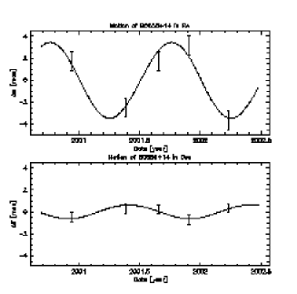
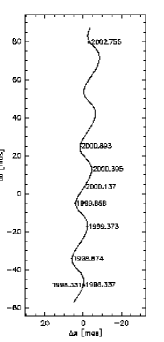
Figure 4: (left) The e/w and n/s parallactic motion of pulsar B0656+14 with respect to an in-beam calibrator $16^{\prime}$ away. The fit is shown by the curve. (right) The motion of pulsar B0950+08 using a calibrator that is $3^{\circ}$ away, but using a multi-frequency technique for removing the differential ionospheric refraction. The best fit proper motion and parallax are shown by the curve.

6 Relative Astrometric Results

In this section several phase-referencing astrometric experiments illustrate the techniques which are currently being used. The first example for B0656+14 illustrates a simple phase-referencing (in-beam) experiment. The second example for B0950+08 describes a scheme for removing ionospheric refraction using multi-frequency observations. The third example for HD8703 illustrates observations over many years to determine the orbital motion of a resolved radio source, and the problems associating with calibrator structure changes over time. All three of these examples assume that the phase error of the calibrator is a perfect measure of the phase errors of the target. The last example, the measurement of the deflection of a quasar by the jovian gravitational field, shows that by using more than one calibrator, relative positional accuracies less than 0.01 mas can be obtained from a six-hour observation.

6.1 Simple Phase Referencing

The pulsar PSR B0656+14 was observed with the VLBA at 1.67 GHz for five sessions, separated by about six months each, between epochs 2000.9 to 2002.5 (Briskin et al. [2003]). A calibrator, J0658+1410 with flux density 35 mJy, was found by preliminary VLA observations near the pulsar, only $16^{\prime}$ away, within the reception area of the VLBA antennas, so that both ‘in-beam’ calibrator and target were observed simultaneously. Because of the proximity of the calibrator and target, the differential delay errors were assumed to be zero. The calibrator image was sufficiently point-like; hence, its structure phase was assumed to be zero and its apparent position was assumed fixed in the sky since it is almost certainly an extra-galactic radio source. Images of the pulsar were then made from $\triangle\phi^{s-c}$ using the standard Fourier-techniques. The pulsar position was determined from the location of the peak of the pulsar image, with error estimates. Its peak flux density was 3.6 mJy and was far too weak to be detected in a single observation and to derive a group delay.

Using the images of the pulsar made from each session, the proper motion and parallax were accurately determined. The motion associated with the parallax motion (after removal of the proper motion) is shown in Fig. 4 (left). The parallax $\pi=3.47\pm 0.36$ mas, corresponding to a distance of $291\pm 30$ pc. The RMS of the fit for each epoch was about 0.6 mas which is impressive for a relatively weak radio source.

6.2 Ionosphere Removal

Another experiment, also a measurement of the motion of a pulsar, did not have the luxury of an available in-beam calibrator. Using the VLBA, alternating observations of the pulsar B0950+08 and calibrator J0946+1017, about $3^{\circ}$ away, were made every minute over a period of 7 hours, for 4 sessions between 1998.33 and 1999.85 (Briskin et al. [2000]). With the relatively large calibrator-target separation, the ionospheric refraction at 1.6 GHz was expected to be the dominant source of error. Since the pulsar is strong, about 64 mJy, the observations of the pulsar and calibrator were made at eight frequencies, simultaneously, between 1.31 GHz and 1.71 GHz. The differential phase error terms in Eq. (5.1) can then be written more generally as

$$\triangle\phi^{s-c}_{l,m}(t)=\frac{\nu}{c}\tau^{s-c}_{n}(t)+\frac{1}{\nu c}I^{s-c}(t)$$ (3)

where $\tau^{s-c}_{n}$ contains all of the non-dispersive delay terms (independent of frequency), and $I^{s-c}_{i}$ is the expected ionospheric delay component—between the two sources. By fitting the differential phase observed over the eight frequencies to a function of the form $A(t)\nu+B(t)\nu^{-1}$, both delay terms can be determine, and the ionospheric contribution removed from the observed differential phase. For telescopes more than 1000 km apart, the ionospheric-induced position shift can be as large as 10 mas per degree of source-calibrator separation, changing significantly within a time-scale of a few minutes; however a shift of 1 mas per degree over five to ten minutes of time is more typical for the source position jitter. Pulsar images, made from the phase before the ionosphere correction, were severely distorted.

The pulsar position was then obtained from the ionospheric-free images, and the position of B0950+08 determined in the same manner as for B0656+14. The structure phase of the calibrator J0946+1017 was determined at each observation epoch and removed from the differential phase. The calibrator appearance did not change significantly, hence it was assumed to be stationary in the sky. The derived motion of the pulsar is shown in Fig. 4 (right). The proper motion is $\mu_{\alpha}=-1.6\pm 0.4$ mas yr^-1, $\mu_{\delta}=29.5\pm 0.5$ mas yr^-1, and $\pi=3.6\pm 0.3$ mas.

6.3 Complex Motion and Calibrator Stability

The Gravity Probe B (GP-B) mission, developed by NASA and Stanford University, will fly four precision gyroscopes in earth orbit in order to measure two general relativistic precessions, a geodetic effect and a frame-dragging effect (Turneaure et al. [1989]). These precessions will be measured with respect to a suitably bright star whose position must be known to an accuracy of $<0.5$ mas. Thus, the goal of the associated radio observations was to find a suitable bright star with sufficient radio emission, and to determine its position and motion with the necessary accuracy. After exploratory observations, the RS Can Ven binary-star system, HR8703, was chosen. The radio emission comes from a main-sequence F-G star and the companions is a fainter K star with a known period of 24.65 days. This project illustrates some of the problems associated with both the target and the calibrator with variable source structure.

Figure 5: (left) The motion of HR8703 from phase referencing VLBI observations. The dashed line shows the best fit of the parallax and proper motion. (right) The dashed line shows the best fit orbit motion associated with the binary star HR8703 residual motion after removing the parallax and proper motion, shown on the left. The plotted crosses show the measured residual position, and the dots show the expected location on the orbit.

The radio position of HR8703 has now been measured from more than 20 observation sessions since early 1997, and is still continuing. The VLBA, the VLA and the three NASA Deep-space Network telescopes, at 8.4 GHz, had sufficient sensitivity that accurate group delays could be obtained for the star when it was stronger than 5 mJy, which was most of the time. The primary calibrator used was 3C454.3 (2251+158), about $1^{\circ}$ from the star. A second calibrator source, B2250+194, about $3^{\circ}$ away, was also used, as a control object to determine the accuracy of the observations. There are two groups performing the data reduction. One group is using the differential phase between HR8703 and 3C454.3, and the preliminary result reported here is from this group (Ransom ([2003]). Another group is analyzing the experiment using the group delay.

Using phase-referencing of HD8703 with 3C454.3 as the calibrator, good quality images of the binary system were made for each session. For some of the sessions, the radio emission showed two radio components separated by 1 mas, in some cases only one component was observed determined. The best fit to the parallax and proper motion (Fig. 5 (left)), was obtained by using the peak position of the radio emission when one component was detected, and using the geometric center when two components were detected. (This interpretation is consistent with the radio emission mechanism of fron RS Can Ven stars.) Also, the residual motion of the star, after removing the parallax and proper motion fit, showed a repeating pattern of 24.65 day period and, hence, this motion was associated with the binary orbit of the radio emission (Fig. 5 (right). The estimated error for the proper motion, parallax and orbital elements is about 0.1 mas.

The positions of HD8703 are with respect to that of 3C454.3. However comparison of the relative positions of 3C454.3 (see Fig. 4 (right, bottom)) and B2250+194 over the experiment period show relative motion between them in the order of 0.3 mas with a time scale of one year. Since both calibrators have extended, evolving structure, it is difficult to determine which source contributes to the apparent motion, and some of this shift may appear in the positions derived for HD8703. Taken over the five years of observations, these position errors lead to an proper motion uncertainty of $\sim 0.1$ mas yr^-1, which is still within the limited needed for GP-B mission. However, a more detailed analysis of the calibrator changes and other phase error terms in Eq. (5.1) is currently underway.

6.4 Multi-source Calibration Schemes and the Jupiter Deflection Experiment

On September 8, 2002 when Jupiter passed within $3.7^{\prime}$ of a background quasar J0842+1835, its gravitational field produced an apparent change (deflection) in the position of the quasar. At closest approach, according to GR, the deflection has two major components: a radial deflection of 1.19 mas, and a smaller deflection in the direction of motion of Jupiter of 0.051 mas. This smaller deflection component is caused by the gravitational aberrational produced by the relative motion of Jupiter and the earth, and is related to the speed of propagation of gravity (Kopeikin [2001]; Frittelli [2003]). Thus, by measuring this aberrational component to an accuracy less than 0.01 mas, an estimate of the speed of gravity could be obtained. However, this precision was about a factor of three to five better than had been previously obtained (see previous experiments as good examples). Such a gain in positional accuracy could only be obtained by determining the phase error terms associated with Eq. (5.1) more accurately.

Figure 6: (left) The Experimental Configuration for the Jupiter Bending Experiment: The observation periods are shown by the heavy portion of the Jupiter path, and the position of the three sources are nearly colinear. (right) The measured phase of the three sources on 2003 September 9 for the baseline between Mauna Kea, HI and Owens Valley, CA. Each source point corresponds to one minute of data, with a point observed every 4.5 min. The systematic phase difference between the sources after UT=17h is clearly shown. The phases separate with the source J0839, J0842 and J0854 phases with descending phase at any time. The differences are consistent with a phase gradient in the sky covering the three sources.

Although phase referencing between a calibrator and target removes much of the temporal dependence of the phase error, any coherent angular dependence in the sky will produce systematic phase errors between the target and calibrator, and produce distorted images and systematic errors in the position of the peak of the emission. This error can be diminished by choosing a calibrator closer to the target (if you can find one), or by using more than one calibrator to determine the angular dependence of the phase error. Preliminary VLBA test observations in 2001 suggested that such a multi-calibrator scheme was effective. Additional details on multi-source calibrations are given by Fomalont ([2003]).

The design of the Jupiter deflection experiment is shown in Fig. 6 (left). The observations were made at 8.4 GHz with the VLBA and Effelsberg, Germany telescope. In order to determine the phase errors toward the target source J0842, two calibrators, J0839 and J0854 on opposite sides of the target, were observed. Each source was observed for 1.5 min in turn, and the trio of scans were repeated every 4.5 min for ten hours over the day. Although the deflection of J0842 was strongest on 2002 September 8, identical observations on five days (September 4, 7, 8, 9, 12) were made in order to obtain sufficient redundancy to estimate realistic positional errors of the deflection. More details concerning the design and analysis of this experiment are given by Fomalont & Kopeikin ([2003]).

Fig. 6 (right, top) shows the measured phase for each of the three sources for a typical observing day and baseline. The overall temporal behavior of the phases, dominated by the clock and gross troposphere delay errors, are similar for the three sources. However, after UT=17h the phases for the three sources show displacements which are consistent with a simple phase gradient error covering the three sources: the displacement for J0839 from J0842 is in the opposite sense and about 25% of that between J0854 and J0842, as expected from their relative positions in the sky. Thus, the interpolation of the phase of J0839 and J0854 (weighted by their inverse distance from J0842) gives a very good estimate of the phase associated with J0842.

The corrected phase of J0842, $\Phi^{J0842}$, after the two source calibration, is shown in Fig. 6 (right, bottom). The phase scatter is small with a RMS less than 0.05 cycle, or about 0.040 mas. The slight offset from zero phase is associated with the sum of the position offsets from the a priori values, as seen in the expression for $\Phi^{J0842}$,

$$\Phi^{J0842}(t)=\phi^{J0842}(t)-0.80~{}\phi^{J0842}(t)-0.20~{}\phi^{J0854}(t)$$ (4)

$$=\psi^{J0842}+\frac{\nu}{c}\Bigl{[}\big{(}{\bf R_{l}}-{\bf R_{m}}\big{)}{\bf\cdot}\big{(}\triangle{\bf K}(t)^{J0842}-0.8~{}\triangle{\bf K}^{J0839}-0.2~{}\triangle{\bf K}^{J0854}\Bigr{]}$$

$$+\hbox{Terms of 2${}^{nd}$ order in time and angle}$$

where the 0.80 and 0.20 are the calibrator weighting factors for this particular configuration.

The position of the J0842 can be obtained by Fourier inversion of the corrected phase and measured visibility amplitude, or by a least-square fit of the phases if the source is sufficiently strong. The resultant displacement of the radio from the image center is a measure of the linear combination of offset positions (from the a priori positions), shown in Eq. (4). Assuming that the calibrator positions have not varied, any changes in the target position with time reflect a change in the target position.

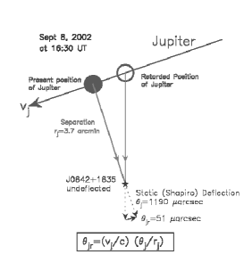
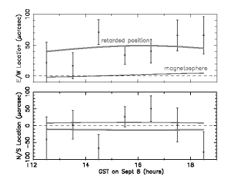
Figure 7: (left) The deflection of the quasar position from Jupiter is directed from the retarded position of Jupiter. The retarded deflection predicted by GR is 0.051 mas in the direction of Jupiter’s motion. (right) The measured relative position of the quasar on 2002 September 8 minus the measured relative position observed on the other four observing days. The position change on September 8 predicted by GR is shown by the curve labeled the retarded position. An estimate of the deflection caused by the Jovian magnetosphere is also labeled.

The goal of the September 2002 observation was to determine the speed of propagation of gravity, $c_{g}$, from the determination of the aberrational part of the quasar deflection, as outlined in Fig. 7 (left). For $c_{g}=c$, the expected deflection in the direction of Jupiter’s motion is 0.051 mas at closest approach. More generally, the deflection is proportional to $c_{g}^{-1}$. A graphical display of the experimental determination of this deflection term is given in Fig. 7 (right) which shows the measured position of J0842 every hour on September 8, relative to the other four observing days. These positions were determined from images of the residual phases and the observed visibility amplitudes. The measured aberrational deflection, averaged over September 8, was $0.050\pm 0.009$ mas, which gives a deflection that is $0.98\pm 0.19$ times that predicted by GR. The error estimates are consistent with the position of the target on the four off-Jupiter days when no change of position is expected. When converted into the speed of propagation of gravity, the result is $c_{g}=(1.06\pm 0.21)$c. A similar analysis on the data using only one calibrator, J0839, gave a positional error of 0.027 mas compared with 0.009 mas achieved using a second calibrator.

7 Summary

After a discussion of inertial frames and reference systems, the methods for determining the position of radio sources were discussed. First, all-sky observations used for the ICRF were used to determine absolute positions of radio sources which formed the definition of the celestial inertial reference system now in use. Secondly, phase referencing was described using four different experiments to illustrate several aspects of measuring the motion of radio sources to accuracies approaching 0.010 mas per session.

8 Appendix: The Speed of Gravity Controversy

Although the experimental result is not in doubt, there is disagreement over the correct role of gravity in this experiment. Kopeikin ([2001]), using the Einstein equations directly, interprets the retarded deflection component as a measure of the speed of propagation of gravity (see also Kopeikin & Fomalont ([2004])). Will ([2003]) concludes, however, that the retarded deflection component is associated with the aberration of light, not of gravity. Other interpretations are given by Asada ([2002]) and Samuel ([2003]).

At the Jenam2003 meeting in Budapest, a lively give-and-take session took place during the late afternoon of August 28. There were about 20-30 participants. The main points of view were presented by G. Schäfer (Institute for Theoretical Physics, Friedrich Schiller University, Jena, Germany), Sergei Kopeikin (University of Missouri-Columbia, MO, USA), and Gabor Lanyi (Jet Propulsion Laboratories, Pasadena, CA, USA)

Schäfer supported the point of view of Asada and Will that the experiment measured the speed of radio waves used in observations. The main arguments were:

1. gravity and light move along null geodesics and their speed can not be disentangle in the experiment;

2. the speed of gravity is associated with accelerated motion of light-ray deflecting bodies and thus, only with gravity waves;

3. the propagation of gravity effect shows up only in terms of order of $(v/c)^{4}$ in the metric tensor but the experiment is sensitive to $(v/c)^{3}$ terms only.

Kopeikin interpretation is that that the experiment measured the speed of propagation of gravity in the near zone of the solar system. In answer to Schäfer’s points, Kopeikin pointed out that:

1. The relativistic deflection of light by Jupiter depends on the Euclidean product of two null vectors at the point of observation—the vector of light propagation from the quasar and that of gravity propagation from Jupiter. Because the quasar and Jupiter are located at different positions on the sky, the gravity propagation direction can be separated from the light propagation direction and, thus, the speed of gravity could be measured.

2. There are different types of gravitational fields according to algebraic classification B. Y. Petrov. Only gravitational fields of type N (plane gravitational waves) are generated by the accelerated motion of bodies, and they exist only in the radiative zone of the solar system. Other types of gravitational fields are more general and can be associated with the velocity of the bodies. They dominate in the near zone of the solar system where the jovian deflection experiment has been done. Nevertheless, gravitational fields of the other Petrov’s types also propagate with finite speed which can be measured.

3. It is true that propagation of gravity effect shows up only in terms of order of $(v/c)^{4}$ in the metric tensor. But the metric tensor is not directly observable quantity in the jovian deflection experiment because it depends on specific choice of coordinates. Therefore, any reference to the metric tensor in connection with measured gravitational effects is irrelevant. What is observed is the phase of radio waves coming from the quasar which is perturbed by gravitational field of Jupiter from its retarded position, in accordance with Einstein’s equation predicting that gravity travels with finite speed equal numerically to the speed of light in vacuum. This relativistic effect of the retardation of gravity in the electromagnetic phase is gauge-independent and shows up already in terms of order of $(v/c)^{3}$ which we have observed.

9 Acknowledgments

The sections on reference frames and the ICRF were significantly improved from the suggestions and corrections by Chris Jacobs. I also thank Chopo Ma for his contributions, and Ryan Ranson for the preliminary HR8703 results.

References

- [2002] Asada, H. 2002, ApJ, 574, L69
- [2002] Beasley, A.J. et al. 2002, ApJS. 141
- [1995] Beasley, A.J. & Conway, J.E. 1995 in ASP Conf. Ser. 82, Very Long Baseline Interferometry and the VLBA, ed. J.A. Zensus, P.J. Diamond & P.J.Napier (San Francisco: ASP) 328
- [2003] Boboltz, D.A., Fey, A.L., Johnston, K.J., Claussen, M.J., deVegt, C., Zacharias, N. & Gaume, R.A. 2003, AJ, 126, 484
- [2000] Briskin, W.F., Benson, J.M., Beasley, A.J, Fomalont, E.B, Goss, W.M. & Thorsett, E. 2000, ApJ, 541
- [2003] Briskin, W.F., Thorsett, S.E., Golden, A. & Goss, W.M. 2003, ApJ 593
- [1999] Cornwell, T. & Fomalont, E. 1999, in Synthesis Imaging in Radio Astronomy, Asp Conf Series, 180, p187
- [1996] Dewey, R., Ojeda, M.R., Gwinn, C.R., Jones, D.L. & Davis, M.M. 1996, AJ, 111, 315
- [1998] Feissel, M & Mignard, F. 1998, A&A, L33
- [1996] Ferraz-Mello et al.1996, Dynamics, Ephemerides and Astronomy of the Solar System, IAU Symposium No. 172
- [1997] Fey, A.L. & Charlot, P. 1997, ApJS, 111, 95
- [1993] Folkner, W.M., Border, J.S., Nandi, S. & Zukor, K.S. 1993, Telec. & Data Acq Prog Report, TDAPR42-113, 22.
- [1994] Folkner, W.M., Charlot, P., Finger, M.H., Williams, J.G., Sovers, O.J., Newhall, X. & Standish, E.M. 1994, A&A 287, 279
- [2003] Fomalont, E.B, Petrov, L, MacMillan, D.S., Gordon, D. & Ma, C. 2003, AJ, 126, 2562
- [2003] Fomalont, E.B. & Kopeikin, S.M. 2003, ApJ, 598, 704
- [2003] Fomalont, E.B. 2003, in Future Directions in High Resolution Astronomy: A Celebration of the 10th Anniversary of the VLBA, in press.
- [1963] Fricke, W. et al. 1967 Veroff. Astron. Rechen-Inst. 10, Heidelberg
- [1988] Fricke, W.M., Schwan, H. & Lederle, T. 1988, Fifth Fundamental catalogue, Part I. Veroff. Astron. Rechen Inst. 32, Heidelberg.
- [2003] Frittelli, S. 2003, MNRAS, 344, L87
- [1971] Hazard, C., Sutton, J., Argue, A.N., Kenworthy, C.N., Morrison, L.V. & Murray C.A. 1971, Science, 233, 89.
- [1997] Høg, E. et al. 1997, A&A, 323, L57
- [2003] Honma, M et al. 2003, PASJ, 55, 57
- [1999] Johnston, K. J. & de Vegt, Chr. 1999, ARA&A, 37, 97
- [2001] Kopeikin, S.M. 2001, ApJ, 5556, L1
- [2004] Kopeikin, S.M., & Fomalont, E.B. 2004, submitted to Phys, Rev D.. Astro-ph/0311063
- [1938] Kopff, A. 1938, Abh. Preuss. Akad. Wiss. Phys.-Math, Kl, No 3
- [1995] Kovalenko, J. & Feissel, M. IAU Symposium No. 172, 455, Kluwer Academic Publishers (Dordrecht)
- [2003] Lanyi, G., Boboltz, D., Charlot, P., Fey, A., Fomalont, E., Gordon, G., Jacobs, C., MA, C., Naudet C., Sovers, O. & Zhang, L., 2003, this publication.
- [1995] Lestrade, J.-F. et al. 1995, A&A, 304, 182
- [1995] Lindegren, L. & Kovalevsky, J. 1995, A&A, 304, 189
- [1998] Ma, C., Arias, E.F., Eubanks, T.M., Fey, A.L., Gontier, A.-M., Jacobs, C.S., Sovers, O.J., Archinal, B.A. & Charlot, P. 1998, AJ, 116, 546.
- [1997] MacMillan, D.S. & Ma, C. 1997, Geo. Res. Let., 24, 453
- [1996] Niell, A. 1996 JGR, 101, 3227
- [1997] Perryman, M.A.C. et al. 1997, A&A, 323, L49
- [2003] Ransom, R.R. 2003, Ph.D. Thesis, York University, Canada
- [1970] Rogers, A.E.E. 1970, Radio Sci, 5, 1289
- [2003] Roopesh, O., Fey, A.L., Jauncey, D.L., Johnston, K.J., Reynolds, J.E. & Tzioumis, A.K 2003, Quasar Cores and Jets, 25th meeting of the IAU joint discussion 18
- [1993] Ryan, J.W., Clark, T.A., Ma, C., Gordon, D., Capretee, D. & Himwich, W.E. 1993, in Contributions of Space Geodesy to Geodynamics: Earth Dynamics, ed D.E. Smith & D. L. Turcotte (Washington:Am.Geophys. Unions), 37
- [2003] Samuel, S. 2003, Phys. Rev. Lett., 90, 231, 101
- [2003] Soffel, M. et al., 2003, AJ, in press.
- [2002] Sovers, O.J., Charlot, P, Fey, A.L., & Gordon, D. 2002, Paper presented at the IVS General Meeting, Tsukuba, Japan, Feb 2002. (http://ivscc.gsfc.nasa.gov/publications/gm2002/sovers/)
- [1998] Sovers, O.J., Fanslow, J.L. & Jacobs, C.S. 1998, Rev Mod Phys, 70, 1393
- [1998] Standish, E.M. JPL Planetary and Lunar ephemerides, DE405/LE405, JPL IOM 314.10-127
- [1989] Standish, E.M. 1990 A&A, 233, 252
- [2002] Standish, E.M. & Fienga, A. 2002, A&A, 384, 322
- [1994] Thompson, A.R., Moran, J.M. & Swenson, Jr., G.W. 1994, Interferometry and Synthesis in Radio Astronomy, 2nd edition, Wiley & sons, New York
- [1991] Treuhaft, R.N. & Lowe, S.T. 1991, AJ, 102, 1879
- [19887] Treuhaft, R.N. & Lanyi, G. 1987, Science 22, 251
- [1989] Turneaure, J.P., Everitt, C.W.F. & Parkinson, B.W. 1986, In Proceedings of the Fourth Marcel Grossmann Meeting on General Relativity, pp 411. Elseview Science Publishing.
- [1970] Wade, C.M. 1970, ApJ, 162, 381
- [2003] Will, C.M. 2003, ApJ, 590, 683