The Detection of Terrestrial Planets via Gravitational Microlensing: Space vs. Ground-based Surveys

Abstract

I compare an aggressive ground-based gravitational microlensing survey for terrestrial planets to a space-based survey. The Ground-based survey assumes a global network of very wide field-of-view $\sim 2$m telescopes that monitor fields in the central Galactic bulge. I find that such a space-based survey is $\sim 100$ times more effective at detecting terrestrial planets in Earth-like orbits. The poor sensitivity of the ground-based surveys to low-mass planets is primarily due to the fact that the main sequence source stars are unresolved in ground-based images of the Galactic bulge. This gives rise to systematic photometry errors that preclude the detection of most of the planetary light curve deviations for low mass planets.

University of Notre Dame, Notre Dame, IN 46556, USA

1. Introduction

Gravitational microlensing can be used to detect extra-solar planets orbiting distant stars (Mao & Paczyński 1991; Gould & Loeb 1992) with relatively large photometric signals as long as the angular planetary Einstein Ring radius is not much smaller than the angular size of the source star (Bennett & Rhie 1996). For giant source stars in the Galactic bulge, however, the signals of Earth-mass planets are largely washed out by their large angular size, but Galactic bulge main sequence stars are small enough to allow the detection of planets with masses as low as $0.1M_{\oplus}$.

This fact has led to suggestions that ground-based microlensing surveys might be able to measure the abundance of Earth-like planets (Tytler 1996; Sackett 1997). However, the initial estimates of the sensitivity of such a survey neglected the blending of main sequence source stars in the bulge that is illustrated in Fig. 1. The brightness of the source stars was over-estimated, and it was not realized that the actual source stars were blended with several other stars of similar brightness in ground-based images. More realistic estimates of the sensitivity of the proposed ground-based extra-solar planet searches indicated very poor sensitivity to terrestrial planets (Peale 2003), and suggested that only a space-based survey (Bennett & Rhie 2002) could discover a significant number of Earth-like planets.

In this paper, we simulate the most capable ground-based microlensing survey that could reasonably be attempted: a network of three 2-m class wide field-of-view telescopes spanning the Globe in the Southern Hemisphere that are dedicated to the microlensing planet search survey for four years.

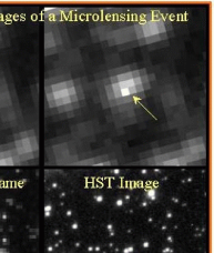
Figure 1.: The difference between ground and space-based data for microlensing of a bulge main sequence star is illustrated with images of microlensing event MACHO-96-BLG-5. The two top panels are 50 min. R-band exposures with the CTIO 0.9m telescope taken in 1” seeing at different microlensing magnifications, and the two images on the bottom have been constructed from HST frames. Ground-based photometry suggests that the lensed source star is bulge “turn-off” star 1-2 magnitudes brighter than the top of the bulge main sequence, but the HST image reveals that the actual source star is bulge G-dwarf on the main sequence.

2. Simulation Details and Results

Many of the details of our simulations have been described in Bennett & Rhie (2002), but there are additional details that must be added to describe the observing conditions at ground-based observatories. I assume that the microlensing survey telescopes are located at the best existing observatory sites in Chile (Paranal), South Africa (Sutherland), and Australia (Siding Springs). For Paranal, actual seeing and cloud cover records are available from the ESO web site. The Sutherland site in South Africa has conditions similar to La Silla in Chile (Peter Martinez, private communication), so the ESO records for La Silla (offset by 1 year) were used as a proxy for Sutherland. Standard airmass and wavelength correction formulae (Walker 1987) were used to convert the ESO seeing data to seeing estimates for bulge observations in the I-band, and the sky brightness was calculated following Krisciunas & Schaefer (1991).

For the observations from Australia, the 1997-1999 seeing records from the MACHO Project have been used since the Mt. Stromlo Observatory and Siding Springs have very similar seeing. To compensate for the optical effects of the MACHO telescope, 0.8” was subtracted in quadrature from all the MACHO telescope seeing values. The number of clear nights was adjusted slightly to meet the long term averages for each site as listed in Peale (2003).

An important input to this simulation is the systematic crowded field photometry errors that are assigned. The OGLE-III EWS data (Udalski 2003) provides a set of photometry for stars with brightness varying in a predictable way (due to microlensing) using the most accurate crowded field photometry method devised to date (Alard & Lupton 1996). By fitting to point-source, single-lens light curves to the 2002 OGLE-III EWS data for stars brighter than $I<17$, we find an assumed systematic error of 0.7% of the total flux at the PSF peak of each star seems to give fit $\chi^{2}\simeq 1$. The systematic errors appear to be larger for fainter stars or for other data sets, but I adopt this as a systematic error estimation formula.

This systematic error implies a limit to the useful size of a microlensing planet search survey telescope. Once the systematic error dominates, it is no longer useful to go to a larger telescope. Our simulation results yield an optimal telescope aperture of about 2-m with a 6 sq. deg. field-of-view (FOV). Larger telescopes could detect some more planets by cycling between two or more fields, but the gain is not large because of the rapid decrease in the microlensing rate away from the central Galactic bulge.

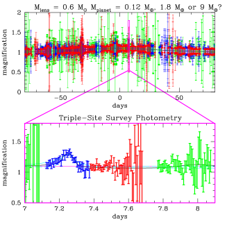
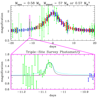
Figure 2.: Two example light curves from our ground based microlensing survey simulation, which allow the formal detection of the signal of a terrestrial. Data from Chile, South Africa, and Australia are shown represented by red, blue, and green error bars, respectively. The black and cyan light curves represent different microlensing models, and the magenta curve is the best fit non-planetary model. In both of these cases, the uncertainty in the planetary mass is more than two orders of magnitude. The source stars for these events have $I=21.1$ and $I=20.8$, respectively.

Fig. 2 shows an example of two light curves that would be considered planet detections by the criteria of Bennett & Rhie (2002) for a space-based survey (a $\Delta\chi^{2}>160$ improvement for the planetary lensing model over the best single lens model). But the uneven data quality due to seeing variations and cloud cover imply that the planetary parameters cannot be constrained. Thus, while the planetary signal is detectable for these events, terrestrial planets cannot be discovered with data like this. The situation is only slightly better for the events shown in Fig. 3, where the poor seeing in Australia, and low S/N of the planetary deviation conspire to prevent determinations of the planetary masses.

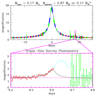
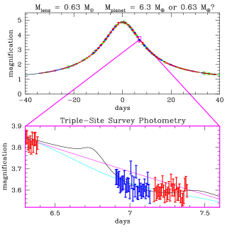
Figure 3.: Two additional simulated light curves for events with detected light curve deviations due to terrestrial planets where the light curve coverage or quality is not sufficient to determine the planetary mass. The source stars for these events have $I=22.0$ and $I=18.2$, respectively.

Of course, sometimes a planetary signal will be seen during good observing conditions, yielding light curves that can accurately determine the planetary parameters. This is the case for the two events shown in Fig. 4. Generally, such events have planetary deviations that occur at high magnification, such as the event on the left or have large amplitude deviations like the event on the right.

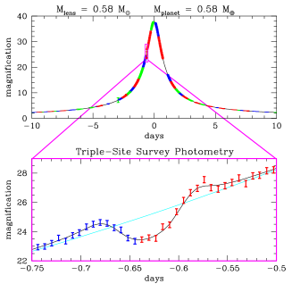
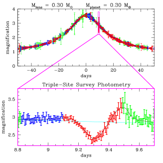
Figure 4.: Examples of light curves from our simulations where the light curve coverage and photometric accuracy allows for accurate determination of the terrestrial planetary parameters. These are both examples of simulated planetary discoveries. The source stars for these events have $I=20.5$ and $I=20.0$, respectively.

Intermediate between the poorly covered planetary detections shown in Figs. 2–3 and the well covered planetary discoveries shown in Figs. 4 are the light curves shown in Fig. 5. In both cases, the planetary parameters can be formally determined. However for the event on the left, the source star brightness is only $I=24.6$. If the photometry errors are not random, as is likely for systematic errors, then the brightness of the source star cannot be determined from the light curve fit. Hence, the planetary parameters will be poorly constrained. For the light curve on the right, the parameters can be determined despite the relatively poor coverage of the deviation because the deviation shape contains redundant information. However, the poor light curve coverage means that the redundancy cannot be used to confirm the interpretation of the event. This is a serious drawback because the planet discovery cannot be confirmed in any other way.

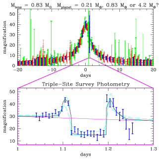
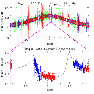
Figure 5.: Examples of simulated light curves with detected terrestrial planet signals, where the planetary parameters can formally be determined. The source stars for these events have $I=24.6$ and $I=19.3$, respectively.

It is clear from Figs. 2-4 it is sensible to consider two different categories of detected planetary events: “detected” planets and “discovered” planets. The “detected” category includes all planets with planetary signals that provide at least a $\Delta\chi^{2}\geq 160$ improvement over the best single lens fit. Clearly, the events shown in Fig. 4 should be in the “discovered” while those shown in Figs. 2 and 3 should not be in this category. We define the planet “discovered” category with the following criteria. Each planetary light curve deviation is split up into 1-3 separate deviation regions of positive or negative magnification with respect to the single lens curve with the same parameters. The first and last regions are considered be begin and end when the deviation reaches the with 10% of the maximum planetary deviation or 0.3% of single lens magnification. For a planet “discovery”, each the observations must cover at least 40% of each planetary deviation region, and at least 60% of each total deviation. All measurements are considered to contribute the light curve coverage unless their error estimates are larger than one third of the maximum planetary deviation. Also, because a significant component of the error estimates is a systematic error, we also require that each “discovery” light curve have at least one measurement that detected the stellar microlensing event by $\geq 10\sigma$ and one measurement that detects the planetary deviation by $\geq 5\sigma$. With these definitions, about one third of the detected planets pass the planet discovery threshold including both the events in Fig. 4 and the light curve on the left side of Fig. 5.

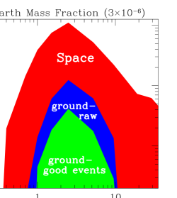
Figure 6.: The number of expected planetary detections as a function of orbital semi-major axis is compared for a space-based survey and a 3-site ground based survey. Planets with the Earth’s mass fraction of $\epsilon=3\times 10^{-6}$ are considered. The green region indicates the events detected from the ground that are well characterized, while the blue region indicates events which have a detectable signal which are not well characterized, as described in the text. The red region is the predicted sensitivity of the proposed GEST space mission according to the simulations of Bennett & Rhie (2002).

Fig. 6 compares the sensitivity of a 3-site network of 2m-class ground-based microlensing planet search telescopes vs. a space-based microlensing planet search telescope that would be appropriate for NASA’s Discovery Program (Bennett et al. 2003). At present, the cost cap for a Discovery mission is $360M, and the ground-based network that I have simulated would be roughly one fifth that cost, including all software development and operational expenses. The ground-based survey does the best at separations of 2–3 AU where the planet is near the Einstein Ring and is detectable in high magnification events. The ground-based survey would have about 30 times fewer planet discoveries and 10 times fewer raw detections of terrestrial planets at these separations. At 1 AU, the advantage of space for planet discoveries is a factor of 100.

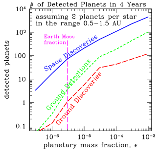
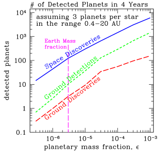
Figure 7.: The number of planet discoveries and detections as a function of the planetary mass fraction, $\epsilon$, is compared for a 3-site ground-based wide FOV telescope survey and a dedicated space mission. The left hand panel shows the comparison for planets in Earth-like orbits, while the right hand panel shows all planets.

The number of planet detections as a function of planetary mass fraction are shown in Fig. 7 for planets in Earth-like orbits and planets in all orbits. The left hand panel indicates that even if Earth-like planets in Earth-like orbits are quite abundant, the 3-site ground-based survey would only expect to find one with good light curve coverage.

The ground-based results in Fig. 7 are somewhat misleading for $\epsilon\geq 3\times 10^{-5}$ because these events can generally be detected with giant source stars, which have not been included in this simulation. These would add significantly to the ground-based detections, but would add little to the space-based detections. So, for planets with mass fractions about ten times that of the Earth, the ground-based survey may have an advantage.

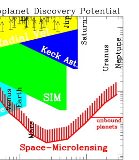
Figure 8.: The sensitivity of a space-based microlensing survey is plotted as a function of planetary mass fraction, $\epsilon$, and orbital semi-major axis. The yellow region gives the sensitivity of a 20-year radial velocity program on the Keck Telescope assuming a detection threshold of 10 m/sec, and the blue region indicates the sensitivity of a 10-year interferometric astrometry program with a 30$\,\mu$as detection threshold. The green and cyan regions indicate the sensitivities of the SIM and Kepler missions which are in development. The location of our Solar System’s planets and some of the extra-solar planets detected by radial velocities are shown. The horizontal lines indicate the sensitivity to free-floating planets since the more distant planets can sometimes be detected without seeing a microlensing signal from their star. Space-based microlensing clearly complements Kepler with its sensitivity to low-mass terrestrial planets at separations $\geq 0.7\,$AU.

3. Conclusions

I have carried out detailed simulations of the most capable ground-based microlensing terrestrial planet search program that could plausibly be attempted. The simulated survey employs three 2m class telescopes spanning the Globe in the Southern Hemisphere which observe the Galactic bulge whenever possible for a period of 4 years. Such a network is about 100 times less sensitive than a space-based survey which might only cost 5 times as much. So, without some dramatic improvement in ground-based crowded field photometry, it will not be possible to conduct a microlensing survey to determine the abundance of terrestrial planets in the inner Galaxy.

For a gravitational census of terrestrial planets, a space-based survey will be required (Bennett & Rhie 2002; Bennett et al. 2003). As Fig. 8 indicates, such a mission would complete the survey for terrestrial planets that will be started by the Kepler mission (Borucki et al. 2003) which is sensitive to Earth-like planets at separations $\mathrel{\hbox{\hbox to0.0pt{\hbox{\lower 4.0pt\hbox{$\sim$}}\hss}\hbox{$<$}}}1\,$AU using the transit method. A space-based microlensing survey would overlap Kepler with sensitivity at $\sim 1\,$AU, and extend sensitivity to terrestrial planets to all separations including free-floating planets, which may have been ejected from their parent stars during the planetary formation process.

References

- Alard & Lupton (1996) Alard, C., & Lupton, R. H., 1998, ApJ, 503, 325
- Albrow et al. (2001) Albrow, M. D., et al. 2001, ApJ, 556, L113
- Alcock et al. (2000) Alcock, C., et al. 2000, ApJ, 541, 734; (E) 557, 1035
- Bennett & Rhie (1996) Bennett, D. P., & Rhie, S. H., 1996, ApJ, 472, 660
- Bennett & Rhie (2002) Bennett, D. P. & Rhie, S. H., 2002, ApJ, 574, 985
- Bennett et al. (2003) Bennett, D. P., et al. 2003, SPIE, 4854, 141
- Borucki et al. (2003) Borucki, W. J., et al. 2003, SPIE, 4854, 129
- Gould & Loeb (1992) Gould, A., & Loeb, A. 1992, ApJ, 396, 104
- Krisciunas & Schaefer (1991) Krisciunas, C., & Schaefer, B. 1991, PASP, 103, 1033
- Mao & Paczyński (1991) Mao, S. & Paczyński , B. 1991, ApJ, 374, L37
- Peale (2003) Peale, S. J. 2003, AJ, 126, 1595
- Sackett (1997) Sackett, P. D., 1997, astro-ph/9709269
- Tytler (1996) Tytler, D. 1996, in “A Road Map for the Exploration of Neighboring Planetary Systems (ExNPS),” JPL Report, Chap. 7.
- Udalski (2003) Udalski, A., 2003, Acta Astronomica, 53, 291
- Walker (1987) Walker, G. 1987, “Astronomical Observations”, Cambridge University Press.