Uncorrelated Estimates of Dark Energy Evolution

Abstract

Type Ia supernova data have recently become strong enough to enable, for the first time, constraints on the time variation of the dark energy density and its equation of state. Most analyses, however, are using simple two or three-parameter descriptions of the dark energy evolution, since it is well known that allowing more degrees of freedom introduces serious degeneracies. Here we present a method to produce uncorrelated and nearly model-independent band power estimates of the equation of state of dark energy and its density as a function of redshift. We apply the method to recently compiled supernova data. Our results are consistent with the cosmological constant scenario, in agreement with other analyses that use traditional parameterizations, though we find marginal (2-$\sigma$) evidence for $w(z)<-1$ at $z<0.2$. In addition to easy interpretation, uncorrelated, localized band powers allow intuitive and powerful testing of the constancy of either the energy density or equation of state. While we have used relatively coarse redshift binning suitable for the current set of $\sim$ 150 supernovae, this approach should reach its full potential in the future, when applied to thousands of supernovae found from ground and space, combined with complementary information from other cosmological probes.

I Introduction

Recent measurements of the distance-redshift relation using type Ia supernovae (SNe Ia) Rieetal04 ; Baretal04 obtained using the Hubble Space Telescope further strengthened the evidence that the rate of expansion of the universe is increasing in time perlmutter-1999 . This accelerated expansion is ascribed to a mysterious component called dark energy that comprises about 70% of the energy density of the universe. In addition to supernova data, additional pieces of evidence come from the combined study of the large scale structure and the cosmic microwave background anisotropy measurements Tegetal03 . While the presence of dark energy is by now well established, we are at an early stage of studying and understanding this component. It is hoped that more accurate cosmological measurements will further constrain parameters describing dark energy and eventually shed light on the underlying physical mechanism.

Dark energy is most simply described by its present day energy density relative to the critical value, $\Omega_{DE}$, and its equation of state defined as the ratio of pressure to density, $w\equiv p_{DE}/\rho_{\rm DE}$ turner_white . In general, $w$ is allowed to freely vary with time (or redshift), as is $\rho_{DE}$. In practice, it is difficult to constrain $w(z)$ or, say, the scaled energy density $f(z)\equiv\rho_{DE}(z)/\rho_{DE}(0)$, when they are described by more than a few parameters due to severe parameter degeneracies entering the observable quantity (luminosity distance, in the case of SNe Ia). Even though it is in principle possible to recover the function $f(z)$ or $w(z)$ directly from supernova measurements Star98 , in practice one has to fit the noisy data with a smooth functional form HutTur01 which introduces error and bias (for a valiant attempt to do this with current data, see DalDjo04 ). Another general approach is to model $w$ or $f$ using a cubic spline in redshift (e.g. WanTeg04 ), but again the paucity of data limits the spline to a few points in redshift, while having more points would correlate the measurements making the interpretation somewhat difficult.

Constraints from the new SN Ia data Rieetal04 suggest that dark energy is consistent with the cosmological constant scenario Rieetal04 ; WanTeg04 , agreeing with previous work Alaetal03 ; WanFre04 . However, these (and other) analyses are typically based on particular models — either a linear variation with redshift CooHut99 or the evolution that asymptotes to a constant $w$ at high redshift Lin03 , or perhaps a more complicated parameterization CorCop02 — that are used to describe redshift variation of the dark energy equation of state. While these forms do a very good job in fitting $w(z)$ due to a variety of proposed mechanisms that could be responsible for dark energy Lin04 , one should keep in mind that we are far from having any solid leads as to what to expect for the dark energy evolution. Given the constant increase in the quality and quantity of SN Ia data, it is timely to consider whether one can use current data to derive model independent conclusions on the evolution of dark energy.

In this paper, we introduce a variant of the principal component analysis advocated in Ref. HutSta03 . We make use of the most recent type Ia supernova data from Ref. Rieetal04 and present a view of dark energy complementary to other approaches. At the same time, we are seeking to answer one of the most important questions at present: is dark energy consistent with the cosmological constant scenario or not? Our analysis is facilitated by the fact that our measurements are completely uncorrelated. Finally, we briefly comment on the applicability of this approach to future datasets. Throughout we assume a flat universe.

II Methodology

We would like to impose constraints on the parameters $p_{i}$ ($i=1\ldots N$) that describe the dark energy equation of state $w(z)$ or its energy density $f(z)$, each $p_{i}$ being suitably defined in the $i^{\rm th}$ redshift bin. In addition to these, we have two more parameters: matter density relative to the critical $\Omega_{M}=1-\Omega_{DE}$ and the Hubble constant $h\equiv H_{0}/$(100km/s/Mpc). We first marginalize the full $(N+2)$–dimensional likelihood over these two (for the priors and assumptions, see Sec. III), and project them onto the $p_{i}$ space. The covariance of the $N$ resulting parameters is

$${\bf C}\equiv\langle{\bf pp^{T}}\rangle-\langle{\bf p}\rangle\langle{\bf p}^{T}\rangle$$ (1)

where ${\bf p}$ is the vector of parameters $p_{i}$ and ${\bf p}^{T}$ its transpose. These parameters can now be rotated into a basis where they are diagonal by choosing an orthogonal matrix W so that it diagonalizes the Fisher matrix

$${\bf F}\equiv{\bf C}^{-1}={\bf W}^{T}{\bf\Lambda}{\bf W}$$ (2)

where ${\bf\Lambda}$ is diagonal. It is clear that the new parameters $q_{i}$, defined as ${\bf q}\equiv{\bf Wp}$, are uncorrelated, for they have the covariance matrix ${\bf\Lambda}^{-1}$. The $q_{i}$ are referred to as the principal components and the rows of ${\bf W}$ are the window functions (or weights) that define how the principal components are related to the $p_{i}$. We refer the reader to Huterer & Starkman HutSta03 for a discussion on the application of principal components to the dark energy equation of state.

Let us now define ${\bf\widetilde{W}}$ by absorbing the diagonal elements of ${\bf\Lambda}^{1/2}$ into the corresponding rows of ${\bf W}$, so that ${\bf\widetilde{W}}^{T}{\bf\widetilde{W}}={\bf F}$ . Then, as emphasized by Hamilton and Tegmark HamTeg00 in the context of matter power spectrum measurements, there are infinitely many choices for the matrix ${\bf\widetilde{W}}$, as for any orthogonal matrix ${\bf O}$, ${\bf O\widetilde{W}}$ is also a valid choice that makes the parameters $q_{i}$ uncorrelated. While the principal components, $q_{i}$, have several nice features — in particular, the best-determined $q_{i}$ are smoother and have support at lower redshift than the poorly determined ones — their corresponding window functions are oscillatory, making the intuitive interpretation of the components somewhat difficult.

Here we advocate another choice for the weight matrix ${\bf\widetilde{W}}$: the square root of the Fisher matrix, ${\bf\widetilde{W}}={\bf F}^{1/2}\equiv{\bf C}^{-1/2}$ HamTeg00 . This choice is interesting since the weights (rows of ${\bf\widetilde{W}}$) are almost everywhere positive, with very small negative contributions, and this has been recognized as a useful basis in which to represent measurements of the galaxy power spectrum from large-scale structure surveys teg_SDSS_3DPS . The matrix ${\bf\widetilde{W}}$ is computed by first diagonalizing the Fisher (inverse covariance) matrix, ${\bf F}={\bf O}^{T}{\bf\Lambda O}$, and then defining ${\bf\widetilde{W}}={\bf O}^{T}{\bf\Lambda^{1/2}O}$. We normalize ${\bf\widetilde{W}}$ so that its rows, the weights for $p_{i}$, sum to unity. With this choice, Eq. (1) shows that the covariance of the new parameters, ${\bf q}\equiv{\bf\widetilde{W}p}$, is

$$\langle\,(q_{i}-\langle q_{i}\rangle)\,(q_{j}-\langle q_{j}\rangle)\,\rangle={\delta_{ij}\over\displaystyle\sum_{a}(F^{1/2})_{ia}\sum_{b}(F^{1/2})_{jb}}\,,$$ (3)

and parameters $q_{i}$ are manifestly uncorrelated. Furthermore, their weights are mostly positive and are localized in redshift fairly well. We illustrate this in the next section using current supernova data.

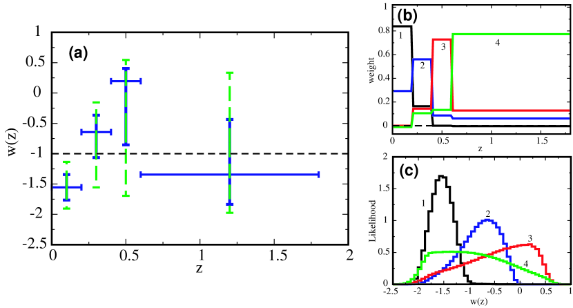
Figure 1: Uncorrelated band-power estimates of the equation of state $w(z)$ of dark energy are shown in panel (a). Vertical error bars show the 1 and 2-$\sigma$ error bars (the full likelihoods are shown in panel (c)), while the horizontal error bars represent the approximate range over which each measurement applies. The full window functions in redshift space for each of these measurements are shown in panel (b); they have small leakage outside of the original redshift divisions. The window functions and the likelihoods are labeled in order of increasing redshift of the band powers in panel (a). The window functions satisfy three of our requirements: they make the band-powers uncorrelated, they are fairly well localized in redshift, and they are almost everywhere positive. In panel (a), we have used a uniform prior of $0.22\leq\Omega_{M}\leq 0.38$ (a Gaussian prior $\Omega_{M}=0.3\pm 0.04$ gives very similar results), and we have assumed a flat universe throughout.

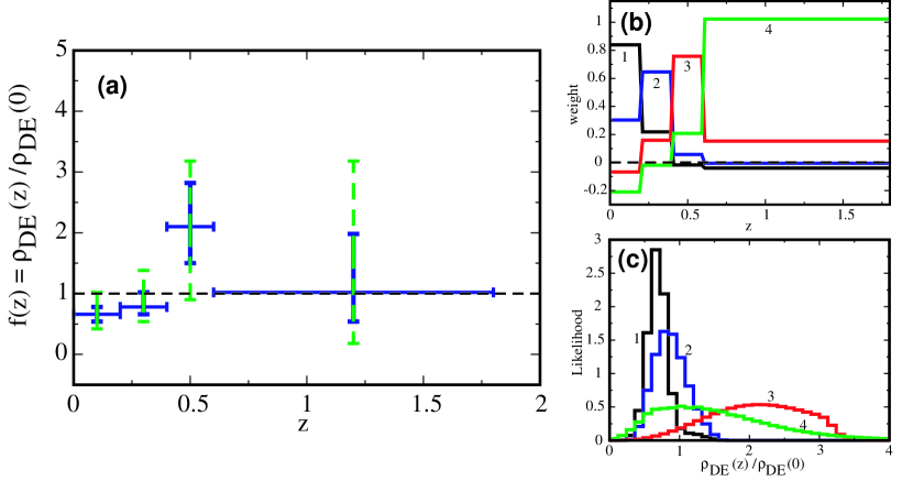
Figure 2: Same as Figure 1, but for $f(z)\equiv\rho_{\rm DE}(z)/\rho_{\rm DE}(0)$. Our band powers assume piecewise linear $f(z)$, with the exception of the band power corresponding to the largest-redshift bin, which assumes constant $f(z)$ across that bin.

III Results

We perform the analysis of the “gold” dataset from Riess et al. Rieetal04 . First, we need to parameterize $w(z)$ and $f(z)$ in redshift, thereby defining the parameters $p_{i}$ from Sec. II. We choose $w(z)$ to be piecewise constant in redshift and $f(z)$ to be piecewise linear (and continuous). These two assumptions are consistent, since the two functions are related as $w(z)=1/3\,(1+z)f^{\prime}(z)/f(z)-1$. Note that, in the limit of the large number of parameters $p_{i}$, the shape of the function across the redshift bin becomes irrelevant.

We choose $N=4$ bins with redshifts $0\leq z\leq 0.2$, $0.2\leq z\leq 0.4$, $0.4\leq z\leq 0.6$, $0.6\leq z\leq 1.8$, for both $w(z)$ and $f(z)$ constraints. While our choice of the number of parameters (or bins) is limited by the computing power required to perform the maximum likelihood analysis, we have repeated the same analysis with five parameters in each case and found consistent results. Future SN Ia data will lead to better constraints at all redshifts, requiring more parameters and perhaps the use of Markov chain Monte Carlo techniques, but for our purpose a simple analysis is sufficient. Furthermore, we have explored in detail the choice of the redshift binning, trying to strike a balance between band powers being narrow and having small error bars. Not surprisingly, we find that the constraints on $w(z)$ or $f(z)$ are much better at low redshift, and we put three of our four bins there, choosing their widths so as to get comparable constraints in each. We have varied the exact spacing of the bins, and found results consistent with the same underlying $w(z)$ or $f(z)$.

Finally, we describe the piecewise linear $f(z)$ as follows: we write $f(z)=1+g(z)$ (note that $g(z)=0$ corresponds to the cosmological constant scenario). We describe $g(z)$ by the sawtooth basis in redshift, where each tooth is $0.2$ wide and peaks in the middle of the corresponding bin. The highest-redshift bin presents a problem, since it is much wider than the others and implies that $f(z)$ may be forced to vary strongly across this bin. To prevent this, we make all basis vectors of the sawtooth 100% correlated in the highest redshift bin, essentially making $f(z)$ flat across this bin. We have checked that these details do not affect the results appreciably by repeating the analysis with a few alternative choices, and we believe that these assumptions are reasonable and intuitive.

The analysis is now straightforward: we compute the goodness-of-fit statistic $\chi^{2}$ for each model in the six-dimensional parameter space ($p_{1}\ldots p_{4},\Omega_{M},h$). We allow a generous range for the parameters $p_{i}$ (corresponding roughly to the vertical range in the left panels of the two Figures) and verify that changing the range leads to insignificant changes in the final constraints. We then marginalize the full likelihood over $\Omega_{M}$ and all values of $h$ and project it onto the $p_{1}\ldots p_{4}$ space. We use a flat prior $0.22\leq\Omega_{M}\leq 0.38$, corresponding to the $\pm 2\sigma$ allowed range from the joint analysis of various cosmological probes Tegetal03 . We have repeated our analysis with the Gaussian prior $\Omega_{M}=0.30\pm 0.04$ and found that the results are largely insensitive to the exact choice of either prior: the only notable change was that the first band power increases by about 0.15 with the Gaussian prior. The parameters $p_{i}$ are then rotated into the new parameters $q_{i}$, which are now uncorrelated, following the methodology described in Sec. II.

Figure 1 shows the final 68% and 95% CL constraints on the four band powers (i.e. the parameters $q_{i}$) representing $w(z)$. We also show the weights that describe going from correlated parameters $p_{i}$ to the uncorrelated $q_{i}$, as well as the full likelihoods of the four band powers. The horizontal error bars in the left panel show the extent of the original bins; although the components’ weights extend across the whole redshift range, the most weight ($\sim 60$% or more) is in these respective bins and the band powers are therefore sufficiently localized in order to be easily interpreted. Note also that the weights are mostly positive and have small negative contributions, as found in the context of matter power spectrum measurements HamTeg00 .

As shown in Fig. 1, the equation of state is consistent with $w=-1$ at the 95% CL in three out of four bins. We do find some ($>95\%$ CL) evidence that $w<-1$ at $z<0.2$; however, to confirm this result with certainty will require more data, and in particular more stringent control of the systematic errors. Nevertheless, it is interesting that we find a similar tendency in the data as seen in completely independent analyses that use different, and less general, parameterizations Alaetal03 ; Rieetal04 . The present approach, however, is less model dependent than these methods. In particular, any variations in the equation of state on redshift scales smoother than the binning scale can in principle be detected; more rapid oscillations cannot. This is why we consider this approach to be nearly model independent – it would be truly model independent if we used a large number of bins, as illustrated in Ref. HutSta03 .

We now consider another parameterization of dark energy – its energy density relative to the present value, $f(z)$. We repeat the analysis and obtain constraints on $f(z)$ shown in Fig. 2. They are roughly consistent with those for $w$, and are also consistent with the cosmological constant case at the 95% CL. Note that the likelihoods are fully contained in the allowed ranges, and we see no evidence for negative $f(z)$. The weights of $f$ are somewhat less well localized; however, the band powers are better determined than those of $w$, as expected from the fact that $f$ is related to the luminosity distance data through a single, and not double, integral relation.

IV Discussion and Summary

We have used a variant of the principal component technique to produce uncorrelated, nearly model independent estimates of the equation of state of dark energy $w(z)$ and its scaled energy density $f(z)$. We used four redshift bins in each case, and found results that are in good agreement with previous analyses. We further argued that the present approach nicely complements other methods that use conventional parameterizations of $w(z)$ and $f(z)$. Given that our band powers are uncorrelated, the interpretation of the cumulative evidence is particularly easy.

If dark energy is due to the cosmological constant, then $w=-1$ and $f(z)=1$, and all of our band powers should be consistent with those values, independently of their window functions. Conversely, if we ever find strong statistical evidence that even just one band power is different from $-1$ (for $w$) or $1$ (for $f$), we will have ruled out the cosmological constant scenario. While we do find a hint of such evidence in the first band power of $w(z)$, a definitive analysis will have to await more data and a careful assesssment of the systematics.

While we have presented an analysis with $\sim$ 150 supernovae and restricted ourselves to four bins in redshift, the generality and power of this method should make it perfectly suitable for the analysis of future supernova datasets, when the error bars are expected to improve by up to an order of magnitude and enable a much more quantitative analysis and comparison with models. Furthermore, the same techniques can be applied to a variety of other cosmological probes, as one can expect that their complementarity will considerably strengthen the SN Ia results. Finally, one can customize the proposed technique specifically to maximize the return of any given test (say, whether $w(z)=-1$ or not). With an increase in the number of type Ia supernovae at high redshift, it is likely that these interesting possibilities will be considered in the future.

Acknowledgments: We thank Eric Linder for useful comments on the manuscript. This work has been supported by the DOE at Case Western Reserve University (DH) and the Sherman Fairchild foundation and DOE DE-FG 03-92-ER40701 at Caltech (AC).

References

- (1) A. G. Riess et al., arXiv:astro-ph/0402512.
- (2) B. J. Barris et al., arXiv:astro-ph/0310843; R. A. Knop et al., arXiv:astro-ph/0309368; J. L. Tonry et al., Astrophys. J. 594, 1 (2003).
- (3) S. Perlmutter et al., Astrophys. J. 517, 565 (1999); A. Riess et al., Astron. J. 116, 1009 (1998).
- (4) M. Tegmark et al. [SDSS Collaboration], arXiv:astro-ph/0310723.
- (5) M. S. Turner and M. White, Phys. Rev. D, 56, R4439 (1997).
- (6) A.A. Starobinsky, JETP Lett. 68, 757 (1998); D. Huterer and M. Turner, Phys. Rev. D 60 081301 (1999); T. Nakamura and T. Chiba, Mon. Not. R. astron. Soc. 306, 696 (1999).
- (7) D. Huterer and M. Turner, Phys. Rev. D 64 123527 (2001); J. Weller and A. Albrecht, Phys. Rev. D 65, 103512 (2002); M. Tegmark, Phys. Rev. D 66, 103507 (2002)
- (8) R.A. Daly, S.G. Djorgovski, astro-ph/0403664
- (9) Y. Wang and M. Tegmark, arXiv:astro-ph/0403292.
- (10) U. Alam, V. Sahni, T. D. Saini and A. A. Starobinsky, arXiv:astro-ph/0311364; U. Alam, V. Sahni, and A. A. Starobinsky, arXiv:astro-ph/0403687.
- (11) Y. Wang and K. Freese, astro-ph/0402208.
- (12) A. R. Cooray and D. Huterer, Astrophys. J. 513, L95 (1999) [arXiv:astro-ph/9901097].
- (13) E.V. Linder, Phys. Rev. Lett. 90 091301 (2003).
- (14) P.S. Corasaniti and E.J. Copeland, Phys. Rev. D 65 043004 (2002); U. Alam et al., Mon. Not. Roy. Astron. Soc. 344, 1057 (2003).
- (15) E.V. Linder, Phys. Rev. D submitted (astro-ph/0402503).
- (16) D. Huterer and G. Starkman, Phys. Rev. Lett. 90, 031301 (2003).
- (17) A.J.S. Hamilton and M. Tegmark, MNRAS, 312, 285 (2000); M. Tegmark, Phys. Rev. D, 55, 5895 (1997).
- (18) M. Tegmark et al. [SDSS Collaboration], Astrophys. J., in press (astro-ph/0310725).