Radiative cooling, heating and thermal conduction in M87

Abstract

The crisis of the standard cooling flow model brought about by Chandra and XMM-Newton observations of galaxy clusters, has led to the development of several models which explore different heating processes in order to assess if they can quench the cooling flow. Among the most appealing mechanisms are thermal conduction and heating through buoyant gas deposited in the ICM by AGNs. We combine Virgo/M87 observations of three satellites (Chandra, XMM-Newton and Beppo-SAX) to inspect the dynamics of the ICM in the center of the cluster. Using the spectral deprojection technique, we derive the physical quantities describing the ICM and determine the extra-heating needed to balance the cooling flow assuming that thermal conduction operates at a fixed fraction of the Spitzer value. We assume that the extra-heating is due to buoyant gas and we fit the data using the model developed by Ruszkowski and Begelman (2002). We derive a scale radius for the model of $\sim 5$ kpc, which is comparable with the M87 AGN jet extension, and a required luminosity of the AGN of a $few\times 10^{42}{\rm erg\,s^{-1}}$, which is comparable to the observed AGN luminosity. We discuss a scenario where the buoyant bubbles are filled of relativistic particles and magnetic field responsible for the radio emission in M87. The AGN is supposed to be intermittent and to inject populations of buoyant bubbles through a succession of outbursts. We also study the X–ray cool component detected in the radio lobes and suggest that it is structured in blobs which are tied to the radio buoyant bubbles.

1 Introduction

The hot diffuse X-ray emitting gas (intracluster medium, ICM for short) provides a powerful tool to inspect the internal dynamics of galaxy clusters. For the typical density and temperature of the intracluster gas, the main emission mechanism is the bremsstrahlung and, for a large amount of clusters, the radiative cooling time in the central regions is significantly shorter than the Hubble time. As a consequence, if no additional heating mechanism is present, the gas cools and is expected to flow inwards, forming a cooling flow. The standard model of cooling flows (see Fabian, 1994, for a review) predicted the gas to be a multiphase medium in which there is a broad range of temperatures and densities present at all radii. Mass deposition rates were estimated to be as large as hundreds of solar masses per year (Allen et al., 2001). This model was strengthened by the general thought that in presence of magnetic fields the thermal conduction must be highly suppressed (Binney and Cowie, 1981; Fabian, 1994; Chandran and Cowley, 1998; Malyshkin, 2001), which is a necessary condition for the multiphase cooling to operate. In fact, no heating exchange between the different phases must occur in order that they may coexist. There is some observational evidence that modest magnetic fields are present throughout the intracluster medium. The current measurements of intracluster magnetic fields are based on Faraday rotation measure (RM) in radio sources seen through clusters (e.g. Kim, Kronberg and Tribble, 1991; Clarke, Kronberg and Böhringer, 2001; Feretti et al., 1999; Taylor et al., 2001); direct evidence also comes from measurements of extended regions of radio synchrotron emission in clusters (see e.g. Giovannini and Feretti, 2000; Fusco-Femiano et al., 2000; Owen, Morrison and Voges, 1999; Feretti, 1999). Both the excess RM values and the radio halo data suggest modest magnetic fields, at a few microgauss levels, throughout the cluster.

Recent XMM-Newton  and Chandra observations have shown that in the central regions, the temperature drops to about one third of its overall mean value and there is no evidence of temperatures smaller than $\sim 1-2$ keV (Peterson et al., 2001; Kaastra et al., 2001; Tamura et al., 2001; Allen et al., 2001), suggesting that the gas does not cool below these cutoff temperatures. Moreover, the new estimated mass deposition rates are significantly smaller than those evaluated by using previous X-ray satellites data (McNamara et al., 2001; Peterson et al., 2001). Lastly, the new data show that clusters spectra are better represented by a single (or double) temperature model rather than the standard multiphase (multi-temperature) cooling flow model (Molendi and Pizzolato, 2001; Böhringer et al., 2001; Fabian et al., 2001; Matsushita et al., 2002).

These new results clearly show that the standard cooling flow model is not a satisfying description of the internal dynamics of the ICM. Some source of heat which stops the cooling flow and balances radiative losses must be sought. The nature of this source and the origin of the heat mechanism is still unclear.

One possible candidate is thermal conduction. Recent works by Narayan and Medvedev (2001) and Gruzinov (2002) show that in the presence of turbulent magnetic fields, the conductivity can be as large as a fraction of the Spitzer value and thus can play a significant role in balancing cooling flows. As a consequence, thermal conduction has been recently re-introduced as a possible heat source to balance the energy losses (see e.g. Voigt et al., 2002; Voigt and Fabian, 2004; Fabian et al., 2002; Malyshkin, 2001; Zakamska and Narayan, 2003). However, as we will discuss more in detail in §5.1, thermal conduction fails in supplying the needed heat in the central regions (see also Voigt et al., 2002; Voigt and Fabian, 2004; Zakamska and Narayan, 2003).

Heating from a central active galactic nucleus is another possibility. The idea is supported by the fact that most of “cooling clusters” host a central active galactic nucleus with strong radio activity (Burns, 1990; Brighenti and Mathews, 2002). Several models in the literature explore AGN heating processes to assess if they can balance the radiative losses. One of the most appealing mechanisms involves buoyant gas bubbles, inflated by the AGN, that subsequently rise through the cluster ICM heating it up (Churazov et al., 2002; Böhringer et al., 2002; Brüggen and Kaiser, 2002a, b; Brüggen et al., 2002).

However, all the models predicting that radiative cooling is balanced only by energy input from the central AGN fail (McNamara, 2002; Zakamska and Narayan, 2003; Brighenti and Mathews, 2002). In particular, Brighenti and Mathews (2002) analyzed several heating mechanisms induced by the central AGN and concluded that no simple mechanism is able to quench the cooling flow. Moreover, the required mechanism needs a finely tuned heating source. Indeed, the heat source must provide sufficient energy to stop the cooling flow, but not enough to trigger strong convection or the metallicity gradients observed in all cooling flow clusters (De Grandi and Molendi, 2001) would be destroyed. As a consequence, an AGN can be an efficient mechanism in the very center of the cluster but it is unlikely to be strong enough to provide energy to the outer parts of the “cooling region”. So, it may be viewed as complementary to thermal conduction which fails in quenching the cooling flow in the innermost regions.

Recently, Ruszkowski and Begelman (2002) and Zakamska and Narayan (2003) concluded that both thermal conduction and heating from a central AGN can play an important role in balancing the cooling. In particular, Ruszkowski and Begelman (RB02 hereafter) developed a model where both thermal conduction and heating from a central AGN co-operate in balancing the radiative losses. One of the main advantages of this model is that it reaches a stable final equilibrium state and it is able to reproduce the main observed quantities, such as the temperature profile (with a minimum temperature $T\sim 1$ keV).

In this paper, we use M87/Virgo observations of three satellites (namely XMM-Newton, Chandra and Beppo-SAX) to test various heating models on this cluster. To this end, we apply to the M87 data the deprojection technique to recover some physical quantities of the ICM such as the gravitational mass, the entropy and the heating required to balance the cooling flow.

The paper is organized as follows: in §2 we report details about the analysis of the three (Chandra, XMM-Newton  and Beppo-SAX) M87 datasets; in §3, we revise briefly the spectral deprojection technique that we adopt for our analysis; in §4, we deproject the M87 data, we test that the spherical symmetry hypothesis holds and we derive the gravitational mass for M87; in §5, we determine the amount of extra-heating needed to balance the cooling flow when thermal conductivity is assumed to operate at a fraction of the Spitzer value. Lastly, in §6 we summarize our results.

2 Data analysis

Thanks to its proximity, the Virgo cluster and its giant elliptical central galaxy M87, represent an incomparable target to inspect the internal properties of the ICM. Aiming to a precise characterization of the ICM, we use observations of the three satellites Chandra, XMM-Newton  and Beppo-SAX. These satellites views are complementary: the sharp PSF ($\sim 0.5^{\prime\prime}$) of Chandra can provide a precise analysis of the innermost (say $\lower 2.15277pt\hbox{$\;\buildrel<\over{\sim}\;$}5-10$ kpc) regions of M87; the XMM-Newton  large collecting area and its wide field of view allow a good inspection of the intermediate regions (up to $\sim 80$ kpc); in the outermost regions of the cluster, where the angular resolution is less critical and XMM-Newton  data are highly contaminated by the background, Beppo-SAX is a better choice and data can be collected out to a radius of $\sim 120$ kpc.

2.1 XMM-Newton  data preparation.

M87 has been observed during the PV phase of XMM-Newton. The details of this observation have been widely discussed in several publications (see e.g. Böhringer et al., 2001; Belsole et al., 2001; Molendi and Pizzolato, 2001; Molendi and Gastaldello, 2001; Gastaldello and Molendi, 2002; Matsushita et al., 2002). We make use of the results of the spectral analysis described and discussed in Molendi (2002, M02 hereafter). The cluster is divided in 139 regions for 12 concentric annuli, centered on the emission peak. The regions are the same as those presented in M02, apart from the annuli in the $1-4$ arcmin range which have been taken 0.5 arcmin wide instead of 1 arcmin wide. Unlike Matsushita et al. (2002), we decided to use annuli at least $30^{\prime\prime}$ wide in order to avoid possible PSF contaminations (see also Markevitch, 2002). For a detailed description of the MOS PSF see Ghizzardi (2001).

We refer the reader to M02 for all the details of the spectral analysis procedure and remind the reader that the accumulated spectra in all the regions are fitted with two different models: (i) a single temperature (1T) model (vmekal in xspec) and (ii) a two temperature (2T) model (vmekal + vmekal in xspec).

The 1T fits of the accumulated spectra provide for each region the emission-weighted temperature $T$ of the gas and the emission integral $EI=\int{n_{e}n_{p}dV}$ where $n_{e}$ and $n_{p}$ are the electron and proton density. The 2T fits of the spectra provide for each region the temperatures and the emission integrals of the two different components of the gas. These quantities will be used to derive the density and the temperature profile of the cluster.

2.2 Chandra data preparation.

We have analyzed the Chandra ACIS-S3 observation (obs. id. 352; see also Young et al., 2002) centered on M87 ($\alpha=12$:$30$:$49.40$; $\delta=+12$:$23$:$27.82$) using CIAO 2.1.1 and CALDB 2.15. We have followed the procedures described in the Science Threads available at the Chandra X-ray Center on-line pages. The light curve was filtered for high background events obtaining an effective exposure time of 35.2 ks. From our analysis we excluded the AGN and the associated jet cutting off a narrow rectangular region centered in $\alpha=12$:$30$:$48.80$, $\delta=+12$:$23$:$31.37$ (J2000) with lengths $\Delta\alpha=25^{\prime\prime}$, $\Delta\delta=5^{\prime\prime}$ and rotated by $22^{o}$ from E to N. We have extracted spectra from regions of concentric annuli centered on the emission peak ($0^{\prime\prime}-10^{\prime\prime}$, $10^{\prime\prime}-30^{\prime\prime}$, $30^{\prime\prime}-45^{\prime\prime}$, $45^{\prime\prime}-60^{\prime\prime}$, $60^{\prime\prime}-80^{\prime\prime}$, $80^{\prime\prime}-100^{\prime\prime}$ and $100^{\prime\prime}-120^{\prime\prime}$); the $10^{\prime\prime}-30^{\prime\prime}$ annulus was divided into four 90^o regions starting from a position angle of 45^o, all the other annuli have been divided into 8 regions 45^o wide starting from position angle 0^o. The background used in the spectral fits was extracted from blank-sky observations using the acis-bkgrnd-lookup script. We have fitted each spectrum with the same models (1T and 2T) used for the analysis of the XMM-Newton  spectra and using the effective areas and response matrix derived with the routines mkwarf and mkwrmf for extended sources given in CIAO. The energy range is the same as the one used for the XMM-Newton  spectral analysis.

2.3 Beppo-SAX data preparation.

We have analyzed the pointed Beppo-SAX observation of the Virgo cluster (obs. id. 60010001), adding the MECS2 and MECS3 data and obtaining an effective exposure time of 25.1 ks. The analysis of data follows the procedure described in details in De Grandi and Molendi (2001). We have extracted spectra for 7 concentric annuli centered on the emission peak ($\alpha=187.6992$ deg, $\delta=12.3878$ deg J2000), each annulus is 2^′ wide up to 10^′ from the peak and 4^′ wide from 10^′ to the maximum 20^′ radius. We have fitted each spectrum with a mekal model absorbed for the Galactic $N_{H}$ using the appropriate effective area computed for extended source as described in De Grandi and Molendi (2001) and the background spectrum extracted from blank-sky files for the same annular regions. The energy range considered in the spectral analysis is $2.-10.$ keV in all cases out of the $8^{\prime}-12^{\prime}$ annulus for which we have considered the $3.5-10$ keV range to avoid spectral distortions from the supporting structure of the instrument entrance windows. Note that, as we will discuss in the next paragraph, for Beppo-SAX data, only the 1T model has been used to fit the accumulated spectra.

2.4 The joint data set.

For each region observed with XMM-Newton  or Chandra, an F-test is used to establish whether the 2T model provides a better description of the data with respect to the 1T model. We used two different criteria for XMM-Newton  and Chandra data to select the regions represented by a 2T model. As far as XMM-Newton  data are concerned, for those regions whose F-test provides a probability $\geq 95\%$, the 2T description is retained, whereas for those regions whose F-test provides a probability $\leq 90\%$, the 1T description is adopted. The regions having an F-test probability within the [0.90-0.95] range have been rejected and excluded from the analysis. A somewhat more stringent criterion has been adopted for the Chandra data, regions with F-test probability within the [0.75-0.98] range have been rejected, because of the lower statistical quality of the latter dataset.

It is worth noting that M02 shows (using XMM-Newton  data) that the regions which are better represented by a 2T model match the radio “arms” which are visible in the M87 map at 90 cm (Owen, Eilek and Kassim, 2000). At large radii, where we have no evidence of a second temperature component from the XMM-Newton  data, we will use the results of 1T fits to the Beppo-SAX data, which, because of its limited spectral coverage, is insensitive to the cooler component.

While the cool component is related to the radio “arms”, the hot component in the regions described by the 2T model, is very similar to the 1T gas of the other regions which do not feature strong radio emission and are located at similar radial distances from the cluster core. In Fig. 1 we plot the emission weighted temperatures for 1T and 2T regions. The open circles represent the temperatures of the 1T regions, while the triangles plot the temperature of the hot component in those regions which are fitted by a 2T model. We plot error bars for a few representative points. All the other error bars are not reported for a clear reading of the plot. The Fig. 1 shows that for those annuli where we have 1T and 2T regions, the temperature of the hot component of the 2T regions is not separate from the temperature of the single phase gas of the 1T regions. So, the hot component and the single phase gas are distributed in a regular and symmetric fashion. As far as only the hot component is considered for the 2T regions, the cluster appears to be approximatively spherically symmetric, which is an important condition for the application of the deprojection technique.

As already outlined, for each region we consider the emission integral $EI$ and the emission-weighted temperature $T$. For those regions fitted by the 2T model, we retain the $EI$ and $T$ related to the hot component. The radially averaged profile for each physical quantity is determined starting from the region-by-region description. We assign to each annulus, a mean $T$ by averaging on all the $T$ of the regions belonging to the annulus. The $EI$ is the sum of the $EI$ of the regions along the ring.

Some attention must be paid in this averaging (or summation for $EI$) procedure as some portions of the observed regions can be masked. In fact, there are some pixels of the Field of View of the different instruments which must be rejected for different reasons: (i) they are CCD hot or dead pixels; (ii) they correspond to the gaps between nearby CCDs; (iii) they correspond to regions which are never observed by the instruments (for MECS) or which are partially outside the Field of View; (iv) they correspond to some point source contaminating the X-ray cluster emission; (v) they correspond to the excluded AGN rectangular regions (Chandra). As a consequence, even if the geometrical area (or equivalently the emitting volume) of the regions belonging to the same ring is the same, the effective emitting area (or volume) is a fraction of the geometrical area depending on the number of rejected pixels. The measured $EI$ in each region accounts for photons coming from the effective emitting area (or volume); hence, each $EI$ must be renormalized. The factor of normalization is given by the ratio $A_{geom}/(A_{geom}-A_{mask})$ where $A_{geom}$ is the geometric area of the region and $A_{mask}$ is the total area of the rejected pixels in the region. The same normalization factors are used as weights for the determination of the averaged $T$.

In Fig. 2, we plot the averaged profiles for $T$ and $EI/Area$, respectively in panels (a) and (b). Circles refer to XMM-Newton  data, squares to Chandra data and triangles refer to Beppo-SAX data. The values for $T$ and $EI/Area$ are also reported in Table 1. The emission integral is reported and plotted in xspec units, $[{{10^{-14}}/{4\pi d^{2}_{ang}(1+z)^{2}}}]EI$ where $d_{ang}$ is the angular distance of the source in cm, $z$ is the redshift and $EI$ is in cm^-3. $Area$ is the area of the ring in arcmin². Note that error bars for the $EI$ are quite small, especially for the XMM-Newton  data thanks to its high effective area which allows a very precise measure of the emission integral up to $\sim 100$ kpc. The $EI/Area$ profiles from the three different data sets, match each other in the common ranges. On the contrary, Fig. 2(a) shows a systematic difference between the three temperature profiles. The discrepancy between XMM-Newton  and Beppo-SAX is probably related to the use of different energy bands. For the observation of the Virgo cluster which has a temperature of $2.5-3$ keV, the XMM-Newton  energy range ($0.4-4$ keV) is more suitable than the Beppo-SAX energy range ($2-10$ keV) and, consequently, XMM-Newton  estimations are probably more reliable. For what concerns the discrepancy between XMM-Newton  and Chandra temperature profiles, the differences are of the order of a few percent and well within the cross-calibration uncertainties between Chandra and XMM-Newton . To make full use of the combined Chandra, XMM-Newton  and Beppo-SAX data and at the same time avoid unphysical jumps in deprojected quantities when moving from one dataset to the next, we decided to shift, through a scale renormalization, the Chandra and the Beppo-SAX datasets. XMM-Newton  was chosen as reference dataset because of its higher statistics. The scale factors have been derived by imposing that the three temperature profiles match in the common ranges. We find a renormalization factor $\varkappa=1.03$ for the Chandra temperature profile, and $\varkappa=1.10$ for the Beppo-SAX temperature profile.

The temperature profiles, corrected for the scale factor, are plotted in Fig. 3. The final joint data set used for the analysis is given by (i) the Chandra data in the $0^{\prime}-1^{\prime}$ range (4 points); (ii) the XMM-Newton  data in the $1^{\prime}-8^{\prime}$ range (8 points); (iii) the Beppo-SAX data in the $8^{\prime}-12^{\prime}$ range (3 points).

3 Spectral deprojection

The deprojection technique has become very popular to investigate the intracluster medium properties (Ettori, 2002; Ettori et al., 2002; Matsushita et al., 2002; Allen et al., 1996; Pizzolato et al., 2003). Under the assumption of spherical symmetry, the different 3-D quantities describing the ICM are derived from the 2-D projected ones, starting from the outer shell and moving inwards following an onion-peeling technique.

Among the different prescriptions available for the deprojection, we decided to adopt the spectral deprojection introduced by Ettori et al. (2002) (see also Ettori, De Grandi and Molendi, 2002). The physical quantities to be deprojected are those obtained from the spectral analysis described in the previous Section. Each 3-D variable $f_{shell}$ is related to the projected one $F_{ring}$ according to the relation

$$f_{shell}=\left(V^{T}\right)^{-1}\#F_{ring},$$ (1)

where $\left(V^{T}\right)^{-1}$ is the inverse of the transposed matrix $V$ whose elements $V_{ij}$ are the volumes of the $i$-$th$ shell projected on the $j$-$th$ ring. The detailed evaluation of this matrix can be found in Kriss, Cioffi and Canizares (1983). By replacing $F_{ring}$ with (i) the emission-weighted measured temperature $T_{ring}L_{ring}$; (ii) the ring luminosity $L_{ring}$ and (iii) $(EI/0.82)^{1/2},$ we can derive respectively $\varepsilon T_{shell}$, the emissivity $\varepsilon$ and the electron density $n_{e}$, where the relation $EI=\int n_{e}n_{p}dV=0.82\int n_{e}^{2}dV$ has been used. The main advantage in using this technique is that deriving the electron density $n_{e}$ from $EI$ is straightforward without any assumption on its functional shape. Moreover, since our measurements of the $EI$ are very accurate, an immediate and precise determination of the electron density profile can be obtained. It is worth noting that eq. (1) is derived using the onion–peeling procedure where the contribution to the emission in each shell is obtained from the projected quantity by subtracting off the emission contribution of the outer shells starting from the edge of the cluster and moving inwards. In addition to this basic prescription, a correction factor accounting for the cluster emission beyond the maximum radius $R_{max}$ to infinity must be included. The procedure to evaluate this correction factor is presented in Appendix A. In practice, in eq. (1) the 2-D variable to be deprojected ($F_{ring}$) is replaced by an effective one $F^{eff}_{ring}$ (see eq. A1).

From now on, in order to avoid confusion, we will use $T$ for the 3-D deprojected temperature and $T_{EW}$ for the 2-D emission-weighted temperature.

4 Deprojecting M87

4.1 Deprojected profiles

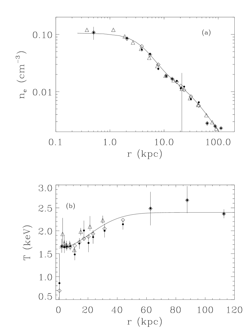
Figure 4: (a) Electron density derived with the deprojection method (filled circles). The open diamonds represent the $n_{e}$ profile after the smoothing operation. The solid line is the best fit profile where a 2-$\beta$ model (see eq. 2) has been used. (b) Deprojected temperature profile versus radius (filled circles). The open diamonds represent the $T$ profile after the smoothing operation. The solid line is the best fit where the expression given in eq. (3) has been used. Error bars in both the panels have been obtained by 1000 Monte Carlo simulations on initial $EI$ and $T_{EW}$. The details on the smoothing operation and on the determination of the error bars are discussed in §4.1. The triangles are the deprojected density and temperature profiles derived by Matsushita et al. (2002).

Following the prescription described in the previous Section, we derive $\varepsilon$, $n_{e}$ and $T$ profiles for M87. All the extracted values are reported in Table 2. In Fig. 4 we plot (filled circles) the deprojected electron density $n_{e}$ and temperature $T$, respectively in panel (a) and (b). For comparison, in Fig. 4 we overplot (open triangles) the deprojected profiles obtained by Matsushita et al. (2002) who used a different choice of regions and a somewhat different technique for spectral deprojection. The Matsushita et al. (2002) results plotted here are those obtained by fitting the MOS data with a 2T model. Our profiles are in reasonable agreement with those derived by Matsushita et al. (2002).

Particular attention must be paid in the computation of the error bars for $T$ and $n_{e}$. In evaluating errors, we want to consider that, even if the deprojection technique assumes that the spherical symmetry condition is fulfilled, the dispersion of the $EI$ and $T_{EW}$ measurements along each ring around the averaged value is often significantly larger than the error of each measure. In particular, this occurs for the XMM-Newton  data, since the XMM-Newton  large effective area allows a very good statistics for M87 and provides $EI$ measurements with very small error bars. The scatter of the data around the averaged value of the ring is a measure of the data displacement from the spherical symmetry. In order to account for this displacement in the final error evaluation, we decided to assign to the $EI$ and $T_{EW}$ of each region, an error ($\sigma_{EI}$ and $\sigma_{T_{EW}}$ respectively) which is the linear sum of two different contributions. The first contribution is simply the error derived from the spectral fit with the 1T/2T model. The second contribution is given by the dispersion of the measurements along the ring around the averaged value. Error bars for the deprojected quantities $n_{e}$ and $T$ reported in Fig. 4 have been obtained running 1000 Monte-Carlo simulations, sampling the $EI$ and $T_{EW}$ of each region around their mean value assuming Gaussian distributions for the errors $\sigma_{EI}$ and $\sigma_{T_{EW}}$.

The profiles plotted in Fig. 4 will be used as starting points to derive some other quantities (such as mass and conductivity). In most cases, gradients of $n_{e}$ and $T$ are involved. Some smoothing procedure will be required to manage these derivatives. Consequently, we apply a smoothing algorithm which replaces each point with the average value obtained using boxes of 3 points, i.e.: $V_{i}=\left(V_{i-1}+V_{i}+V_{i+1}\right)/3$. In smoothing the temperature profile, we excluded from the smoothing procedure the two last (Beppo-SAX) points, in order to preserve the final decreasing behavior of the $T$ profile. The final temperature profile is obtained by applying the smoothing procedure twice: firstly, we smooth the starting deprojected profile and then the obtained values are smoothed again. For the density profile, we applied the smoothing procedure separately to the first 6 points and the others in order to preserve the 2-$\beta$ behavior. Again the two last points have been excluded from the smoothing operation and the smoothing has been applied twice. The open diamonds in Fig. 4 represent the $n_{e}$ and $T$ profile after the smoothing operation. An alternative solution to smoothing is provided by the use of analytical functions fitting the profiles. The solid lines in the figures are the best fits to the data. For the electron density profile we use the fitting function:

$$n_{e}(r)={{n_{1}}\over{\left[1+\left({r\over{r_{1}}}\right)^{2}\right]^{\alpha_{1}}}}+{{n_{2}}\over{\left[1+\left({r\over{r_{2}}}\right)^{2}\right]^{\alpha_{2}}}},$$ (2)

which corresponds to a 2-$\beta$ model. For the temperature profile we find that the function

$$T(r)=T_{0}-T_{1}\exp\left(-{{r^{2}}\over{2\sigma_{T}^{2}}}\right)$$ (3)

provides a good description of the data. For the temperature profile, we find the following best-fit values: $T_{0}=2.399\pm 0.090$ keV, $T_{1}=0.776\pm 0.097$ keV, $\sigma_{T}=3.887^{\prime}\pm 0.731^{\prime}$. For what concerns the electron density, we find $r_{1}=2.68^{\prime}\pm 0.54^{\prime}$, $\alpha_{1}=0.71\pm 0.06$, $n_{1}=0.033\pm 0.01$ cm^-3, $r_{2}=3.73^{\prime}\pm 9.65^{\prime}$, $\alpha_{2}=20.19\pm 104.84$ and $n_{2}=0.069\pm 0.010$ cm^-3. The inferred best fit values have large statistical errors. This is due to the large number of free parameters adopted. So, we decided to fix two parameters, namely, the core radius and the slope of the second component; we fix the slope at large radii $\alpha_{2}$ to the value obtained from the RASS measurements (Böhringer et al., 1994) setting $\alpha_{2}=0.705$ ($\beta=0.47$). For the radius $r_{2}$ we decided to use the value of the $\sigma_{T}$ inferred from the best fit of the temperature profile, which defines the scale radius for the rise of the temperature. Having fixed the values of $r_{2}$ and $\alpha_{2}$, we find: $\alpha_{1}=1.518\pm 0.317$, $n_{1}=0.089\pm 0.011$ cm^-3, $r_{1}=0.834^{\prime}\pm 0.175^{\prime}$ and $n_{2}=0.019\pm 0.002$ cm^-3. Note that the inferred value of $r_{1}$ ($\sim 5$ kpc) roughly corresponds to the AGN jet extension (e.g. Di Matteo et al., 2003; Young et al., 2002).

4.2 Sector deprojection

The deprojection method is based on the assumption of spherical symmetry. As discussed in §2, the hot component in those regions which are described by the 2 temperature (2T) model behaves very similarly to the gas in the regions described by a single temperature (1T) model. However, we should like to verify if any correlation of the hot component with the radio emission exists, invalidating our assumption of spherical symmetry. To this aim, we divided the cluster in sectors and deprojected separately each sector. Again we consider only the hot component for the 2T regions. The sectors have been chosen according to the radio emission regions: the $[30^{\circ}-120^{\circ}]$, $[210^{\circ}-270^{\circ}]$ and $[330^{\circ}-360^{\circ}]$ sectors have been cumulated together to form the non-radio sector. Furthermore, we analyzed separately each of the following sectors: $[0^{\circ}-30^{\circ}]$, $[120^{\circ}-150^{\circ}]$, $[270^{\circ}-300^{\circ}]$, $[300^{\circ}-330^{\circ}]$ which correspond or are close to the radio emission arms.

The Chandra data are not suitable to perform such a study, because the statistics is not very high. In this case, possible azimuthal variations can be hidden by errors. Therefore, in order to verify the assumption of spherical symmetry, we consider only the XMM-Newton  data (circles in Fig. 2). Nevertheless, also with XMM-Newton  data, it is quite difficult to use small sectors to perform sector-by-sector comparisons since their statistics is not very high. A significant comparison can be made between the whole cluster and the non-radio selected sector. In Fig. 5 (in panel (a) and (b) respectively) we compare the $n_{e}$ and $T$ profiles for the whole cluster (filled dots) with the non-radio sector (open diamonds). In general, no significant differences are evident. The profiles of the electron density are almost identical whereas there is a slight tendency of the temperature calculated on the whole cluster to be smaller than the temperature of the non-radio sector. The difference is due to the fact that in the non-radio sector only 1T regions contribute, while in the whole cluster profile also the contribution of the hot component temperature of the regions described by a 2T model is accounted. This temperature is slightly smaller than the overall temperature and produces a mild decrease of the whole cluster temperature profile with respect to the non-radio sector temperature profiles. However, differences are well within 1$\sigma$; thus, excluding the radio emission sectors (or the regions described by the 2T model) does not affect significantly the results and no evident azimuthal asymmetry can be highlighted. We can conclude that the spherical symmetry assumption, which is an important condition for our analysis, is tenable. It is also worth noting that, in order to derive most of the other physical quantities (mass, conduction, entropy, etc.) a smoothing operation on $T$ and $n_{e}$ is necessary, so that the small differences reported above would not anyhow affect our results.

4.3 The gravitational mass for M87

Once the basic quantities $n_{e}$ and $T$ are obtained through the deprojection, under suitable assumptions, other related quantities describing the ICM can be derived. One of the most important is the gravitational mass. Supposing that the gas is in hydrostatic equilibrium within the potential well of the dark matter, the gravitational mass $M$ within a radius $r$ can be derived via the hydrostatic equilibrium equation:

$$M(<r)=-{{kTr}\over{G\mu m_{p}}}\left[{{d\ln{T}}\over{d\ln{r}}}+{{d\ln{n_{e}}}\over{d\ln{r}}}\right]$$ (4)

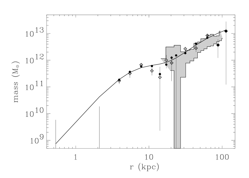
Figure 6: Gravitational mass derived through the hydrostatic equilibrium equation. The filled circles refer to the profile inferred by smoothing the temperature and the density profiles. The open diamonds plot the gravitational mass derived without any smoothing operation on $n_{e}$ and $T$, errors have been derived using the standard Monte Carlo technique. Three of these points have values near to zero and only the upper limit of their error bar has been plotted here. The solid curve is the analytical mass obtained using the best fit profiles for $n_{e}$ and $T$ (eqs. 2 and 3). For comparison, the grey-shaded regions report the gravitational mass derived by Nulsen and Böhringer (1995) using ROSAT–PSPC data.

where $\mu=0.6$ is the mean molecular weight, $G$ the gravitational constant and $m_{p}$ the proton mass. Even if eq. (4) provides a direct method to derive the gravitational mass, it is a differential equation and the temperature and the electron density are involved through their gradients. Irregular features in the profile induce jumps on the evaluated mass. A classic solution consists in smoothing the data and replacing the $n_{e}$ and the $T$ profiles with their smoothed counterparts plotted in Fig. 4 (open diamonds). As far as the temperature is concerned, a smoothing procedure is viable since errors are rather large and the general shape of the profile is quite smooth. Correspondingly, the smoothed profile is compatible (always within 1$\sigma$) with the original one. On the contrary, for the electron density where errors are small, the smoothing procedure could hide some features which are physical. In order to assess whether the smoothing affects results, we compare the gravitational mass obtained using the temperature and the density smoothed profiles with the gravitational mass derived using the unsmoothed profiles where errors have been evaluated using the standard Monte Carlo technique. As we show in Fig. 6, the smoothed profile (filled circles) agrees with the non-smoothed one (open diamonds) within $1-2\sigma$ and no significant difference can be highlighted. It is worth noting that the mass derived without smoothing provides three mass values (at $r\sim 0.5,\sim 2$ and $\sim 25$ kpc) which are negative and compatible with zero: $M=-0.5^{+1.1}_{-1.4}\times 10^{10}{\rm M_{\odot}}$, $M=-2.7^{+9.6}_{-4.7}\times 10^{10}{\rm M_{\odot}}$ and $M=-0.22^{+1.45}_{-1.67}\times 10^{12}{\rm M_{\odot}}$. For these points, in Fig. 6, we show only the upper limit of the error bar.

Alternatively to the smoothing procedure, the analytical expressions for $n_{e}$ and $T$ (eqs. 2 and 3) can be used. The curve in Fig. 6 is the analytical mass obtained using these two best fit profiles. This mass profile has a plateaux at a radius of about $10-15$ kpc ($\sim 2$ arcmin). This flattening behavior is the consequence of the flattening of the 2-$\beta$ profile, at the same radius, which could correspond to the edge of the central cD. The analytical gravitational mass is very similar to the mass obtained both with the smoothing procedure and with the unsmoothed data. The differences with respect to the latter curve are limited to a few points ($\sim 15,\sim 25$ and $\sim 90$ kpc). For these points, some “holes” appear in the shape of the non-analytical profiles. It is worth noting that the “hole” in a (integrated) mass profile is not physical. It may indicate that in this region the hydrostatic equilibrium hypothesis breaks down (e.g. Pizzolato et al., 2003) and that an outflow providing additional pressure to support gravity occurs there (see next Section for equations and further details). In any case, the error bars of all these points are large enough to make “holes” compatible with the analytical profile and no strong evidence is present to claim that an outflow is present.

For comparison, the grey-shaded regions in Fig. 6 report the gravitational mass derived by Nulsen and Böhringer (1995) using ROSAT–PSPC data. Our profile, in the common radial regions is in agreement. It is interesting to note that the point at $r\sim 20$ kpc has a very large error bar in both the estimations.

5 Cooling, conduction and heating

As previously outlined, finding a heating mechanism able to balance the cooling is not an easy task. This Section will be devoted to the inspection of some heating sources using the M87 data set.

The heating contribution required to balance the radiative cooling can be estimated starting from the thermodynamic equations describing a spherically symmetric cluster:

$$\frac{1}{r^{2}}{d\over{dr}}(\rho vr^{2})=0$$

$$\rho v{dv\over{dr}}+{d\over{dr}}\left({{\rho kT}\over{\mu m_{p}}}\right)+{{GM}\over r^{2}}\rho=0$$ (5)

$$\frac{1}{r^{2}}{d\over{dr}}\left[r^{2}\rho v\left(\frac{1}{2}v^{2}+\frac{5}{2}{{kT}\over{\mu m_{p}}}+\phi\right)\right]=-\varepsilon+\varepsilon_{cond}+\cal{H}$$

where $\phi$ is the gravitational potential, $M$ the gravitational mass within $r$, $T$ the gas temperature, $\varepsilon$ the emissivity and $\rho$ the gas mass density which is related to the electron density according to $n_{p}=0.82n_{e}=\rho/(2.21\mu m_{p})$ ($\mu=0.6$ is the mean molecular weight). The equations take into account the possible presence of an inflow or outflow and the flow velocity $v$ is taken positive outwards.

The three equations (5) are respectively the mass, momentum and energy conservation equations. They have been derived (see Sarazin, 1988) assuming a steady state; the second equation reduces to hydrostatic equilibrium, eq. (4), for $v=0$. We include in the right-hand-side of the last equation, the radiative cooling $\varepsilon$, and a heat contribution which includes two parts: the thermal conduction $\varepsilon_{cond}$ which will be widely discussed in the next paragraph, and a generic extra-heating term $\cal{H}$, which will be studied in detail in Section 5.2.

5.1 Radiative cooling and conduction

One obvious heating source is the thermal conduction which operates when temperature gradients occur, and which can have a relatively large efficiency (a fraction of the Spitzer conduction) even in presence of magnetic fields (Gruzinov, 2002; Narayan and Medvedev, 2001).

Neglecting any extra-heating source ($\cal{H}$ $=0$ in eq. 5), and under the assumption of a spherical, steady state, isobaric cooling flow, the last equation of (5) can be rewritten in the form:

$$-{{\dot{M}}\over{4\pi r^{2}}}{d\over{dr}}\left({{5kT}\over{2\mu m_{p}}}\right)=-\varepsilon+\varepsilon_{cond}\,.$$ (6)

where $\varepsilon$ is the emissivity, $\mu=0.6$ is the mean molecular weight and $\dot{M}$ is the usual mass deposition rate of the cooling flow.

The heating due to thermal conduction $\varepsilon_{cond}$ is given by:

$$\varepsilon_{cond}=\frac{1}{r^{2}}{d\over{dr}}\left(r^{2}\kappa{{dT}\over{dr}}\right),$$ (7)

where $\kappa$ is the conductivity. For a highly ionized plasma, $\kappa$ is given by the Spitzer (1962) formula:

$$\kappa=\kappa_{S}={{1.84\times 10^{-5}\left(T/{\rm\kern 2.0pt{}^{\circ}{\kern-0.5ptK}}\right)^{5/2}}\over{\ln{\Lambda}}}{\rm\,erg\,cm^{-1}\,s^{-1}\,\kern 2.0pt{}^{\circ}{\kern-0.5ptK}^{-1}}\,,$$ (8)

where $\ln{\Lambda}\sim 40$ is the usual Coulomb logarithm.

Starting from these equations we can derive the conductivity $\kappa$ required in M87 to stop the cooling flow ($\dot{M}=0$). The inferred values for $\kappa$ are plotted in Fig. 7 (filled circles). We plot $\kappa$ as a function of the temperature in order to compare our results with Voigt et al. (2002) and Voigt and Fabian (2004) who have performed a similar calculation on a set of clusters. We recall that the temperature grows with the radius. Hence, the behavior of $\kappa$ as a function of the temperature is similar to the behavior of the profile of $\kappa$ as a function of the radius. From Fig. 7 we can see that the required conductivity has large values for small temperatures (i.e. in the central part of the cluster) and becomes smaller when the temperature increases, i.e. moving towards the outskirts of the cluster. Note that the temperature profile in the innermost regions of the cluster is consistent with being constant. Correspondingly, no conduction should be present and the required conductivity is consistent with being as high as infinity. Hence, for these points, error bars will extent to infinity. In order to show in Fig. 7 that the error bar for these points should extent to infinity, we plot their error bars with an arrow. The solid line in Fig. 7 represents $\kappa_{S}$ given in eq. (8) and dashed line corresponds to 0.3$\kappa_{S}$ which could be the effective conductivity in presence of turbulent magnetic fields (Gruzinov, 2002). Fig. 7 shows that in M87, the thermal conduction is able to balance radiative cooling only in the outer part of the cluster. For $r\lower 2.15277pt\hbox{$\;\buildrel>\over{\sim}\;$}10-20$ kpc the conductivity required for conduction to balance the cooling is between 0.3$\kappa_{S}$ and $\kappa_{S}$. In the inner $\sim 10-20$ kpc in M87 the heating supplied by thermal conduction is not enough and an extra-heating, whatever its source might be, is needed. The failure of the thermal conduction in the core of the cluster is due to the fact that in these regions the temperature profile flattens (see Fig. 4b) and the conduction decreases substantially. At the same time, the innermost regions are those where the X-ray emissivity is highest and which mostly require a heating source to compensate the radiated energy.

In a recent paper, Voigt et al. (2002) determined the conductivity required for the conduction to balance the radiation losses for A2199 whose temperature is similar to M87 temperature ranging from $\sim 2$ to $\sim 5$ keV. For comparison, we plot in Fig. 7 the Voigt et al. (2002) data for A2199 derived by modeling the temperature profile with two different prescriptions: a power law (triangles) and a more complex functional form (squares) which flattens at small and large radii (see eq. (6) in Voigt et al., 2002). Because of the larger distance of A2199 ($z=0.0309$) only a couple of points are within the central 10 kpc. Nevertheless, in agreement with our results, they find that for these two central bins some extra-heating is needed. The quality of the M87 data set allows to highlight the problem of conduction in the core and to analyze it in greater detail than for A2199. Clearly, M87 is a good object to test heating models. In Fig. 7 we also plot (open circles) the $\kappa$ values obtained for M87 by Voigt and Fabian (2004). Their values are in reasonable agreement with ours, although their analysis procedure is quite different from ours. In Voigt and Fabian (2004) only Chandra data are included limiting the extension of the deprojected region to the inner 10 kpc and only the 1T xspec - mekal model is used in fitting spectra extracted from annuli.

5.2 Heating for M87 and the “effervescent” heating model

In this Section we consider eqs. (5) in their generic form in order to determine the extra-heating $\cal{H}$ required to balance the radiative cooling in presence of thermal conduction for M87.

Eqs. (5) can be recasted in the form:

$$v\rho r^{2}=const={{\dot{M}}\over{4\pi}}$$

$$M=-{{r^{2}v}\over{G}}{{dv}\over{dr}}-{{kTr}\over{G\mu m_{p}}}\left[{{d\ln{T}}\over{d\ln{r}}}+{{d\ln{n_{e}}}\over{d\ln{r}}}\right]$$ (9)

$${\cal{H}}=\varepsilon-\varepsilon_{cond}+\varepsilon^{\star}$$

where we set:

$$\varepsilon^{\star}={{\rho vkT}\over{\mu m_{p}r}}\left[\frac{3}{2}{{d\ln{T}}\over{d\ln{r}}}-{{d\ln{\rho}}\over{d\ln{r}}}\right]\,.$$ (10)

This term includes the variation of the energy (per unit volume) due to the outflow/inflow and the work (per unit volume) done by the system during the outflow/inflow. The mass flow rate $\dot{M}$ is positive for an outflow and negative for an inflow. The last equation of (9) provides the heating $\cal{H}$ necessary to balance the radiative cooling $\varepsilon$, in presence of thermal conduction and steady outflow. The deprojected data $T$, $n_{e}$ (or $\rho$), of M87 can be used to solve numerically eqs. (9) for M87, deriving $M$, $v$ and $\cal{H}$, once we have fixed the fraction $f$ of the Spitzer conductivity (eq. 8) and some assumption has been made on $\dot{M}$. We fix an $f=0.3$ efficiency (see Gruzinov, 2002) and we set the outflow mass rate $\dot{M}=1.6{\rm M_{\odot}/yr}$. This $\dot{M}$ value is similar to the asymptotic value that RB02 obtained from their simulations for the stable final state of the cluster. We will discuss further on different values for $\dot{M}$ and $f$.

As far as the velocity is concerned, for the assumed values of $f$ and $\dot{M}$, $v$ is smaller than a few tens of km/s, for radii larger than $\sim 1-2$ kpc. Correspondingly, the term including the velocity in the momentum conservation equation (the second equation of 9) is significantly smaller than the total mass being of the order of $10^{5}-10^{7}\,{\rm M}_{\odot}$ versus the $10^{10}-10^{12}\,{\rm M}_{\odot}$ of the total mass, so its contribution is negligible. Hence, we can state that the cluster is almost in hydrostatic equilibrium and the mass estimates reported in Fig. 6, where the term related to the outflow is neglected, are not affected. In order to have a significant contribution from the velocity term and to alter substantially the hydrostatic equilibrium, $\dot{M}$ values as large as several tens–few hundreds of ${\rm M}_{\odot}/{\rm yr}$ are required.

For the considered values of $\dot{M}$, the quantity $\varepsilon^{\star}$ in eq. (10) is negligible with respect to the emissivity $\varepsilon$. Thus, the extra-heating $\cal{H}$ and the conduction term $\varepsilon_{cond}$ are completely used to balance the radiative cooling.

For what concerns $\cal{H}$, the heating required in M87 is plotted in Fig. 8 (filled circles). As expected, most of the heating is required in the central part of the cluster (say in the inner $\sim 15-20$ kpc), where conduction is not efficient. The heating due to thermal conduction is plotted in Fig. 8 (dot-dashed line); in the central $10$ kpc, where the temperature profile becomes flatter, the thermal conduction drops to zero, apart from the innermost bin ($\sim 1$ kpc) where $T$ falls to very small values (see Fig. 4b), with a large error bar. The conduction in this bin is $\varepsilon_{cond}=1.46^{+1.89}_{-1.53}\times 10^{-24}{\rm erg\,cm^{-3}s^{-1}}$, and is in agreement with zero within 1$\sigma$.

The heating model developed in Ruszkowski and Begelman (2002, RB02 hereafter) and Begelman (2001) includes a mechanism for heat injection from the central AGN. The mechanism has been called “effervescent heating”. The radio source is supposed to deposit some buoyant gas bubbles in the ICM, which do not mix and rise through the ICM microscopically. The bubbles should expand doing work on the surrounding plasma and converting their internal energy in heat. The buoyant outflow contribution in the energy conservation equation is accounted for in the $\varepsilon^{\star}$ term, while $\cal{H}$ describes the heat injection due to the adiabatic expansion of the bubbles.

According to the RB02 model, the heating $\cal{H}$ is a function of the pressure (and its gradient) and can be expressed according to:

$${\cal{H}}=-h(r)\left({p\over p_{0}}\right)^{(\gamma_{b}-1)/\gamma_{b}}\frac{1}{r}{{d\ln{p}}\over{d\ln{r}}},$$ (11)

where,

$$h(r)={L\over{4\pi r^{2}}}\left(1-e^{-r/r_{0}}\right)q^{-1}$$ (12)

and

$$q=\int_{0}^{+\infty}{\left({p\over{p_{0}}}\right)^{(\gamma_{b}-1)/\gamma_{b}}\frac{1}{r}{{d\ln{p}}\over{d\ln{r}}}\left(1-e^{-r/r_{0}}\right)dr}\,;$$ (13)

$p$ is the pressure, $p_{0}$ is the central pressure, $L$ the time-averaged luminosity of the central source, $\gamma_{b}$ is the adiabatic index of the buoyant gas and $r_{0}$ the inner heating cutoff radius. The term $1-exp(-r/r_{0})$ introduces an inner cutoff which fixes the scale radius where the bubbles start rising buoyantly in the ambient plasma. $\cal{H}$ is normalized in such a way that, when integrated over the whole cluster, the total injected power corresponds to the time-averaged power output of the AGN. $\cal{H}$ has been derived in eq. (11) assuming a steady state for the bubble flux. In order to assess if this assumption is reasonable we must compare the different timescales involved in the effervescent heating mechanism. We can suppose that the AGN is intermittent (RB02; Reynolds and Begelman, 1997) and heats the ICM through a succession of outbursts. During each outburst, the AGN injects a population of bubbles which subsequently rise buoyantly. During the “off” periods, the bubbles continue their rise heating the cluster atmosphere. If the outbursts follow each other on a timescale which is short with respect to the rising timescale of the bubbles, then the flux of the bubbles reaches a quasi steady state. In fact, the ratio $t_{rise}/t_{i}$ between the rise timescale $t_{rise}$ and the intermittence timescale $t_{i}$ gives the number of populations injected within the ICM within a time $t_{rise}$. The larger this ratio is, the larger the number of bubble populations rising into the cluster atmosphere and the mechanism approaches the steady state. The radio galaxies are likely to be intermittent on a timescale as short as $t_{i}\sim 10^{4}-10^{5}$ yr (RB02; Reynolds and Begelman, 1997). In the next section we will see that the risetime is $t_{rise}\sim 10^{8}$ yr or even larger. The value of the ratio $t_{rise}/t_{i}$ is $10^{3}-10^{4}$ or more; therefore the assumption of steady state is tenable and the released heating may be treated in a time-averaged sense.

RB02 also include a convection term in eq. (9) which we have neglected. The reason for this choice is twofold. First of all, the convection must be limited to the innermost regions of the cluster, in order to allow the presence of metallicity gradients in cluster cores (De Grandi and Molendi, 2001). Most importantly, a negative gradient for the entropy is a necessary condition for the onset of the convection. In fact, the condition of instability:

$${d\over dr}\left({p\over{\rho^{\gamma}}}\right)<0$$ (14)

(where $\gamma$ is the ratio of the specific heats $c_{p}/c_{v}$ and has the value $5/3$ for a highly ionized gas) must be fulfilled for the convection to operate and it is equivalent to requiring that $\nabla(T/n^{2/3})<0$. This condition is not satisfied in M87 where we verified that the entropy is an increasing function of the radius, as we show in Fig. 9.

We compare the values inferred for the extra-heating $\cal{H}$ term in M87 reported in Fig. 8 (filled circles), with the predictions from the RB02 model derived according to eq. (11), in order to assess whether, for a reasonable choice of the parameters, the heat flux required to balance the cooling is compatible with the heat injected by the central AGN.

In order to determine the pressure and the pressure gradient in eq. (11), we use the analytical expressions (2) and (3) for $n_{e}$ and $T$ with the best-fit parameters obtained by fitting the deprojected electron density and temperature profiles. We use eqs. (11) - (13) as fitting functions for the extra-heating, where $\gamma_{b}$, $r_{0}$ and the total normalization $A$:

$$A={L\over{4\pi}}q^{-1}$$ (15)

are the free parameters. The solid line in Fig. 8 is the derived best fit. The model proposed by RB02 seems to provide a fair description of the heating needed to balance the cooling flow in the inner $\sim 15-20$ kpc of the cluster, where conduction is not sufficient. The line seems to follow adequately the behavior of the data points. Nevertheless, the derived fit values have large errors. By fixing $\gamma_{b}=4/3$ (which is the adiabatic index for relativistic bubbles), we find $r_{0}=4.39\pm 1.83$ kpc and $A=(8.35\pm 1.65)\times 10^{-24}\,{\rm erg\,s^{-1}}$ (the dashed curve in Fig. 8). By using eq. (15), we can also derive the central AGN luminosity $L=5.95\times 10^{42}\,$ ${\rm erg\,s^{-1}}$ required to stop the cooling.

The three external points in Fig. 8 seem to require an additional extra heating, showing an excess with respect to the general behavior of the data at large radii and with respect to the best fit function shape. This excess is related to the flattening of the temperature profile in the external regions which dampens conduction. However, it must be noted that the values of the heating $\cal{H}$ required in these three bins are respectively: $2.32^{+0.89}_{-0.80}\times 10^{-28}{\rm erg\,cm^{-3}s^{-1}}$, $5.32^{+3.51}_{-4.07}\times 10^{-28}{\rm erg\,cm^{-3}s^{-1}}$ and $6.56^{+4.14}_{-5.31}\times 10^{-28}{\rm erg\,cm^{-3}s^{-1}}$ and are all in agreement with zero within $2-3\sigma$. Hence, the evidence for the excess is not particularly strong.

Our estimated radius $r_{0}\sim 4-5$ kpc, is comparable to the extension of the AGN jet as seen in the Chandra image of M87 (e.g. Di Matteo et al., 2003; Young et al., 2002). The fact that $r_{0}$ is of the same order of magnitude of the jet is consistent with a scenario where the effervescent bubbles are generated through the interaction of the radio jet with the cluster atmosphere. Understanding the precise nature of such interaction will require considerable efforts both on the observational and theoretical side. Our aim here is simply to note that our fit does not rule out the possibility that the bubbles are generated through the interaction of the radio jet with the cluster atmosphere, as would have been the case if, for example, the fitting of the effervescent model to M87 had returned an $r_{0}$ value 10 times larger than the one actually measured. The inferred luminosity value is similar to the luminosity evaluated for the M87 AGN (Owen, Eilek and Kassim, 2000, OEK hereafter), $\sim 3-4\times 10^{42}{\rm erg\,s^{-1}}$ (see also Di Matteo et al., 2003). Slightly different values for the luminosity could be inferred with different choices of $f$ and $\dot{M}$ which of course provide different best fit parameters values and different related luminosities. When a larger $f$ is considered, the higher contribution of the thermal conduction reduces the amount of heating needed to balance the radiative cooling. Setting the conductivity to the Spitzer value ($f=1$) we find best fit values which are similar to those inferred for $f=0.3$ and provide a slightly lower luminosity ($\sim 2-3\times 10^{42}{\rm erg\,s^{-1}}$). On the contrary, when smaller values for $f$ are considered, some additional heating is necessary. For $f=0.1$ we derive an AGN luminosity $\sim 1-2\times 10^{43}{\rm\,erg\,s^{-1}}$, which is somewhat larger than the OEK estimations. However, for such small efficiencies, the shape of the RB02 model no longer provides a good description of the data, especially in the central regions. Thus, if the contribution of the thermal conduction is too small, the “effervescent heating” model is not suitable to describe the heating necessary to balance the cooling flow.

Some variations are found also for different initial values of $\dot{M}$. We tried 16 and 0.16 M_⊙/yr corresponding to 10 and 0.1 times the original $\dot{M}$ value we considered. As expected, for large values of $\dot{M}$ the corresponding AGN luminosity is significantly enhanced ($\lower 2.15277pt\hbox{$\;\buildrel>\over{\sim}\;$}few10^{43}\,{\rm erg\,s^{-1}}$) since the central AGN must provide a larger quantity of energy to the outflowing bubbles. The variations when smaller $\dot{M}$ are considered, are modest, slightly reducing the luminosity to $\sim 3-4\times 10^{42}\,{\rm erg\,s^{-1}}$.

Note that it is not necessary for the AGN luminosity, obtained by requiring that the “effervescent heating” model balances the cooling flow to be exactly equal to the AGN luminosity derived from radio observations. In fact, the required luminosity from the model should be regarded as a time-averaged power of the AGN, as the AGN dynamical times are smaller than the radiative cooling flow scale times. One should also keep in mind that only a fraction of the total power of the AGN is used to quench the cooling flow and that the luminosity required from the model can be significantly smaller than the real AGN luminosity. From our analysis, we can infer that the values of $L$ derived with different choices of $f$ and $\dot{M}$ are of the same order of estimates by OEK and Di Matteo et al. (2003).

While the luminosity is slightly affected for different choices of $\dot{M}$ and $f$, $r_{0}$ variations are quite modest and the inferred values of the scale radius are always of the order of $r_{0}\sim 4-5$ kpc, which approximatively corresponds to the AGN jet extension.

5.3 Discussion

Starting from the results inferred in the previous section, we can try to draw a more general picture, using also informations coming from radio observations of M87.

We can suppose that the buoyant bubbles are radio bubbles filled with magnetic field and relativistic particles (Gull and Northover, 1973; Churazov et al., 2000, 2001; Brüggen and Kaiser, 2001; Churazov et al., 2002) responsible for the synchrotron emission in M87. As already outlined by OEK, the radio structures are highly filamented. This suggests that the dimensions of the bubbles are small. Enßlin and Heinz (2002) discussed the dynamics of the rise of buoyant light bubbles within the cluster atmosphere (see also Churazov et al., 2001; Kaiser, 2003). The buoyant bubble rapidly reaches a terminal velocity $v_{b}$. In the limit of small bubbles, $v_{b}$ can be estimated by balancing the buoyancy force with the ram pressure (drag force) of the cluster gas.

The buoyancy force is

$$F_{b}=Vg(\rho-\rho_{b})\,=Vg\rho\Delta\,,$$ (16)

where $V=4/3\pi r_{b}^{3}$ is the volume of the bubble, $r_{b}$ is the bubble radius, $g=GM(<r)/r^{2}$ is the local gravity acceleration at the radius $r$ ($M$ is the gravitational mass within the radius $r$); $\rho$ and $\rho_{b}$ are respectively the density of the ICM and of the bubble. $\Delta=(\rho-\rho_{b})/\rho$ is the density contrast.

The drag force for subsonic motion can be approximated by

$$F_{drag}=C\pi r_{b}^{2}\rho v_{b}^{2}$$ (17)

with the drag coefficient $C\simeq 0.5$.

By equating eqs. (16) and (17) the velocity of the bubble can be determined. Enßlin and Heinz (2002) derived $v_{b}$ under the assumption that the density of the ICM is well described by an isothermal $\beta$-model and the density contrast $\Delta\sim 1$. In this case $v_{b}$ is a fraction ($\propto\sqrt{r_{b}/r_{c}}$; $r_{c}$ is the core radius of the cluster) of the sound velocity. Correspondingly, for small bubbles, $v_{b}$ is subsonic which is consistent with the fact that no shocks are detected in M87.

We derived the rise velocity of the bubbles in M87 at a radius $r\sim 10$ kpc, using the results from the deprojection for $M(<r)$ and $\rho$. The density contrast $\Delta$ can be inferred considering that the bubbles filled with relativistic plasma are in pressure equilibrium with the ICM. Indeed, the pressure equilibrium between radio bubbles and thermal plasma implies that $n_{e}kT\sim\beta n_{er}\langle E_{e}\rangle$ (where $\beta$ is a factor of the order of the unity which accounts for the contribution to the pressure of the magnetic field which is almost in equipartition with the particle energy). $\langle E_{e}\rangle$ is the mean energy of the relativistic particles and $n_{er}$ is the numerical density of the relativistic particles. The relativistic particles mean energy is much larger than that of the thermal electrons in the ICM, leading to a density contrast $\Delta\sim 1$. The values of $v_{b}$ for the bubble radius $r_{b}$ varying in $[0.01-1.]$ kpc range are plotted in Fig. 10 and the motion is indeed subsonic.

It is worth considering that, in a recent analysis of these data (Molendi, 2002, M02 hereafter), we have found that, cospatially with the radio lobes, there exists a thermal component with $T\sim{1\over 2}T_{ICM}$. This component is likely structured in blobs with typical scales smaller than $\sim 100$ pc. The filling factor of these blobs has been estimated to be of the order of the percent.

Some informations about the filling factor of the radio bubbles can be obtained using recent results from radio observation of M87. Using the standard minimum pressure analysis (e.g. Pacholczyk, 1970; Burns, Owen and Rudnick, 1979; O’Dea and Owen, 1987), OEK evaluate the magnetic field in the lobes and in the filaments visible in the radio map and evaluate the minimum pressure of the magnetic field and relativistic particles. They assume that the proton-to-electron energy is $k=1$ and that $\zeta\phi=1$ where $\phi$ is the filling factor of the relativistic particles and of the magnetic field and $\zeta$ is the ratio of the true magnetic pressure (comprehensive of the tension) to the magnetic pressure $B^{2}/8\pi$. For a tangled magnetic field $\zeta=1/3$. The estimations for the minimum pressure derived by OEK can be compared with the thermal pressure that we can infer from our deprojected $T$ and $n_{e}$ profiles. In agreement with OEK, we find that the pressure of the relativistic plasma is smaller than the thermal pressure by about an order of magnitude. By keeping the condition $k=1$ and assuming $\zeta=1$, we can derive the filling factor which reconciles the minimum pressure $P_{min}$ with the thermal pressure of the plasma, considering that the minimum pressure scales with $\phi$ according to:

$${{P_{min}(\phi)}\over{P_{min}(\phi=1)}}=\left(\phi\right)^{-4/7}\,.$$ (18)

The discrepancy of a factor $\sim 10$ between the two pressures can be eliminated by assuming a filling factor $\sim 1\%$. By using the estimations of $P_{min}$ from OEK in different plasma of the radio lobes and filaments, we infer filling factors of few $\%$. Assuming $\zeta=1/3$ (tangled magnetic field) reduces $\phi$ by a factor $\sim 2$. The filling factors of the radio bubbles and of the cold thermal blobs are of the same order.

The survival of the cold thermal blobs in the hotter ICM requires that thermal conduction be substantially suppressed; this may happen if these blobs are tied to the radio bubbles and magnetic fields shield them from collisions with ICM particles. Since the filling factors of blobs and bubbles are similar and the density of the blobs is about twice that of the ICM (M02), the mean density of each bubble+blob is about that of the surrounding ICM. Thus, assuming that the blobs are tied to the bubbles and that they occupy similar volumes, their density contrast with the surrounding ICM will be small. In Fig. 10 the dotted line plots the bubble rise velocity $v_{b}$ for a $\Delta=0.1$. Starting from the rise velocity, it is straightforward to derive the rise timescale of the bubbles. For a density $\Delta\sim 1$ and a bubble radius of $\sim 100$ pc, the risetime is $t_{rise}\sim 10^{8}$ yr at $r\sim 10$ kpc and it becomes even larger for smaller bubbles and smaller density contrasts, holding $t_{rise}\propto{(r_{b}\Delta)}^{-1/2}$. As outlined previously, this value is significantly larger than the duty cycle timescale $t_{i}$ of intermittency of the AGN, so that the ratio $t_{rise}/t_{i}\lower 2.15277pt\hbox{$\;\buildrel>\over{\sim}\;$}10^{3}-10^{4}$ and the mechanism approaches the steady state.

It is worth noting that the above picture refers to radio bubbles and cool X-ray blobs located in the lobes. However, the heating process related to the rise of the bubbles must be isotropic throughout the cluster in order to balance the cooling flow. Under the assumption that the radio galaxy is intermittent on a short timescale, the mechanism is expected to heat isotropically the ICM since it is likely that no direction is preferred for the AGN ejection; we also recall that when the AGN is turned off the bubbles continue their rise within the ICM heating it up; within this picture, by averaging on a cooling time, the radio bubble populations are likely to be isotropically distributed in the cluster.

Nevertheless, the cool X–ray blobs are detected only in the lobes regions. So the picture emerging here is that of an AGN which injects radio bubbles, in all the directions, through a succession of outbursts. In the lobes, the outburst is occurring at the present time and, here, also the cool X-ray blobs are present. They are tied to the radio bubbles and the magnetic fields shield them from collisions with ICM particles. The thermal conduction is inhibited allowing the cool blobs to survive in a hotter ambient medium. In the halo, where the radio bubbles have been injected during a past activity of the AGN, only “old” populations of bubbles which are buoyantly rising are present. It is likely that the cool blobs which were tied to the radio bubbles when the AGN was active there, have thermalized, the magnetic fields slow down but do not stop entirely thermalization so that only a single phase gas is detected in the halo regions.

6 Summary

The crisis of the standard cooling flow model brought about by Chandra and XMM-Newton  observations of galaxy clusters, has led to the development of several heating models with the aim of identifying a mechanism able to quench the cooling flow.

We have used observations of Virgo/M87 to inspect the dynamics of the gas in the center of the cluster, and to study the heating processes able to balance radiative losses. We combined the observations of three satellites, namely XMM-Newton, Chandra and Beppo-SAX. By means of the spectral deprojection technique, we inferred the profiles for the temperature $T$ and the electron density $n_{e}$ for M87. The temperature profile drops by a factor of $\sim 2$ in the inner ($\lower 2.15277pt\hbox{$\;\buildrel<\over{\sim}\;$}15$ kpc). The electron density $n_{e}$ is well described by a 2-$\beta$ profile. Starting from these profiles, we derived some related physical quantities such as the gravitational mass and the entropy profile. The gravitational mass profile shows a plateaux at $\sim 10-15$ kpc, which could correspond to the edge of the central cD.

In agreement with Voigt et al. (2002) and Voigt and Fabian (2004) results on a set of cluster, we found that the thermal conduction in M87 can balance the cooling flow only in the outer part of the core (say, $r\lower 2.15277pt\hbox{$\;\buildrel>\over{\sim}\;$}15$ kpc), while in the inner $10-15$ kpc, where the temperature profile becomes flatter and the conduction is no longer efficient, some extra-heating is required. We have determined the extra-heating needed to balance the cooling flow in M87, assuming a thermal conduction efficiency $f=0.3$ with respect to the Spitzer value, and an outflow mass rate $\dot{M}=1.6{\rm M_{\odot}/yr}$. The high quality of our combined dataset allows us to inspect properly the innermost regions, deriving an accurate profile for the extra-heating term $\cal H$ in the regions where thermal conduction is not sufficient to quench the cooling flow.

Several models and simulations concerning heating mechanisms through buoyant gas in the cluster ICM have been recently proposed in the literature (e.g. Ruszkowski and Begelman, 2002; Begelman, 2001; Churazov et al., 2002; Böhringer et al., 2002; Brüggen and Kaiser, 2002a, b; Brüggen et al., 2002). We have assumed that the heating is provided by the central AGN by means of deposition of buoyant bubbles in the ICM according to the model proposed by Ruszkowski and Begelman (2002). The bubbles rise through the ICM and expand doing work on the surrounding plasma and heating it up. We fitted the extra-heating required in M87, with the heating functions proposed by RB02 (see eqs. 11 - 13). The RB02 model seems suitable to describe the behavior of the data. By fixing the adiabatic index $\gamma_{b}=4/3$ (relativistic bubbles), we find a scale radius $r_{0}=4.39\pm 1.83$ kpc and $A=(8.35\pm 1.65)\times 10^{-24}\,{\rm erg\,s^{-1}}$, which corresponds to a central AGN luminosity $L=5.95\times 10^{42}\,{\rm erg\,s^{-1}}$. The scale radius is of the order of the extension of the AGN jet and the inferred AGN luminosity is similar to the one estimated by Owen, Eilek and Kassim (2000) and Di Matteo et al. (2003) $L\sim 3-4\times 10^{42}{\rm erg/s^{-1}}$. Smaller conductivity efficiencies ($f=0.1$) or larger outflow mass rates ($\dot{M}=16{\rm M_{\odot}/yr}$) provide AGN luminosities ($L\sim few10^{43}{\rm\,erg\,s^{-1}}$) which are somewhat higher than the estimations of Owen, Eilek and Kassim (2000) and Di Matteo et al. (2003). However, if the efficiency of the thermal conduction is reduced ($f=0.1$) the model functions of RB02 seem no longer suitable to describe the heating needed to balance the cooling flow. For higher conduction efficiencies ($f=1$) or smaller outflow rates values ($\dot{M}=0.16{\rm M_{\odot}/yr}$) the inferred luminosity is slightly reduced ($L\sim 3-4\times 10^{42}{\rm\,erg/s^{-1}}$). The different values derived for $L$ are of the same order of the luminosity measures for the AGN luminosity in M87 obtained by Owen, Eilek and Kassim (2000) and Di Matteo et al. (2003). In all the cases considered, the inferred scale radius $r_{0}$, which fixes the radius at which bubbles are deposited and start rising, is $r_{0}\sim 4-5$ kpc which approximatively corresponds to the AGN jet extension.

Finally, we discussed a scenario where the bubbles are filled with relativistic particles and magnetic field, responsible for the radio emission in M87. In this scenario the density contrast $\Delta$ is expected to be as large as 1. The buoyant velocity $v_{b}$ of the bubbles can be derived by balancing the buoyant force with the drag force. For small bubbles, the rise velocity is subsonic. Under the hypothesis of equipartition between relativistic particles and magnetic field in the bubbles and of equilibrium pressure with the thermal ICM, we evaluated the filling factor $\phi$ of the radio bubbles. We find $\phi\sim 0.01$ which is of the same order of the filling factor of the cool thermal component observed in the regions of the radio lobes (M02). Hence, we suggest that this cool thermal component is structured in blobs tied to the radio bubbles. The thermal conduction, which should rapidly thermalized the cool blobs, is suppressed by the magnetic fields of the radio bubbles. The density contrast of the buoyant bubble+blob system is $\Delta<1$ further reducing the rising velocity.

The radio galaxies are likely to be intermittent on a timescale $t_{i}\sim 10^{4}-10^{5}$ yr and they are supposed to heat the ICM through a succession of outbursts. During each outburst a population of radio bubbles is injected into the ICM. The bubbles rise buoyantly in the intracluster gas, heating it up. The outbursts follow each other on small timescale $t_{i}$ which is much shorter than the rise timescale $t_{rise}\lower 2.15277pt\hbox{$\;\buildrel>\over{\sim}\;$}10^{8}$ yr of the bubbles so that the mechanism is isotropic throughout the cluster and approaches the steady state.

The X–ray cool blobs are detected in the radio lobes where the injection of radio bubbles is occurring at the present time. The blobs are tied to the radio bubbles so that the thermal conduction is highly suppressed by the magnetic fields. In the radio halo, the radio bubbles injection occurred in the past. The radio bubbles are buoyantly rising in the cluster atmosphere and it is likely that the X–ray cool blobs which were tied to the bubbles when the AGN was active in those directions, have in the meanwhile thermalized so that only a single phase thermal component is present here.

Appendix A Correction factor in the deprojection recipe for the background emission

By using eq. (1) the deprojected variable $f_{shell}$ is obtained from $F_{ring}$ by subtracting off the contribution of the outer shells, starting from the outermost annulus and moving inwards. This basic prescription assumes that there is no emission beyond the maximum radius $R_{max}$. Thus, the basic recipe (1) must be corrected to account for a contribution to the X–ray spectra from the gas beyond $R_{max}$.

In practice, in eq. (1) the 2-D variable to be deprojected $F_{ring}$ is replaced by an effective one $F^{eff}_{ring}$ defined by:

$$F^{eff}_{ring}=F_{ring}-g_{ring}\cdot F_{n}\cdot A_{ring}/A_{n},$$ (A1)

where $A_{ring}$ is the area of the ring, $F_{ring}$ the variable to be deprojected and $g_{ring}$ the correction factor of the ring. $A_{n}$ and $F_{n}$ are the area and the variable to be deprojected of the outer ring.

In order to determine $g_{ring}$, some assumptions on the shape at large radii for the different deprojected quantities must be made. The classic solution consists in assuming that all $\varepsilon T_{shell}$, $\varepsilon$ and $n_{e}$ have an $f\propto r^{-\alpha}$ dependence at large radii, with $\alpha=4$. For this standard assumption, the correction factor $g_{j}$ can be determined analytically (McLaughlin, 1999).

Hence, the correction to the $j$-th ring for the contribution coming from the outer part of the cluster is:

$$g_{j}={{R_{n}^{2}-R_{n-1}^{2}}\over{R_{j}^{2}-R_{j-1}^{2}}}{{\int_{R_{j-1}}^{R_{j}}db\,b\,\int_{\sqrt{R_{n}^{2}-b^{2}}}^{+\infty}{dz\over(b^{2}+z^{2})^{\alpha/2}}}\over{\int_{R_{n-1}}^{R_{n}}db\,b\,\int_{0}^{+\infty}{dz\over(b^{2}+z^{2})^{\alpha/2}}}}.$$ (A2)

$R$ and $b$ refer to the 2-D radii of the rings and $z$ is the line-of-sight integration variable and $f\propto r^{-\alpha}$ has been used. Of course $r^{2}=b^{2}+z^{2}$ holds.

However, the standard assumption $\alpha=4$ is quite simplistic and holds only for an isothermal cluster with $n_{e}\propto r^{-2}$ at large radii (e.g. in the usual $\beta$-model with $\beta=2/3$). On the contrary, we prefer considering the dependence $r^{-\alpha}$ with a generic $\alpha$, different for each deprojected quantity. While for $\alpha=4$ the correction factor could be calculated analytically, for a generic $\alpha$ it must be determined numerically. We evaluated the $g_{j}$ factor of eq. (A2) by truncating the integrals at a $10R_{max}$ external radius, with steps $0.01R_{max}$ wide. We verified that the numerical method for the simple case $\alpha=4$ provides results which differ by no more than a few percent from the analytical values, and in any case the effect is always limited to the outermost bins. In order to find out the correct $\alpha$ for each quantity to be deprojected, we applied iteratively the deprojection. We started from reasonable values of $\alpha$. Then we applied the deprojection and derive the new $\alpha$ values from the slopes of the deprojected profiles at large radii. We used these new $\alpha$ values to determine the correction factor of eq. (A2) and applied again the deprojection working out new $\alpha$ values. We stopped when all the new $\alpha$ values differed from the starting values by less than 4$\%$.

Figure 1: Emission weighted temperatures for the single phase gas of the 1T regions (open circles) and for the hot component (triangles) of the 2T regions. Error bars are plotted only for few representative points. These points are plotted at slightly larger radii for a clearer view of the error bars amplitude.

Figure 2: (a) Emission-weighted temperature profile for M87 obtained from the spectral analysis described in §2; (b) Normalized Emission Integral (NEI) profile per unit area; $NEI$ is given in xspec units, i.e. $NEI={{10^{-14}}\over{4\pi d^{2}_{ang}(1+z)^{2}}}EI$, where $d_{ang}$ is the angular distance of M87 in cm, $z$ the redshift and $EI$ in cm^-3. The $Area$ is in arcmin². In both panels, circles refer to XMM-Newton  data, squares to Chandra data and triangles refer to Beppo-SAX data.

Figure 3: Emission-weighted temperature profile for M87 obtained from the spectral analysis described in §2, with the Chandra and Beppo-SAX data sets renormalized in order to match the XMM-Newton  profile. Symbols are the same as in Fig. 2.

Figure 5: Deprojected density profile (a) and deprojected temperature profile (b) versus the radius for the whole cluster (filled dots) and for the non-radio regions (open diamonds). No significant differences are evident.

Figure 7: The conductivity coefficient required for conduction to balance radiation losses, for M87 (close circles). The points which have an error bar which extents to infinity have been plotted with an arrow. The solid line is the Spitzer conductivity and the dashed line is one third of the Spitzer conductivity. The open circles refer to results for M87 derived from Voigt and Fabian (2004). The triangles and the squares refer to Voigt et al. (2002) data for A2199 derived with two different prescriptions (see the text for details).

Figure 8: The heating required (filled circles) to balance radiation losses in M87. The dot-dashed line is the heating due to thermal conduction. The solid line is the best fit obtained fitting the data set with the RB02 model. The dashed line is the best fit obtained fixing $\gamma_{b}=4/3$.

Figure 9: Entropy profile for M87.

Figure 10: Rise velocity for the buoyant bubbles for density contrast between the bubble and the ambient ICM $\Delta=1$ (solid line) and $\Delta=0.1$ (dashed line). All the quantities have been evaluated at $r\sim 10$ kpc.

Table 1: Emission-weighted temperatures in keV and Normalized Emission Integral (NEI) per unit area; $NEI$ is given in xspec units, i.e. $NEI={{10^{-14}}\over{4\pi d^{2}_{ang}(1+z)^{2}}}EI$, where $d_{ang}$ is the angular distance of M87 in cm, $z$ the redshift and $EI$ in cm^-3. The $Area$ is in arcmin².

	$r(arcmin)$	$T_{EW}$(keV)	$NEI/Area$
	0.00- 0.17	1.61${}^{+0.06}_{-0.05}$	13.84${}^{+1.090}_{-1.024}\cdot 10^{-3}$
	0.17- 0.50	1.75${}^{+0.06}_{-0.06}$	10.83${}^{+0.687}_{-0.746}\cdot 10^{-3}$
	0.50- 0.75	1.77${}^{+0.05}_{-0.05}$	6.84${}^{+0.380}_{-0.362}\cdot 10^{-3}$
Chandra	0.75- 1.00	1.79${}^{+0.03}_{-0.03}$	4.99${}^{+0.135}_{-0.138}\cdot 10^{-3}$
	1.00- 1.33	1.88${}^{+0.04}_{-0.04}$	3.50${}^{+0.082}_{-0.078}\cdot 10^{-3}$
	1.33- 1.67	1.95${}^{+0.05}_{-0.04}$	2.60${}^{+0.078}_{-0.076}\cdot 10^{-3}$
	1.67- 2.00	2.06${}^{+0.03}_{-0.04}$	2.40${}^{+0.064}_{-0.064}\cdot 10^{-3}$
	0.00- 0.50	1.64${}^{+0.01}_{-0.01}$	14.63${}^{+0.211}_{-0.199}\cdot 10^{-3}$
	0.50- 1.00	1.72${}^{+0.02}_{-0.02}$	4.96${}^{+0.099}_{-0.100}\cdot 10^{-3}$
	1.00- 1.50	1.78${}^{+0.02}_{-0.02}$	3.26${}^{+0.069}_{-0.070}\cdot 10^{-3}$
	1.50- 2.00	1.83${}^{+0.03}_{-0.02}$	2.58${}^{+0.066}_{-0.072}\cdot 10^{-3}$
	2.00- 2.50	1.95${}^{+0.02}_{-0.02}$	2.21${}^{+0.041}_{-0.041}\cdot 10^{-3}$
XMM-Newton	2.50- 3.00	2.01${}^{+0.03}_{-0.03}$	1.84${}^{+0.040}_{-0.043}\cdot 10^{-3}$
	3.00- 3.50	2.00${}^{+0.03}_{-0.03}$	1.49${}^{+0.043}_{-0.040}\cdot 10^{-3}$
	3.50- 4.00	2.06${}^{+0.03}_{-0.03}$	1.30${}^{+0.028}_{-0.025}\cdot 10^{-3}$
	4.00- 6.00	2.17${}^{+0.05}_{-0.04}$	0.92${}^{+0.015}_{-0.014}\cdot 10^{-3}$
	6.00- 8.00	2.26${}^{+0.02}_{-0.02}$	0.64${}^{+0.007}_{-0.007}\cdot 10^{-3}$
	8.00-10.00	2.31${}^{+0.02}_{-0.03}$	0.45${}^{+0.005}_{-0.005}\cdot 10^{-3}$
	10.00-13.00	2.31${}^{+0.02}_{-0.03}$	0.30${}^{+0.004}_{-0.004}\cdot 10^{-3}$
	0.00- 2.00	2.00${}^{+0.04}_{-0.04}$	5.05${}^{+0.232}_{-0.217}\cdot 10^{-3}$
	2.00- 4.00	2.19${}^{+0.04}_{-0.04}$	1.71${}^{+0.053}_{-0.056}\cdot 10^{-3}$
	4.00- 6.00	2.36${}^{+0.05}_{-0.04}$	0.94${}^{+0.026}_{-0.027}\cdot 10^{-3}$
Beppo-SAX	6.00- 8.00	2.47${}^{+0.07}_{-0.08}$	1.01${}^{+0.037}_{-0.037}\cdot 10^{-3}$
	8.00-12.00	2.63${}^{+0.09}_{-0.09}$	0.34${}^{+0.015}_{-0.015}\cdot 10^{-3}$
	12.00-16.00	2.60${}^{+0.10}_{-0.10}$	0.29${}^{+0.014}_{-0.012}\cdot 10^{-3}$
	16.00-20.00	2.41${}^{+0.09}_{-0.09}$	0.23${}^{+0.012}_{-0.011}\cdot 10^{-3}$

Table 2: Temperature, electron density and emissivity values obtained with the deprojection technique for M87.

$r$	$T$	$n_{e}$	$\varepsilon$
(kpc)	(keV)	$10^{-3}$ cm-3	$10^{-28}$ erg s-1 cm-3
0.53	0.86${}^{+0.64}_{-1.27}$	108.08${}^{+27.33}_{-27.66}$	730.41${}^{+727.80}_{-600.21}$
2.10	1.66${}^{+0.16}_{-0.14}$	85.30${}^{+6.48}_{-7.58}$	762.65${}^{+136.21}_{-138.51}$
3.92	1.65${}^{+0.15}_{-0.13}$	54.50${}^{+4.38}_{-4.71}$	333.02${}^{+64.25}_{-56.44}$
5.48	1.65${}^{+0.08}_{-0.08}$	45.30${}^{+1.84}_{-1.81}$	235.43${}^{+26.01}_{-23.21}$
7.83	1.66${}^{+0.08}_{-0.09}$	25.04${}^{+1.15}_{-1.26}$	68.63${}^{+7.47}_{-7.20}$
10.97	1.48${}^{+0.12}_{-0.13}$	18.77${}^{+0.96}_{-1.25}$	34.24${}^{+4.47}_{-4.39}$
14.10	1.72${}^{+0.12}_{-0.12}$	16.77${}^{+0.80}_{-0.81}$	25.93${}^{+2.67}_{-2.48}$
17.23	2.01${}^{+0.22}_{-0.22}$	15.38${}^{+0.76}_{-0.73}$	12.62${}^{+2.82}_{-3.26}$
20.37	1.73${}^{+0.18}_{-0.20}$	11.47${}^{+0.79}_{-0.83}$	12.47${}^{+2.00}_{-1.93}$
23.50	1.86${}^{+0.15}_{-0.14}$	12.24${}^{+0.44}_{-0.50}$	14.99${}^{+1.29}_{-1.21}$
31.33	2.00${}^{+0.15}_{-0.15}$	7.44${}^{+0.17}_{-0.16}$	4.64${}^{+0.75}_{-0.69}$
43.86	2.14${}^{+0.10}_{-0.11}$	6.53${}^{+0.18}_{-0.17}$	4.45${}^{+0.46}_{-0.41}$
62.66	2.49${}^{+0.36}_{-0.37}$	2.81${}^{+0.24}_{-0.26}$	0.90${}^{+0.18}_{-0.20}$
87.73	2.67${}^{+0.31}_{-0.28}$	2.50${}^{+0.19}_{-0.22}$	0.75${}^{+0.12}_{-0.12}$
112.79	2.37${}^{+0.10}_{-0.10}$	2.31${}^{+0.06}_{-0.06}$	0.54${}^{+0.03}_{-0.03}$

References

- Allen et al. (1996) Allen, S. W., Fabian, A. C., Edge, A. C., Bautz, M. W., Furuzawa, A., Tawara, Y., 1996, MNRAS, 283, 263
- Allen et al. (2001) Allen, S.W. et al., 2001, MNRAS, 324, 842
- Begelman (2001) Begelman, M.C., 2001, in Gas and Galaxy Evolution, ASP Conf. Proc., vol. 240, ed. Hibbard, J.E., Rupen, M.P., and van Gorkom, J.H., p. 363, (astro-ph/0207656)
- Belsole et al. (2001) Belsole, E., Sauvageot, J. L., Böhringer, H., Worrall, D. M., Matsushita, K., Mushotzky, R. F., Sakelliou, I., Molendi, S., Ehle, M., Kennea, J., Stewart, G., Vestrand, W. T., 2001, A&A, 365, L188
- Binney and Cowie (1981) Binney, J. and Cowie, L.L., 1981, ApJ, 247, 464
- Böhringer et al. (1994) Böhringer, H., Briel, U. G., Schwarz, R. A., Voges, W., Hartner, G., Trumper, J., 1994, Nature, 368, 828
- Böhringer et al. (2001) Böhringer, H., Belsole, E., Kennea, J., Matsushita, K., Molendi, S., Worrall, D., Mushotzky, R. F., Ehle, M., Guainazzi, M., Sakelliou, I., Stewart, G., Vestrand, W. T., Dos Santos, S., 2001, A&A, 365, L181
- Böhringer et al. (2002) Böhringer, H., Matsushita, K., Churazov, E., Ikebe, Y., Chen, Y., 2002, A&A, 382, 804
- Brighenti and Mathews (2002) Brighenti, F. and Mathews, W.G., 2002, ApJ, 573, 542
- Brüggen and Kaiser (2001) Brüggen, M. and Kaiser, C.R., 2001, MNRAS 325, 676
- Brüggen and Kaiser (2002a) Brüggen, M. and Kaiser, C.R., 2002, Nature, 418, 301
- Brüggen and Kaiser (2002b) Brüggen, M. and Kaiser, C.R., 2002, MNRAS, 325, 676
- Brüggen et al. (2002) Brüggen, M., Kaiser, C.R., Churazov, E. and Enßlin, T.A., 2002, MNRAS, 331, 545
- Burns (1990) Burns, J.O., 1990, AJ, 99, 14
- Burns, Owen and Rudnick (1979) Burns, J.O.,Owen, F.N. and Rudnick,, L., 1979, AJ, 84, 1683
- Chandran and Cowley (1998) Chandran, B.D.G. and Cowley, S.C., 1998, Phys. Rev. Lett., 80, 3077
- Churazov et al. (2000) Churazov, E., Forman, W., Jones, C. and Böhringer, H., 2000, A&A, 356, 788
- Churazov et al. (2001) Churazov, E.,Brüggen, M., Kaiser, C.R., Böhringer, H. and Forman, W., 2001, ApJ, 554, 261
- Churazov et al. (2002) Churazov, E., Sunyaev, R., Forman, W. and Böhringer, H., 2002, MNRAS, 332, 729
- Clarke, Kronberg and Böhringer (2001) Clarke, T. E., Kronberg, P. P. and Böhringer, H., 2001, ApJ, 547, L111
- De Grandi and Molendi (2001) De Grandi, S. and Molendi, S., 2001, ApJ, 551, 153
- Di Matteo et al. (2003) Di Matteo, T., Allen, S.W., Fabian, A.C., Wilson, A.S., Young, A.J., 2003, ApJ, 582, 133
- Enßlin and Heinz (2002) Enßlin, T.A. and Heinz, S., 2002, A&A, 384, L27
- Ettori (2002) Ettori, S., 2002, MNRAS, 330, 971
- Ettori, De Grandi and Molendi (2002) Ettori, S., De Grandi, S. and Molendi, S., 2002, A&A, 391, 841
- Ettori et al. (2002) Ettori, S., Fabian, A.C., Allen, S.W. and Johnstone, R.M., 2002, MNRAS, 331, 635
- Fabian (1994) Fabian, A.C., 1994, ARAA, 32, 277
- Fabian et al. (2001) Fabian, A.C., Mushotzky, R. F., Nulsen, P. E. J., Peterson, J. R., 2001, MNRAS, 321, L20
- Fabian et al. (2002) Fabian, A.C., Voigt, L.M. and Morris, R.G., 2002, MNRAS, 335, 71
- Feretti (1999) Feretti, L. 1999, in Diffuse Thermal and Relativistic Plasma in Galaxy Clusters, ed. H. Böhringer, L. Feretti and P. Schuecker (MPE Rep. 271), 3
- Feretti et al. (1999) Feretti, L., Dallacasa, D., Govoni, F., et al. 1999, A&A, 344, 472
- Fusco-Femiano et al. (2000) Fusco-Femiano, R., Dal Fiume, D., Feretti, L., Giovannini, G., Grandi, P., Matt, G., Molendi, S., Santangelo, A., 1999, ApJ, 513, L21
- Gastaldello and Molendi (2002) Gastaldello, F. and Molendi, S., 2002, ApJ, 572, 160
-
Ghizzardi (2001)
Ghizzardi, S., 2001,
XMM-SOC-CAL-TN-0022 at
http://xmm.vilspa.esa.es/external/xmm_sw_cal/calib/documentation.shtml#XRT - Giovannini and Feretti (2000) Giovannini, G. and Feretti, L., 2000, NewA, 5, 335
- Gruzinov (2002) Gruzinov, A., 2002, astro-ph/0203031
- Gull and Northover (1973) Gull, S.F. and Noorthover, J.E., 1973, Nature, 244, 80
- Hines, Owen and Eilek (1989) Hines, D.C., Owen, F.N. and Eilek, J.A., 1989, ApJ, 347, 713
- Kaastra et al. (2001) Kaastra, J.S., et al., 2001, A&A, 365, L99
- Kaiser (2003) Kaiser, C.R., 2003, MNRAS, 343, 1319
- Kim, Kronberg and Tribble (1991) Kim, K.T., Kronberg, P.P. and Tribble, P.C., 1991, ApJ, 379, 80
- Kriss, Cioffi and Canizares (1983) Kriss, G. A., Cioffi, D. F. and Canizares, C. R., 1983, ApJ, 272, 439
- Malyshkin (2001) Malyshkin, L., 2001, ApJ, 554, 561
- Markevitch (2002) Markevitch, M., 2002, astro-ph/0205333
- Matsushita et al. (2002) Matsushita, K., Belsole, E., Finoguenov, A. and Böhringer, H., 2002, A&A, 386, 77
- McLaughlin (1999) McLaughlin, D.E., 1999, AJ, 117, 2398
- McNamara et al. (2001) McNamara, B.R., et al., 2001, ApJ, 562, L149
- McNamara (2002) McNamara, B.R., 2002, “The High-Energy Universe at Sharp Focus: Chandra Science”, astro-ph/0202199
- Molendi (2002) Molendi, S., 2002, ApJ, 580, 815 (M02)
- Molendi and Gastaldello (2001) Molendi, S. and Gastaldello, F., 2001, A&A, 375, L14
- Molendi and Pizzolato (2001) Molendi, S. and Pizzolato, F., 2001, ApJ, 560, 194
- Narayan and Medvedev (2001) Narayan, R. and Medvedev, M.V., 2001, ApJ, 562, L129
- Nulsen and Böhringer (1995) Nulsen, P.E.J. and Böhringer, H., 1995, MNRAS, 274, 1093
- O’Dea and Owen (1987) O’Dea, C.P. and Owen, F.N., 1987, ApJ, 316, 95
- Owen, Eilek and Kassim (2000) Owen, F.N., Eilek, J.A. and Kassim, N.E., 2000, ApJ, 543, 611 (OEK)
- Owen, Morrison and Voges (1999) Owen, F. N., Morrison, G., and Voges, W., 1999, in Diffuse Thermal and Relativistic Plasma in Galaxy Clusters, ed. H. Böhringer, L. Feretti and P. Schuecker (MPE Report 271), 9
- Pacholczyk (1970) Pacholczyk,A.G., 1970, Radio Astrophysics (San Francisco: Freeman)
- Peterson et al. (2001) Peterson, J. R., et al., 2001, A&A, 365, L104
- Pizzolato et al. (2003) Pizzolato, F., Molendi, S., Ghizzardi, S., De Grandi, S., 2003, ApJ, 592, 62
- Reynolds and Begelman (1997) Reynolds, C.S. and Begelman, M.C., 1997, ApJ, 487, L135
- Ruszkowski and Begelman (2002) Ruszkowski, M. and Begelman, M.C., 2002, ApJ, 581, 223 (RB02)
- Sarazin (1988) Sarazin, C.L., 1988, X–ray emission from clusters of galaxies, Cambridge University Press
- Spitzer (1962) Spitzer, L., 1962, Physics of fully ionized gases, New-York: Wiley Interscience
- Tamura et al. (2001) Tamura, T. et al., 2001, A&A, 365, L87
- Taylor et al. (2001) Taylor, G. B., Govoni, F., Allen, S., and Fabian, A. C., 2001, MNRAS, 326, 2
- Voigt et al. (2002) Voigt, L. M., Schmidt, R. W., Fabian, A. C., Allen, S. W., Johnstone, R. M., 2002, MNRAS, 335, 7
- Voigt and Fabian (2004) Voigt, L. M. and Fabian, A.C., 2004, MNRAS, 347, 1130
- Young et al. (2002) Young, A. J., Wilson, A. S. and Mundell, C. G., 2002, ApJ, 579, 560
- Zakamska and Narayan (2003) Zakamska, N.L. and Narayan R., 2003, ApJ, 582, 162