Dust heating by the interstellar radiation field in models of turbulent molecular clouds

Abstract

We have calculated the radiation field, dust grain temperatures, and far infrared emissivity of numerical models of turbulent molecular clouds. When compared to a uniform cloud of the same mean optical depth, most of the volume inside the turbulent cloud is brighter, but most of the mass is darker. There is little mean attenuation from center to edge, and clumping causes the radiation field to be somewhat bluer. There is also a large dispersion, typically by a few orders of magnitude, of all quantities relative to their means. However, despite the scatter, the 850$\mu$m emission maps are well correlated with surface density. The fraction of mass as a function of intensity can be reproduced by a simple hierarchical model of density structure.

1 INTRODUCTION

Observations of molecular clouds indicate that they are inhomogeneous in their internal structures. Although the mean extinction through such a cloud may be quite high, the extinction along selected lines of sight can be quite low. The result is that even dense gas in a starless cloud can find itself brightly illuminated by the ambient Galactic radiation field, with consequences for grain heating, ionization balance, and photochemistry (e.g. Spitzer 1978, Tielens & Hollenbach 1985) within the cloud. Although astrophysicists have long been aware that extinction in clouds is highly variable - Chandrasekhar & Münch (1950) proposed that the statistics of extinction could be used as a probe of interstellar turbulence - the relative paucity of detailed cloud models has made it infeasible to explore these effects and their observational consequences. Only in the past few years have dynamical models of turbulent molecular gas, based on numerical simulations, become available and some studies of extinction and radiative transport in the context of these models have been carried out (Padoan & Nordlund 1999, Juvela & Padoan 2003). In this paper we use such models to explore the range of mean intensities, $J_{\lambda}$, in clumpy clouds exposed to an interstellar radition field (ISRF) appropriate to the solar neighborhood. Although the principle application of our results is to show the effects of a clumpy gas distribution on grain temperatures and far-infrared emissivity, the general problem of how radiation penetrates a clumpy, dusty medium is important in other situations in astrophysics such as protostellar disks (Wolf, Henning & Stecklum 1999), the dusty interstellar medium (Witt & Gordon 2000), the Galactic center (Morris & Serabyn 1996), and AGN (Krolik 1998). Because dynamical models are not always available or easy to use, we attempt to identify features of our results which can be reproduced by a simpler model, namely a hierarchical (fractal) density distribution.

In §2, we introduce the cloud models, comparing their basic physical attributes, as well as the representative dust mixture and interstellar radiation field used in the calculations. In §3, we describe the approach used to calculate the penetration of an isotropic, monochromatic ambient radiation field into a molecular cloud. We decribe tests of the numerical technique and consider resolution effects due to the model clouds. Section 4 concerns the results of radiative transfer calculations applied to the model clouds. We show that there is little diminution of mean radiative intensity from the edge of the cloud to its center, and that although there is a correlation between local gas density and local radiation field, there is a large dispersion about the mean. In principle our results are easily extended to point sources of radiation within the clouds (Natta et al. 1981). However, lacking a dynamical model which includes star formation self consistently we have chosen not to do so. In advance of our grain temperature calculations in §5 we consider the distribution of colors in the intracloud radiation field.

Section 5 deals with the detailed calculation of grain temperatures, as well as the resuling far-infrared emission, for a spectrum of grain sizes exposed to a representation of the interstellar radiation field propagated through the model clouds. Following the results of §4, we find only a weak correlation between the infrared spectrum and local conditions in the cloud, although the detailed consideration of grain temperatures in §5 leads us to the conclusion that the 850$\mu$m continuum surface brightness is very well correlated with column density, considerably more so than maps made at 100$\mu$m. Although these results are obtained for the particular grain models of Draine & Lee (1984, hereafter ’DL84’) we believe they are qualitatively robust. Section 6 is a summary and discussion.

2 THE MODEL CLOUDS

2.1 The density structure

The cloud models are based on 3D simulations of driven MHD-turbulence in a cube with periodic boundary conditions, modeling a fraction of the interior of an isothermal molecular cloud. Table 1 lists the model types used for this study. The isothermal equation of state renders the system scale free. All models start with a cubical structure with a uniform density and a uniform magnetic field parallel to the $z$ direction.

In all these simulations, the turbulence is driven at the largest possible scales, i.e. between the wavenumbers $1$ and $2$, at a constant energy input rate. The driving mechanism is explained by Mac Low (1999). The code then evolves a self-consistent turbulent cascade, mimicking the response of the ISM to turbulent energy input at the largest scales.

In the following, we define the cloud as the largest possible sphere that fits into the original cubical simulation domain. This is a somewhat artifical definition, in that it does not respect the “natural” structure a cloud might be expected to have; there is no mean density gradient, and occasionally a dense blob is sheared off at the edge. The periodicity of the simulation domain allows for free translation of the density continuum without the introduction of discontinuities. We have exploited this feature in creating the illustrative brightness maps in §5.

The length of the cubical domain is $L=2$. In the subsequent analysis, we will find it convenient to normalize the models such that the optical depth is fixed. We have chosen to scale the density such that the mean center-to-edge optical depth (absorption + scattering) $<\tau_{cen}>$ at $\lambda=550$nm equals 10, and the radius $R=5$pc, ballpark values for molecular clouds. For Cloud $A$ this implies a mean density of $<n_{H}>=1.3$ $10^{3}$cm^-3, corresponding to a cloud mass $M_{cl}=1.6$ $10^{4}M_{\odot}$. In contrast a uniform cloud similarly calibrated requires $<n_{H}>=1.1$ $10^{3}$cm^-3 ($M_{cl}=1.4$ $10^{4}M_{\odot}$).

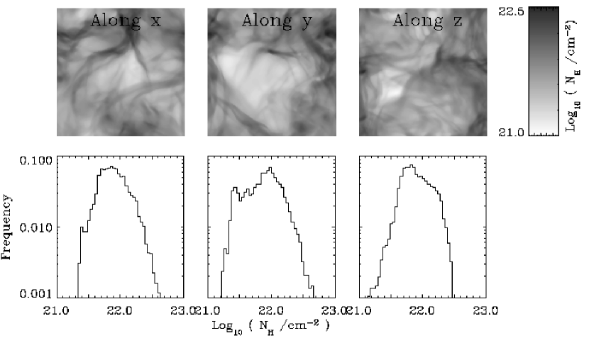
Figure 1: Surface density maps for model cloud $A$ looking along the three principal axes (top row). Histograms for the column density $N_{H}=\int n_{H}ds$ are shown (bottom row) for each viewing direction. The maps each have a mean column density $<N_{H}>=10^{22}$ cm^-2.

Our measurements begin at system time $t$ = 0.0, when the model has reached an equilibrium state between the energy dissipation rate due to shock interaction and numerical diffusion, and the driving energy input rate. The final turbulent density continuum has a density range of four orders of magnitude; two orders of magnitude above and below the mean. Surface density maps of the MHD simulation used to construct Cloud $A$ looking along the three coordinate axes are shown in Figure 1. Also shown are histograms of the column densities $N_{H}$ for the maps normalised arbitrarily to an average column of $<N_{H}>=10^{22}$cm^-2. Viewing along the B field (along $z$) reveals no strong features that distinguish it from views made perpendicularly to the B field (along $x$ and $y$). This is unsurprising, given the relatively weak magnetic field in this model.

2.2 The ISRF and dust properties

We bathe the models in the ISRF of Mathis, Mezger and Panagia (1983). Our sampling of ISRF wavelengths ($\sim 20$ distributed logarithmically in the range $[91$nm$,2\mu$m$]$) ensures that the attenuated intracloud radiation field $J_{\lambda}$ possesses an agreeably smooth spectrum when interpolated to unsampled wavelengths. One needs a more comprehensive sampling of mid-infrared wavelengths to capture the spectral features associated with the polycyclic aromatic hydrocarbons (PAHs), increasing the computational time considerably. Juvela and Padoan (2003) have addressed this problem by devising a “library method”, inferring the overall spectral form from radiative transfer calculations made at a small number of reference wavelengths. We do not consider PAHs here, since their contribution to the far-IR emission is negligible.

To illustrate the qualitative effects of the intracloud radiation field on dust grains we have constructed a grain ensemble by applying the Mathis, Rumpl & Nordsieck (1977, hereafter ‘MRN’) grain-size distribution to the graphite and astronomical silicate grains advocated in DL84. This choice of grain ensemble is meant only to illustrate possible effects. The exact nature of real interstellar dust is unknown despite being the subject of considerable study and speculation (e.g Aannestad 1975; Wright 1987; Mathis & Whiffen 1989; Smith, Sellgren & Brooke 1993). However, the DL84-MRN combination of grain composition and size distribution reproduces most aspects of the mean Galactic extinction curve (Savage & Mathis 1979).

The scattering phase function was taken to be the Henyey-Greenstein (1941) $\Phi(\omega,g)$ with the albedo, $\omega$, and $g\equiv<\cos\theta>$, the angle of scattering. Draine (2003) has proposed another scattering function, which differs from the HG function by less than 10% over the range $0.48\mu$m$<\lambda<0.96\mu$m and is presumably more realistic. We stayed with the HG function because it can be manipulated analytically with greater ease.

We calculate temperatures for grains with radii distributed logarithmically in the range $0.005\leq a\leq 0.25\mu$m. This grain size range was sampled densely enough (usually 16 different radii) to ensure that all changes in grain temperature across the range were captured. At the very smallest radii $a<0.005\mu$m transient heating may be important (Draine & Li 2001 and references therein). These very small grains must be treated outside the radiative equilibrium approximation, considering the effects of the individual photon absorption events that momentarily heat the grains to high temperatures.

3 Dilution of the Ambient Galactic Radiation Field within a Clumpy Sphere

3.1 Radiative transfer approach

We calculate the scattering within the cloud to obtain the mean specific intensity $J_{\lambda}({\bf x})$ at the point ${\bf x}$ by a Monte Carlo approach described in the Appendix, considering only wavelengths for which emission from grains is negligible. Our technique is a variant of the usual Monte Carlo method, which enables us to obtain a relatively high degree of accuracy at a respectable computational cost. Rather than compute $J_{\lambda}$ throughout the cloud by propagating photons inward from the edge, we chose a sample of interior points at which we wished to compute the radiation field, selected a sample of incoming ray directions, and propagated the rays out backwards to the cloud edge (see Lu & Hsu 2003 and references therein for a discussion of the method in the context of engineering problems). This reverse method is a computationally efficient way to calculate the mean intensity accurately at a modest but sufficient subsample of points within the model clouds. It is particularly effective when applied to self-shielded locations through which relatively few photons pass according to most other forward method Monte Carlo schemes.

3.2 Calculations with a Uniform Cloud

We establish the accuracy of our radiative transfer code by evaluating the mean intensity for the case of a uniformly dense sphere of central optical depth $<\tau_{cen}>=10$, and comparing with the semi-analytical solutions of Flannery, Roberge & Rybicki (1980). In much of what follows, we will use the uniform cloud as a standard against which to compare similarly calibrated clumpy model clouds.

For each position of interest the radiative transfer code follows rays distributed uniformly in $N$ directions. For each direction we initiate $M$ rays. In its less-than-optimal configuration ($N=16\%$ of the optimum number $N_{opt}\sim 5\times 10^{4}$ of rays, $M\sim 10$; see Appendix), the code achieves a rms error of 1.4% (see Fig. 2). The small deviation of the numerical from the analytical solution near the edge can be traced to the breakdown of the asymptotic approximation in the analytic solution which leads to an underestimation of $J/I_{0}$. We regard this degree of accuracy as acceptable; it can be improved by computing more raypaths, but requires more resources. With $N/N_{opt}=0.16$, $M=10$, $J$ may be found for $4$ $10^{4}$ points inside a 128³ cell model in about one hour on a desktop computer such as a single processor SGI or Sun workstation. All subsequent calculations use the code in this configuration unless noted otherwise.

3.3 Effects of model resolution on radiative transfer

With clumped models the geometric center of the cloud has only one unique property: at a reference wavelength ($\lambda=550$nm) we specify the average central optical depth within the cloud by computing the column density along radial paths from the center to the edge of the cloud. We force their average optical depth to be the specified value (usually 10). Every other wavelength has a mean central optical depth in proportion to the dust opacity relative to $\lambda=550$nm.

In this section we discuss only the results for $\lambda=550$nm, in which the mean central radial optical depth is 10.

A major goal is to determine the effects of clumping on the distribution of mass with $J_{550}$. For convenience in plotting, we define the mass distribution function $df_{m}/d\log_{10}(J/I_{0})$ to be the fraction of the cloud mass per unit $\log_{10}(J/I_{0})$. We also consider a similar distribution function $f_{V}$ for the volume fraction.

We first consider the effects of spatial resolution on the distribution functions. Will small, dense, dark clumps that are unresolved in coarse-grained simulations contain appreciable amounts of mass at small values of $J$? The simulation cubes are available (see Table 1) at resolutions of $512^{3}$, $256^{3}$ and $128^{3}$ cells, the highest resolution simulations possessing small scale structures that cannot be resolved by runs at the lower resolutions. These extra structures potentially provide windows through which radiation can stream, with less attenuation, increasing the mean intensity within the cloud. On the other hand, at increased resolution it is possible to form tiny, dense cores which potentially are extremely dark. It is of interest to see how the resolution of the models affects our computations of $J_{\lambda}({\bf x})$ and the distribution functions.

Models with the same input parameters but run at different resolution are actually dynamically different from each other, because the random driving pattern used to drive the turbulence will take on different realizations with varying resolution, as will the numerical diffusivities. Therefore, we compare a sequence of models derived from the 512³ model by degrading the resolution. A $512^{3}$ cell cloud may be smoothed into a $256^{3}$ cell cloud by taking a cube of eight cells and replacing them by one supercell having their average density, thereby conserving the mass. Repeated smoothings must eventually render the cloud uniform, the result of which is typically a darker cloud throughout the volume.

The effects of smoothing a cloud from 512³ to lower resolutions (256³, 128³ and 64³) are shown in Figure 3. The left panels in Figure 3 shows $J(512^{3})/J$ for various other resolutions, plotted against the densities, $n_{H}$, in the cells. The 512³ model is model C in Table 1. The coarsest (64³) resolution is in the lowest panel in the figure. As the resolution coarsens we see that the range of densities narrows, the spread in $J$ at a particular $n_{H}$ increases, and the mean $J$ decreases for all densities except those at the high end. The right panels show the changes in $J$ within individual cells brought on by coarsening the resolution. At the coarsest grid we considered (64³), the mean $J$ is not only broadened but also significantly decreased on the average because the radiation cannot easily penetrate through low-density cells since these have been eliminated by the smoothing process. Conversely, at the highest densities the smoothing process tends to increase the energy that penetrates into these regions; the dense, dark cores resolved at a resolution of 512³ are smoothed over into less dense and more penetrable regions. Overall, smoothing the model from a resolution of 512³ to 256³,128³ and 64³ cells decreases the total energy (according to a volume average) that penetrates into the cloud by approximately 1%,6% and 60% respectively.

Since the results at 512³, 256³, and 128³ are quite similar to each other, while the results at 64³ are noticeably different, it is tempting to say that the models are converging and that a resolution of 128³ is adequate for determining the distribution functions and other statistical properties of the radiation field. Quantitatively, however, the criterion for convergence is not entirely clear. Applying the fiducial optical depth of $\tau\sim 20$ across a model of resolution $\mathcal{R}$ yields a mean-free path of $\mathcal{R}/20$ cells, a size-scale resolved adequately by even the 64³ smoothed model. However, there is extreme clumping in the model (about 4 orders of magnitude) on size scales comparable to the radius of the cloud. The porosity allows radiation to penetrate deeply if the passages are spatially resolved. The 64³ resolution evidently fails to provide sufficient porosity.

4 CALCULATIONS WITH THE MODELS

4.1 Mean Intensity

In what follows we ran the Monte Carlo radiative transfer code with the model clouds, calculating the mean intensity $J_{\lambda}$ for a density weighted random sample of $8\times 10^{4}$ points. The density weighted sampling of points is akin to picking hydrogen atoms at random and asking what the ambient radiation field is like in the vicinity of that atom. Since the density ‘continuum’ is defined on a grid, we do not attempt to define $J_{\lambda}$ on smaller scales; instead we assume it is uniform within each cell. However, the radiative transfer method can in principle calculate $J_{\lambda}$ on arbitrarily small scales.

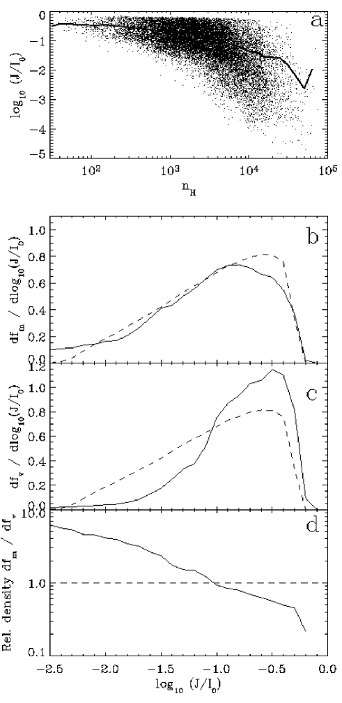
Figure 4: a The relative mean intensity $J_{550}/I_{0}$ at $\lambda=550$nm for a random sample of points within cloud $A$, where $I_{0}$ is the intensity of unattenuated interstellar radiation, assumed to be isotropic. The average $J_{550}/I_{0}$ for a given density $n_{H}$ is shown by the bold line. b The fraction of the cloud mass per unit $log_{10}($$J_{550}/I_{0}$$)$, $df_{m}/dlog_{10}($$J_{550}/I_{0}$$)$. c The equivalent volumetric distribution $df_{v}/dlog_{10}($$J_{550}/I_{0}$$)$. d The average overdensity associated with a value of $J_{550}/I_{0}$ (i.e. $df_{m}/df_{v}$).

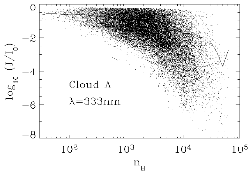
Figure 5: Like Figure 4a but calculated at $\lambda=333$nm. Note the scatter and compare the scale with Figure 4a.

Figure 4 shows various distributions that illustrate the basic statistical properties of the intracloud radiation field. The top panel (Fig. 4a) shows the scatter of $J_{550}/I_{0}$, the relative mean intensity at $\lambda=550$nm, plotted against density $n_{H}$. On average $J_{550}$ drops as $n_{H}$ increases (Fig. 4a) but the scatter about this trend is extremely large. The sharp upper limit to $J_{550}/I_{0}$ is readily identified with points lying near the cloud’s surface ($0.98<\frac{r}{R}<1.0$), illuminated by $\sim 2\pi$ steradians of almost unattenuated ISRF in addition to a small contribution that passes through the cloud. In Figures 4b and 4c we show the mass and volume distribution functions respectively. For comparison the result for the uniform cloud is also shown. The distribution of the model cloud’s mass favors lower values of $J_{550}/I_{0}$ (mass distribution peaks at $J_{550}/I_{0}$$\sim 0.1$) than in the uniform cloud, with about 16% of the cloud’s mass associated with a low intensity tail ($J_{550}/I_{0}$$<0.01$). By volume, the model cloud is brighter than the uniform cloud. These two effects result from an overall anticorrelation between $J_{550}$ and $n_{H}$, suggested in Figure 4a and shown explicitly in Figure 4d. In Figure 5 we show a plot similar to Figure 4a but evaluated at $\lambda=333$nm. It shows that at shorter wavelengths, at which the cloud is optically thicker, the scatter in $J_{\lambda}$ is generally larger.

The intracloud radiation fields at $330$nm (dashed lines) and $550$nm (solid lines) averaged in thin spherical shells of radius $r$ are shown in Figure 6. The average central optical depths are approximately 16 at 330 nm and 10 at 550nm. Compared to the uniform cloud, the mean intensity in the model cloud is enhanced dramatically, and is insensitive to radial position in the inner 50% of the cloud’s volume ($r<0.8R$), increasing rather sharply near the cloud’s outer surface ($r>0.8R$). There is also less reddening from edge to center (we discuss color in §4.2). Despite the average uniformity of $J_{550}/I_{0}$ in the cloud’s interior, it should be recalled that the scatter from point to point is large throughout (see Fig. 4a).

4.2 Intracloud Colors

The color variation inside the cloud is the result of the differential spectral extinction by the dust. The mean intensity $J_{\lambda}$ at each point inside the cloud is formed from an average over the rays propagating from the point to the surface of the cloud, each ray contributing differently to $J_{\lambda}$ by virtue of their different path histories. At some other wavelength the optical properties of the scattering dust will be different, and so too the transfer of radiation which must be recalculated for each new wavelength. As a result one might expect a scatter in colors amongst points with similar $J$ at some fixed wavelength. Possible degeneracies arise: locations of similar $J_{\lambda}$ at some wavelength may be bathed in $4\pi$ steradians of highly reddened, diffuse glow; a small but unattenuated shaft of pristine ISRF; or, most plausibly, some intermediate case.

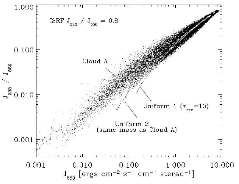
Figure 7: The color $J_{333}/J_{550}$ for points inside model $A$. For comparison the colors for two uniform clouds are shown: Uniform 1 is calibrated to $\tau_{cen}=10$ whereas Uniform 2 has a total mass equal to that of model $A$.

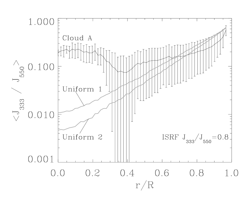
Figure 8: The color $J_{333}/J_{550}$ averaged in spherical shells centered in Cloud $A$. The averaging is density rather than volume weighted, reflecting the average color seen by an H atom or dust grain in these shells. The error bars represent the rms scatter about the mean. For comparison two uniform cloud results are shown; Uniform 1 with $<\tau_{cen}=10>$ and Uniform 2 with the same mass as model $A$.

Figure 7 illustrates the effect of clumpiness on intracloud colors; the dark locations typically see the most reddened radiation fields, but there is a spread of colors for a given $J_{550}$. In light of the anti-correlation between mean intensity $J$ and density $n_{H}$ one recovers the expected result that dense places are typically reddened. Nevertheless, over the innermost $50\%$ of the cloud’s volume the average color seen by dust grains is considerably bluer (up to a factor of $100$ for $J_{333}/J_{550}$) and less dependent on radial location than the color in uniform clouds with either the same optical depth or same mass (Fig. 8).

The color and more generally the spectral shape of the radiation field is an important factor in grain heating (see §5), and must also play a role in cloud chemistry.

4.3 Comparison between Fractal and Turbulent MHD Clouds

The turbulent cloud models used in this study were originally generated to study cloud dynamics, and were developed at considerable computational cost. As we discussed in §§2 and 3.3, they suffer from their own idealizations: finite numerical resolution and a probably unrealistic form of dynamical driving are two of them. In order to probe which features of the model are robust, and investigate whether a simpler prescription for generating density structure might give similar results, we investigated the radiation field in a hierarchical model of the gas density which is intended to replicate a fractal density distribution (Elmegreen 1997).

The fractal clouds are grown from seeds, uniquely determining the precise density structure for a given fractal dimension $D$. The clouds are grown from an initial casting of 32 points according to the seed and fractal dimension $D$. In each of the subsequent castings a further 32 points are cast about each extant point according to the fractal dimension. In a total of four castings a total of $32^{4}$ points are therefore cast, and if rendered on a $64^{3}$ cell grid the average density is $4$ points per cell. In the instances where a uniform background is desired a further $2$ points per cell are added. Finally the fractal clouds are calibrated to $<\tau_{cen}>=10$.

Figure 8 shows $df_{m}/d\log_{10}($$J_{550}/I_{0}$$)$ for both fractal and MHD models. The heavy solid line is a uniform density model. There are four types of fractals: fractal dimension 2.3 and 2.6, each containing either no uniform density background or 1/3 of the mass in such a background. For each type of fractal distribution six models were calculated, each with a different initial seed that determines the locations of the 32 points in the first casting of points. The final model contains hierarchically clumped clouds around each of the initially placed points.

The “error bars” in Figure 9 are not errors, but are the upper and lower envelope of the six individual mass distributions for the fractal dimension $D=2.6$ and no background density. The deviations of the other fractal distributions show similar deviations. The smaller ”error bars” around the light solid line shows the time variability in the MHD models.

The large scatter in the fractal results indicates that the cloud structure and radiation transport properties depend strongly upon the seed from which the cloud is grown. This scatter means that it is difficult to differentiate between fractal dimensions (either with or without uniform backgrounds) based upon their $f_{m}$ distributions. The fractal models with a background density contain a greater fraction of mass at intensities brighter than $\log_{10}($$J_{550}/I_{0}$$)=-0.5$ than do similar fractal models without a background. The addition of a background to the fractal clouds generally produces average $f_{m}$ distributions similar to those for the model clouds. Therefore, these fractal models appear to be a promising alternative testbed for studying the properties of radiation in clumpy clouds. At the same time, these results imbue the dynamical models with a pleasing degree of generality.

The relatively small characteristic scatter amongst the MHD distribution functions corresponds to the use of the different time dumps in lieu of multiple MHD clouds rendered separately but sharing the same physical parameters. This time difference is so small (about 0.2 dynamical crossing times) that the MHD models are physically correlated on large scales. Note that even with this relatively small time variation, the curves for models A and B - the former gas dominant, the latter magnetically dominant - are nearly indistinguishable.

5 GRAIN TEMPERATURES AND EMISSIVITIES IN THE MODEL CLOUDS

In Section §4 we investigated the extent to which monochromatic radiation at selected wavelengths penetrates our model clouds. The calculation of dust grain temperature is a matter of determining the spectral energy density throughout the cloud and the subsequent selective absorption and re-emission by the grains themselves. It should be emphasised that the choice of grain model has been made merely to illustrate possible grain heating effects, and that the resultant emissivities are not intended to be firm predictions.

5.1 Basic Equations. Calculating $T_{g}$

The steady state equilibrium temperature, $T_{g}$ of grains bathed by a mean intensity $J_{\lambda}$ is determined by balancing the radiative energy absorbed with that emitted thermally (see DL84),

$$\int_{0}^{\infty}Q_{abs}(a,\lambda)J_{\lambda}d\lambda=\int_{0}^{\infty}Q_{abs}(a,\lambda)B_{\lambda}(T_{g})d\lambda,$$ (1)

where $Q_{abs}(a,\lambda)$ is the absorption efficiency for a grain of radius $a$ at wavelength $\lambda$ and $B_{\lambda}(T_{g})$ is the blackbody function evaluated at the dust grain temperature $T_{g}$.

For very small grains ($a<0.01\mu$m) the steady state approximation begins to break down; individual UV photons are sufficiently energetic to heat small grains to relatively high temperatures which subsequently cool between absorption events. These transiently heated grains primarily re-radiate their energy shortward of $\lambda=100\mu$m, and may be safely excluded in this FIR analysis; for a treatment of sporadic heating of small grains in clumpy clouds see Juvela & Padoan (2003).

5.2 Results

Qualitatively, the temperature of a grain is determined by the contrast between the grain’s absorption efficiencies in the visible and FIR spectral regimes. It is often stated that small grains are hotter than large grains because they are to radiate away their energy at wavelengths much larger than their radii. In order to reach a radiative equilibrium they must attain high internal temperatures, and corresponding black-body radiation densities peaked at shorter wavelengths. This reasoning assumes that all grains absorb a similar amount of radiation per unit grain area. Since the absorption efficiency is of order unity when $a>\lambda$, this assumption is a fair approximation for large grains absorbing the ISRF. However, when the radiation field is somewhat reddened, and relatively more photons satisfy $a<\lambda$, an opposing effect comes into play. Because the grain absorption cross section reaches a maximum when $a\sim\lambda$, the reddened radiation field preferentially heats the large grains. This tends to reduce the temperature discrepancy between grains of different sizes.

The mean temperatures attained by graphite and silicate grains of various radii $a$ are shown in Table 2 for model $A$. As mentioned above, transient heating is important for the smallest grains; we include them here merely to make the point that there is now little variation in temperature with grain size. Table 2 also gives the rms variation in temperatures amongst similar grains and shows it to be a decreasing function of grain size. This occurs because of the declining importance of the highly variable blue part of the intracloud radiation field.

The fraction of the cloud’s dust mass, irrespective of grain type or size, found at temperature $T$ is shown in Figure 10. The distribution of the mass is weakly peaked at low temperatures, $T\sim 10$K with virtually all the mass contained in the MRN distribution being in the temperature range $6-17$K.

5.3 Dust Emissivity

Given a grain temperature $T_{g}$ (which generally varies from point to point and amongst grain types and sizes) the emissivity contribution $dj_{\lambda}$ from grains with radii [$a,a+da$] is given by

$$dj_{\lambda}=C_{g,s}n_{H}a^{-3.5}\times 4\pi a^{2}\times\pi B_{\lambda}(T_{g})Q_{abs}(a,\lambda)da,$$ (2)

where $B_{\lambda}(T_{g})$ is the black-body function and $Q_{abs}(a,\lambda)$ the emission efficiency.

The spectral emissivity of dust grains $dj_{\lambda}/da$ associated with a sample of randomly chosen mass is shown in Figure 11. Grains of large radii are readily identified as the principal source of the $850\mu$m emission. The smaller grains, unable to radiate away their energy at long wavelengths, dominate the emissivity at shorter wavelengths $\lambda\sim 100\mu$m.

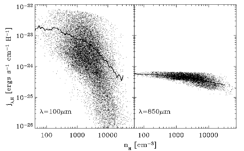
Figure 12: Specific emissivity per H atom $j_{\lambda,H}$ at $\lambda=100,850\mu$m for a random sample of atoms situated in locations of density $n_{H}$ in model $A$. The solid lines are the mean values of $j_{\lambda,H}$ associated with density $n_{H}$.

Since $850\mu$m is well into the Rayleigh-Jeans region ($hc/\lambda kT<<1$) of the spectra, the small temperature variations of the large grains responsible for this emission correspond to small variations in the $850\mu$m emissivity. On the other hand, $100\mu$m lies in the Wien spectral regime where even small temperature variations can cause large emissivity changes (Fig. 12). The small grains, sensitive to the highly variable blue part of the intracloud radiation field, find themselves with a relatively large range in temperatures. The $100\mu$m emission is therefore intrinsically more variable than the $850\mu$m emission. The $850\mu$m emissivity per H atom $j_{\lambda,H}$ varies far more slowly throughout the cloud, the volumetric emissivity $j_{\lambda}$ is then roughly proportional to density $n_{H}$.

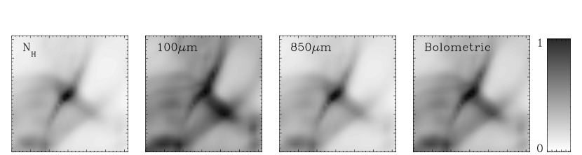
Figure 13: Surface density $N_{H}$, 100$\mu$m, 850 $\mu$m and bolometric brightness maps (left to right), scaled such that their maxima equal one.

Brightness maps (scaled so that their maxima equal 1) made by integrating the spectral emissivity $j_{\lambda}$ ($\lambda=100$ and $850\mu$m) and bolometric emissivity $j_{bol}$ through the cloud, $I_{\lambda}\propto\int j_{\lambda,H}n_{H}dx$, are shown alongside the surface density in Figure 13. The maps were made for a central cubical region ($32^{3}$ cells), looking along the $x$ axis. Since the central parts of the cloud possess a radiation field insensitive to radial location (see Fig. 7), the maps show few of the ’edge effects’ that result from a close proximity to the imposed spherical cloud surface. Instead, we primarily observe the effects of clumpiness. One can see that the brightness map at $850\mu$m corresponds best with the surface density map $N_{H}$.

Our results have bearing on the problem of directly determining the dust mass corresponding to a FIR/sub mm flux measurement. This problem has received some study, inspiring a number of different approaches (Hildebrand 1983, Xie et al. 1993; Hobson & Padman 1994; Li, Goldsmith & Xie 1999; Xie, Goldsmith & Zhou 1991). The large scatter in emissivity per H atom at 100 $\mu$m, and the relatively small scatter at 850 $\mu$m, further suggests that inferring column densities from FIR emission is best done using observations at longer wavelengths.

6 SUMMARY AND DISCUSSION

We have studied the attenuation of the interstellar radiation field by dust in models of clumpy clouds and calculated the dust temperatures and far-IR emissivities. The main conclusions are as follows:

1. Inhomogeneity of the density continuum dramatically increases the radiant energy that penetrates into the cloud, making the volume markedly brighter when compared to a uniform cloud of comparable optical depth (Fig. 4c). The mass contained in clumpy structures provides enough local attenuation that most of the mass is in fact associated with lower intensities (Fig. 4b) when compared to the uniform cloud.

2. The above two effects imply an anti-correlation of average $J$ with $n_{H}$, but from point to point there exists an extremely large scatter about this trend, more so at wavelengths at which the cloud is optically thick (Figs. 4a and 5). Despite this large scatter, the mean intensity averaged by spherical shells is largely independent of radial position within the inner 50% of the cloud volume (Fig. 6).

3. The cloud’s inhomogeneity allows small amounts of weakly unattenuated blue ISRF to penetrate the cloud which, when combined with the predominant reddened field, makes the intracloud field somewhat bluer than in the uniform cloud. The variability of this effect introduces a scatter in the color (Fig. 7) which in accordance with $J$ is also on average quite uniform throughout the model (Fig. 8).

4. The differential mass per intensity distribution of the MHD models can be qualitatively reproduced by fractal clouds generated according to a simple prescription and augmented by a uniform density background. In both types of inhomogeneous model, the peak of the mass distribution is shifted occurs at lower intensity than in a uniform cloud, suggesting that this is a robust feature of clumpiness (Figure 9). These results are relatively insensitive to fractal dimension or magnetic fieldstrength over the range explored ($D$ = 2.3 - 2.6; $\beta$ = 0.05 - 4.04).

5. For one grain model (DL84) bathed in the attenuated ISRF, the sensitivity of dust grains of different radii to the overall spectral form (i.e color) of the intracloud radiation field $J_{\lambda}$ produces average grain temperatures which do not depend strongly on the grain size (Table 2). Importantly, the smaller grains, absorbing the most variable part of the intracloud radiation field, exhibit a greater scatter in their temperatures. When considering how the dust mass is distributed with temperature there is a slight preponderance for low temperature ($T\sim 10$K) material (Fig. 10), primarily due to the abundance of silicates in the DL84-MRN grain ensemble.

6. Small, relatively hot grains emit the majority of the $100\mu$m emission, larger grains emitting longward of this (Fig. 11). The temperature variations in these two grain populations, considered in the context of the Rayleigh-Jeans and Wien spectral regimes, yield emissivities $j_{\lambda,H}$ exhibiting very different point to point variations, shown in Figure 12. The $850\mu$m emissivity per H atom varies by less than a factor of 5 whereas the $100\mu$m emissivity per H atom varies by several orders of magnitude.

7. In constructing brightness maps (Fig. 13) the intrinsic scatter in $j_{\lambda,H}$, the emissivity per H atom, that ultimately arises from the cloud’s inhomogeneity increasingly decorrelates maps made at $\lambda<100\mu$m when compared with the surface density. Conversely, maps made at longer wavelengths show increasingly higher correlations between brightness and surface density maps, and should be preferred if one wishes to infer surface densities and cloud masses from brightness maps.

.1 MONTE CARLO METHOD

We consider the trajectories of individual photons, each carrying a weight $W$. The weight reflects the probability of the photon surviving the course of its trajectory without being absorbed (e.g Witt 1977). The Monte Carlo aspect of the code deals exclusively with the scattering processes, that is, in selecting a probabilistically weighted sample of possible trajectories that connect a point within the cloud to points on the cloud’s surface. It is along such a trajectory that the weight is calculated,

$$W=exp(-\tau_{a}^{tot})$$ (1)

where $\tau_{a}^{tot}$ is the total absorption optical depth along the trajectory. The generation of trajectories and their respective weights is sufficient to evaluate the mean intensity. To explore the possible trajectories which connect a particular location inside the cloud to the external radiation field we have implemented the following reverse approach for generating photon trajectories;

An observer is placed at point A inside the cloud (Fig. 14) insisting upon knowing the intensity in $N$ directions ${\bf\hat{k}_{obs}}$ uniformly distributed over the $4\pi$ steradians of sky. For each of these $N$ directions ${\bf\hat{k}_{obs}}$ we initiate $M$ reverse trajectories.

Proceeding one trajectory at a time the free path between scattering centres, $\bf{x_{i}}$, is found from probabilistically sampling the possible optical depths $\tau_{s}$ to the next scattering event. The cumulative probability $p$ of a photon advancing $\tau_{s}$ before scattering is

$$p=exp[-\tau_{s}].$$ (2)

Rearranging yields

$$\tau_{s}=-ln(p),$$ (3)

where random numbers $p$ sampled uniformly in the interval [0,1] will correctly reproduce the distribution function (Eq. 2). The random number generator RAN2 (Press et al. 1992) is used to provide a value $p$ which then gives $\tau_{s}$ using equation (3). The free path in real space is found by evaluating $\tau^{{}^{\prime}}_{s}=\sum\sigma_{s}(\lambda)n_{H}\Delta l$ in a stepwise fashion through the cloud until $\tau^{{}^{\prime}}_{s}$ approaches $\tau_{s}$ to within an acceptable error margin.

The trajectory is updated. The free path vector to the next scattering centre is ${\bf l}=\sum\Delta{\bf l_{i}}$ and the optical depth to pure absorption $\tau_{a}=(\omega^{-1}-1)\tau_{s}$ where $\omega$ is the grain albedo. The total optical depth to pure absorption calculated along the trajectory thus far, $\tau_{a}^{tot}$, is incremented by the amount $\tau_{a}$.

The photon has now reached the location of a new scattering event. To find the direction ${\bf\hat{k}_{i}}$ in which the trajectory proceeds, one randomly samples the scattering phase function $\Phi(\theta)$. The scattering process is direction independent - the reverse scattering process is exactly the same as the forwards process. For $\Phi(\theta)$ we chose to use the Henyey-Greenstein (HG) phase function (Henyey & Greenstein 1941);

$$\Phi(\theta)=\frac{1}{4\pi}(1-g^{2})/[(1+g^{2}-2g\cos\theta)]^{\frac{3}{2}}.$$ (4)

where $\theta$ is the trajectory’s deflection (polar) angle and the asymmetry parameter $g=<\cos\theta>$ which takes a value between -1 (backwards scattering) and +1 (forwards scattering). The HG phase function is acceptably accurate ($<10\%$ error) in the range $0.48\mu$m$<\lambda<0.96\mu$m (for the DL84 grains) and can be manipulated analytically with relative ease. Typical values of g for the interstellar dust from DL84 fall in the range g$\sim 0.15$ in the NIR and g$\sim 0.65$ in the NUV.

Integrating to obtain the cumulative probability function for equation (4) and inverting the result yields $\theta(p)$,

$$\theta(p)=\frac{(1+g^{2})-[(1-g^{2})/(1-g+2gp)]^{2}}{2g}.$$ (5)

As before, $p$ is a random number uniformly distributed in the range $[0,1]$. Finally, the azimuthal deflection angle is given by $\phi=2\pi p$ where $p$ is another random number. Application of the Euler transformations on the pre-scatter direction ${\bf k_{i}}$ and deflection angles $(\theta,\phi)$ yields the new direction ${\bf k_{i+1}}$.

The scattering process is repeated until the trajectory meets the cloud surface (point B).

For a given ${\bf\hat{k}_{obs}}$ the above process is repeated $M$ times to sample the possible trajectories that intercept the observer along this direction. A new direction ${\bf\hat{k}_{obs}}$ is set and the process repeated until $NM$ trajectories have been generated with weights $W_{nm}$.

The mean relative intensity at A is then

$$\frac{J({\bf A})}{I_{0}}=\frac{1}{N}\sum_{n}^{N}\frac{I({\bf\hat{k}_{obs}},{\bf A})}{I_{0}}=\frac{1}{NM}\sum_{n}^{N}\sum_{m}^{M}W_{nm}.$$ (6)

The number $N$ of directions is set by the resolution $\mathcal{R}$ of the model cloud - the optimum $N$ is of the order $\mathcal{R}^{2}$; adjacent rays propagating in straight lines never separating by more than a cell’s width. In practise 16% of this optimum number of directions is sufficient to obtain similar results (within 3%) whilst dramatically reducing the runtime of the calculation. The number $M$ of samplings of each direction is mainly determined by the cloud’s optical properties, $M\sim 10$ being sufficient to obtain satisfactory convergence of the results (within 3% of those with $M=100$).

Figure 2: The relative mean intensity $J/I_{0}$ computed with the code (crosses) at radial positions $0<r<R$ inside a uniform cloud of central optical depth $\tau=20$ and radius $R$. The solid line is given by the closed-form asymptotic solution for optically thick clouds derived in Flannery, Roberge & Rybicki (1980).

Figure 3: Comparison of mean intensity at equivalent points (i.e cell coordinates $(x,y,z)$ in the 512³ cell model become $(x/2,y/2,z/2)$ after smoothing to 256³ cells) in model $C$ smoothed from 512³ to 256³,128³ and 64³ cells.

Figure 6: For $\lambda=333$nm (dashed line) and $\lambda=550$nm (solid line) the mean specific intensity is averaged over the volume of thin spherical shells to form the shell average $<J_{\lambda}>$. The shells are centered on the cloud center, of radii $0<r<R$ and thickness $R/50$, where $R$ is the cloud radius. Results for the uniform cloud with the same central optical depth ($<\tau_{cen}>=10$) are shown for comparison.

Figure 9: Comparison between, uniform, fractal (dimension D, with and without backgrounds ‘b.g’) and model clouds $A$ and $B$. In the case of the fractal clouds average results have been shown with standard deviations (large error bars), generated by averaging f_m for a number of clouds with the same physical parameters but grown from different seeds. The model clouds’ results are time averages during their steady-state phases (during which there are three time dumps); the deviations (small error bars) are then to be interpreted as intrinsic time variations rather than the differences between clouds sharing the same physical parameters but realised separately.

Figure 10: The mass distribution function for Cloud $A$ (solid line), such that $\int(df_{m}/dT)dT=1$. The mass includes graphite and silicate grains that fall within the MRN size range $[0.005\mu$m$,0.25\mu$m$]$. The separate contributions of the graphite and silicate grains are shown by the dashed and dot-dashed lines respectively.

Figure 11: The differential contribution $dj_{\lambda}/da$ of grains of different radii to the spectral emissivity $j_{\lambda}$ at $\lambda=100,350$ and $850$ $\mu$m (top to bottom). Each line represents the emissivity of dust associated with a randomly chosen H atom except the dashed line which is the emissivity associated with an H atom exposed to the unattenuated ISRF (i.e. an upper limit).

Figure 14: The spherical cloud sits snugly inside the cubic domain of $R^{3}$ cells. An observer A sends out $M$ rays (one of which is shown) for each of the $N$ directions (${\bf\hat{k}_{obs}}$) sampling the observe’s entire sky. Each ray is evolved according to the Monte Carlo sampling of free paths between scatterings and scattering angles until it reaches the cloud’s edge (B). The dashed lines are other trajectories joining the observer A of photons ($h\nu$) to the ISRF.

Table 1: Model list

Name	Resolution	$\beta$	Source
$A$	$128^{3}$	$4.04$	Heitsch, Mac Low & Klessen (2001)
$B$	$128^{3}$	$0.05$	Heitsch et al (2001)
$C$	$512^{3}$	$4.04$	Li, Norman & Mac Low (2004)

Note. — The MHD simulations used to make Clouds A,B and C. The parameter $\beta=P_{th}/P_{mag}=8\pi c_{s}^{2}\rho/B^{2}$.

Table 2: Average Grain Temperatures T and r.m.s scatter $\sigma$

		Log${}_{10}(a/\mu$m$)$
		-3.0	-2.0	-1.0	0.0
Graphite	T (K)	12.4	13.1	14.5	10.12
	$\sigma$	2.1	2.2	1.9	1.1
Silicate	T (K)	9.5	9.6	9.8	10.2
	$\sigma$	1.8	1.9	1.6	1.1

References

- (1)
- (2) Aannestad, P.A. 1975, ApJ, 200, 30
- (3)
- (4) Chandrasekhar, S., & Münch, G. 1950, ApJ, 112, 380
- (5)
- (6) Draine, B. T. 2003, ApJ, 598, 1017
- (7)
- (8) Draine, B. T., & Lee, H. M. 1984, ApJ, 285, 89
- (9)
- (10) Draine, B. T., & Li, A. 2001, ApJ, 551, 807
- (11)
- (12) Elmegreen, B. G. 1997, ApJ, 477, 196
- (13)
- (14) Flannery, B. P., Roberge, W., & Rybicki, G. B. 1980, ApJ, 236, 598
- (15)
- (16) Gordon, K. D., Misselt, K. A., Witt, A. N., & Clayton, G. C. 2001, ApJ, 551, 269
- (17)
- (18) Heitsch, F., Mac Low, M.-M., & Klessen, R.S. 2001, ApJ, 547, 280
- (19)
- (20) Heitsch, F., Zweibel, E. G., Mac Low, M.-M., Li, P., & Norman, M. L. 2001, ApJ, 561, 800
- (21)
- (22) Henyey, L. G., & Greenstein, J. L. 1941, ApJ, 93, 70
- (23)
- (24) Hildebrand, R. H. 1983, Q. Jl R. astr. Soc., 24, 267
- (25)
- (26) Hobson, M. P., & Padman, R. 1994, MNRAS, 266, 752
- (27)
- (28) Juvela, M., & Padoan, P. 2003, A&A, 397, 201
- (29)
- (30) Krolik, J. H. 1998, Active Galactic Nuclei: From the Central Black Hole to the Galactic Environment (Princeton, NJ: PUP)
- (31)
- (32) Li, D., Goldsmith, P. F., & Xie, T. 1999, ApJ, 522, 897
- (33)
- (34) Li, P.S., Norman, M.-L., Mac Low, M.-M., & Heitsch, F. 2004, ApJ, in press
- (35)
- (36) Lu, X., & Hsu, P.-f. 2003, in ASME 2003 Int. Mechanical Engineering Congress of IMECE,
- (37)
- (38) Mac Low, M.-M. 1999, ApJ, 524, 169
- (39)
- (40) Mathis, J. S., Rumpl, W., & Nordsieck, K. H. 1977, ApJ, 217, 425
- (41)
- (42) Mathis, J. S., Mezger, P. G., & Panagia, N. 1983, A&A, 128, 212
- (43)
- (44) Mathis, J. S, & Whiffen, G. 1989, ApJ, 341, 808
- (45)
- (46) Morris, M., & Serabyn, E. 1996, ARA&A, 34, 645
- (47)
- (48) Natta, A., Palla, F., Panagia, N., & Preite-Martinez, A. 1981, A & A, 99, 289
- (49)
- (50) Padoan, P., & Nordlund, A. 1999, ApJ, 526, 279
- (51)
- (52) Press, W. H., Teukolsky, S. A., Vetterling, W. T., & Flannery, B. P. 1992, Numerical Recipes in C (Cambridge:CUP)
- (53)
- (54) Savage, B. D., & Mathis, J. S. 1979, ARA&A, 17,73
- (55)
- (56) Smith, R. G., Sellgren, K., & Brooke, T. Y. 1993, MNRAS, 263, 749
- (57)
- (58) Spitzer, L. 1978, Physical Processes in the Interstellar Medium (New York, NY:Wiley)
- (59)
- (60) Tielens, A. G. G. M., & Hollenbach, D. 1985, ApJ, 291, 722
- (61)
- (62) Witt, A. N. 1977, ApJS, 35, 1
- (63)
- (64) Witt, A. N. & Gordon K. D. 2000, ApJ, 533, 236
- (65)
- (66) Wolf, S., Henning, T., & Stecklum, B. 1999, A&A, 349, 839
- (67)
- (68) Wright, E. L. 1987, ApJ, 320 818
- (69)
- (70) Xie, T., Goldmsith, P., Snell, R., & Zhou, W. 1993, ApJ, 402, 216
- (71)
- (72) Xie, T., Goldmsith, P., & Zhou, W. 1991, ApJ, 371, L81
- (73)