The Hot and Cold Spots in the Wilkinson Microwave Anisotropy Probe Data are Not Hot and Cold Enough

Abstract

This Letter presents a frequentist analysis of the hot and cold spots of the cosmic microwave background data collected by the Wilkinson Microwave Anisotropy Probe (WMAP). We compare the WMAP temperature statistics of extrema (number of extrema, mean excursion, variance, skewness and kurtosis of the excursion) to Monte Carlo simulations. We find that on average, the local maxima (high temperatures in the anisotropy) are too cold and the local minima are too warm. In order to quantify this claim we describe a two-sided statistical hypothesis test which we advocate for other investigations of the Gaussianity hypothesis. Using this test we reject the isotropic Gaussian hypothesis at more than 99% confidence in a well-defined way. Our claims are based only on regions that are outside the most conservative WMAP foreground mask. We perform our test separately on maxima and minima, and on the north and south ecliptic and Galactic hemispheres and reject Gaussianity at above 95% confidence for almost all tests of the mean excursions. The same test also shows the variance of the maxima and minima to be low in the ecliptic north (99% confidence) but consistent in the south; this effect is not as pronounced in the Galactic north and south hemispheres.

1. Introduction

The Wilkinson Microwave Anisotropy Probe (WMAP) data provide the most detailed data on the full sky cosmic microwave background (CMB) to date. This information about the initial density fluctuations in the universe allows us to test the cosmological standard model at unprecedented levels of detail. (Bennett et al. 2003a) A question of fundamental importance to our understanding of the origins of these primordial seed perturbations is whether the CMB radiation is really an isotropic and Gaussian random field, as generic inflationary theories predict (Starobinsky 1982; Guth & Pi 1982; Bardeen et al. 1983).

A natural way to study the CMB is to look at the local extrema. This was initially suggested because the high signal-to-noise ratio at the hot spots means they would be detected first (Sazhin 1985; Zabotin & Naselsky 1985; Vittorio & Juszkiewicz 1987; Bond & Efstathiou 1987). Heavens & Sheth calculate analytically the two-point correlation function of the local extrema (Heavens & Sheth 1999). In addition, extrema trace the topological properties of the temperature map; this makes them good candidates for study (Wandelt et al. 1998).

We pursue this investigation by simulating Gaussian Monte Carlo CMB skies and comparing the WMAP data to those simulations. We choose several statistics and then check to see if the WMAP statistics lie in the middle of the Monte Carlo distributions of statistics. We present results on the one-point functions of the local extrema: their number, mean excursion, and variance, and skewness and kurtosis of the excursion.

The literature contains many other searches for non-Gaussianity, in the WMAP data and other CMB experiments. For example, Vielva et al. detect non-Gaussianity in the three- and four-point wavelet moments (Vielva et al. 2004), Chiang et al. detect it in phase correlations between spherical harmonic coefficients (Chiang et al. 2003; see also Chiang et al. 2002, 2004), and Park finds it in the genus Minkowski functional (Park 2004). Eriksen et al. find anisotropy in the $n$-point functions of the CMB in different patches of the sky (Eriksen et al. 2004). Others discuss possible methods of detecting non-Gaussianity. Aliaga et al. look at studying non-Gaussianity through spherical wavelets and “smooth tests of goodness-of-fit” (Aliaga et al. 2003). Cabella et al. review three methods of studying non-Gaussianity: through Minkowski functionals, spherical wavelets, and the spherical harmonics (Cabella et al. 2004). They propose a way to combine these methods.

Komatsu et al. discuss a fast way to test the bispectrum for primordial non-Gaussianity in the CMB (Komatsu 2003a), and do not detect it (Komatsu et al. 2003b). Finally, Gaztañaga et al. find the CMB to be consistent with Gaussianity when considering the two and three-point functions (Gaztañaga & Wagg 2003; Gaztañaga et al. 2003). To this work, we add a strong detection of non-Gaussianity based on generic features: the local extrema.

The Letter is laid out as follows. The next section discusses our method for making Monte Carlo simulations of the CMB sky and calculating statistics on both the simulations and the WMAP data. It also explains our statistical tests. Section 3 describes our results. We conclude in section 4.

2. Method

We test the WMAP data of the CMB sky by comparing the one-point statistics of its extrema to those same statistics on several sets of Monte Carlo–simulated Gaussian skies. Our null hypothesis is that the statistics of the WMAP data are drawn from the same probability density function (PDF) as the statistics of the Monte Carlo skies. If some WMAP one-point statistic falls lower or higher than most of the Monte Carlo statistics, this indicates that our hypothesis may be false.

We examine several inputs to our Monte Carlo simulation to see how those change the Monte Carlo distribution of one-point statistics around the WMAP one-point statistics. We start very generally, looking at different frequency bands and Galactic masks, and then narrow our search. Initially, we look at simulations including the three frequency bands (Q, V, and W) and the three published Galactic masks for the WMAP data. Then we check to see if changing to a different published theoretical power spectrum affects our results. Finally, we look for anisotropy between the statistics of the ecliptic and Galactic north and south hemispheres.

2.1. Monte Carlo Simulation

A general outline of our Monte Carlo simulation process follows. Each set of skies is labeled by its theoretical power spectrum, frequency band (Q, V, or W), and Galactic mask. The frequency band determines both the (azimuthally averaged) beam shape function and the noise properties on the sky. The simulated CMB skies are created as follows:

1. A Gaussian CMB sky is created with SYNFAST, using a power spectrum and a beam function. The HEALPix pixelization of the sphere is used, with $N_{side}$ = 512.

2. Random Gaussian noise is added to the sky (at each pixel) according to the published noise characteristics of the band being simulated. The WMAP radiometers are characterized as having white Gaussian noise (Jarosik et al. 2003).

3. The monopole and dipole moments of the sky (outside of the chosen Galactic mask) are removed.

We make no attempt to simulate any foregrounds, including the galaxy; our analysis ignores data inside a Galactic mask and uses the cleaned maps published on LAMBDA (Legacy Archive for Microwave Background Data Analysis; NASA 2003).

For each Monte Carlo set, one of four power spectra is used. These are the power spectra published by the WMAP team on LAMBDA (NASA 2003). We primarily use the best-fit (bf) theoretical power spectrum to a cold dark matter universe with a running spectral index using the WMAP, Cosmic Background Imager (CBI), Arcminute Cosmology Bolometer Array Receiver (ACBAR), Two-Degree Field, and Ly$\alpha$ data. In addition, we check the unbinned power spectrum (w) directly measured by WMAP, the power law (pl) theoretical power spectrum fit to WMAP, CBI and ACBAR, and a running index (ri) theoretical power spectrum fit to WMAP, CBI and ACBAR. See Spergel et al. (2003), Bennett et al. (2003a), and NASA (2003) for more information.

The Galactic masks used are the Kp0, Kp2, and Kp12 masks published by the WMAP team (Bennett et al. 2003b). To check for differences between the north and south ecliptic hemispheres, we define additional masks that extend the Kp0 Galactic mask to block either the north or south hemisphere as well. For example, the ecliptic south (ES) mask blocks the northern ecliptic sky as well as the galaxy. As a control, we also extend the Kp0 mask for Galactic north and south hemispheres (GN and GS) to bring the total number of masks up to seven: Kp0, Kp2, Kp12, GS, GN, ES, EN. We use the same masking and dipole removal procedure for the WMAP data as for the Monte Carlo skies.

The WMAP data that we use are the cleaned, published maps. They are published by channel, so we calculate an unweighted average over (for example) all four W-band channels to get a map for the W band. The noise variance is calculated accordingly. We compute an unweighted average of the maps so that we can combine the WMAP beam functions through a simple average.

2.2. Analysis and Hypothesis Test

Our analysis of both the Monte Carlo and WMAP skies involves the following: We find the local maxima and minima of the HEALPix grid using HOTSPOT. Then we discard the extrema blocked by the Galactic mask. We calculate the statistics (number, mean, variance, skewness, and kurtosis) on the temperatures of the maxima and minima, and then statistically analyze the significance of the position of the WMAP statistic among the Monte Carlo statistics. Because we consider only the one-point statistics, we consider only the temperature values, not their locations.

We calculate our five statistics for the maxima and minima separately. The two statistics which are typically negative for the minima, the mean and skewness, are multiplied by $-1$ in our results, to make comparison with the maxima statistics more clear.

For the rest of this section, we explain our analysis of the statistics in detail. To simplify the discussion, we consider the analysis of only one statistic on either maxima or minima, as we analyze the results for each statistic separately.

Our Monte Carlo simulations are binomial trials, where the statistic calculated on a simulation can lie either above or below the WMAP statistic. It lies below the WMAP statistic with probability $p$, and for some set of $n$ trials, $i$ of the trials will have statistics below the WMAP statistic. Given $p$, the probability of $i$ is $P(i|p)=[n!/i!(n-i)!]p^{i}(1-p)^{n-i}$. The value $\hat{p}\equiv i/n$ is both an unbiased and maximum likelihood estimator of $p$.

We are interested in whether $p$ is near 0 or 1, since that indicates that our hypothesis—that the WMAP statistic came from the same PDF as the Monte Carlo statistics—may be false. Because we do not have an alternative distribution for the WMAP statistic that we can test against the Monte Carlo distribution, we do not test our hypothesis as phrased. We only look at a hypothesis $H_{0}$ that claims $p$ is in some interval, $p\in(\alpha/2,1-\alpha/2)$, where we have arbitrarily chosen $\alpha=0.05$.

We devise a statistical test of this hypothesis. Given our experimental result $i$, we construct the $1-\alpha=95\%$ symmetric confidence interval for $p$, as described in Kendall & Stuart (1973). If this confidence interval lies entirely within the interval $[0,\alpha/2]$ or entirely within $[1-\alpha/2,1]$ then we reject our hypothesis, $H_{0}$. We reject $H_{0}$ for no values of $i$ when $n=99$, for $0\leq i\leq 15$ or $985\leq i\leq 1000$ when $n=1000$, and for $0\leq i\leq 103$ or $4897\leq i\leq 5000$ when $n=5000$.

This interval is a “95%” confidence interval in the following frequentist (non-Bayesian) sense. Suppose we repeat the experiment (with the same number of Monte Carlo runs, and the same WMAP data) many times and get many values of $i$. We recalculate the confidence intervals each time, for each particular value of $i$. Ninety-five percent of the confidence intervals we calculate will contain the true value of $p$.

Our test is biased in favor of $H_{0}$. Let $H_{1}$ be the alternative hypothesis $p\in[0,\alpha/2]\cup[1-\alpha/2,1]$. Then, for some values of $p$ where $H_{1}$ is true (for example, $p=0.02$, $n=1000$), our test will choose $H_{0}$ more often than $H_{1}$, given that $i$ is a random variable with probability $P(i|p)$. If desired, we can make the test unbiased by changing our value of $\alpha$ in the hypotheses $H_{0}$ and $H_{1}$, but keeping the test (range of $i$ for which $H_{0}$ is accepted) the same.

For $n=1000$, we have an unbiased test if $\alpha=0.0313$, and for $n=5000$, we have an unbiased test if $\alpha=0.0415$. Note that these values are less than $\alpha=0.05$. For any value of $p$, these tests are at least as likely to choose the correct hypothesis as the incorrect one. This is a 50% confidence, as opposed to our previous 95% confidence. This interpretation of the test does not change our results; it merely provides the different perspective that our test may be considered an unbiased 96.9% test, for $n=1000$; or an unbiased 95.9% test, for $n=5000$.

3. Results

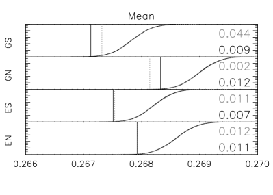
Figure 1.— Cumulative distribution functions (CDFs) of mean temperature value (in units of millikelvins) of the local extrema, found in sets of 5000 Monte Carlo simulations for four Galactic masks: GS, GN, ES, and EN. Best fit power spectrum and W-band data are used. Means of the minima are negated for comparison. Maxima CDF is dotted while minima CDF is solid. Note their visual similarity. Statistics measured on WMAP data are shown as two vertical lines, dotted for maxima and solid for minima. Numbers on right are the same probabilities as in Table 3; for each pair, probability for the maxima is higher on the page.

Table 1Estimated Probabilities $\hat{p}$ of the CMB Statistics Being Less than the Value Measured by WMAP, Based on Several Monte Carlo Samplings of Those Statistics

Identifier	0	1	2	3	4	5
bf, Q, Kp0, max	0.374	0.000	0.030	0.566	0.889	99
bf, Q, Kp0, min	0.010	0.000	0.232	0.919	0.707
bf, Q, Kp2, max	0.333	0.000	0.152	0.545	0.899	99
bf, Q, Kp2, min	0.010	0.000	0.293	0.919	0.768
bf, Q, Kp12, max	0.020	0.000	0.576	0.929	1.000	99
bf, Q, Kp12, min	0.000	0.000	0.798	0.919	1.000
bf, V, Kp0, max	0.091	0.616	0.182	0.495	0.848	99
bf, V, Kp0, min	0.030	0.182	0.303	0.990	0.960
bf, V, Kp2, max	0.061	0.384	0.061	0.364	0.727	99
bf, V, Kp2, min	0.040	0.202	0.263	1.000	0.960
bf, V, Kp12, max	0.000	0.384	0.212	0.343	0.889	99
bf, V, Kp12, min	0.020	0.232	0.444	0.980	1.000
bf, W, Kp0, max	0.475	0.000	0.141	0.364	0.475	99
bf, W, Kp0, min	0.414	0.000	0.343	0.879	0.646
bf, W, Kp2, max	0.495	0.000	0.131	0.182	0.283	99
bf, W, Kp2, min	0.293	0.000	0.323	0.808	0.616
bf, W, Kp12, max	0.434	0.000	0.242	0.313	0.253	99
bf, W, Kp12, min	0.364	0.010	0.505	0.707	0.737
pl, W, Kp0, max	0.427	0.002*	0.129	0.461	0.410	1000
pl, W, Kp0, min	0.377	0.000*	0.224	0.880	0.704
ri, W, Kp0, max	0.388	0.000*	0.216	0.285	0.310	1000
ri, W, Kp0, min	0.396	0.000*	0.406	0.821	0.618
w, W, GS, max	0.633	0.023	0.362	0.045	0.304	1000
w, W, GS, min	0.685	0.007*	0.981	0.247	0.213
w, W, GN, max	0.436	0.000*	0.168	0.504	0.159	1000
w, W, GN, min	0.243	0.006*	0.060	0.832	0.610
w, W, ES, max	0.607	0.010*	0.869	0.103	0.429	1000
w, W, ES, min	0.176	0.003*	0.923	0.244	0.152
w, W, EN, max	0.470	0.011*	0.019	0.416	0.119	1000
w, W, EN, min	0.702	0.005*	0.067	0.958	0.861
bf, W, GS, max	0.603	0.044	0.240	0.152	0.434	5000
bf, W, GS, min	0.641	0.009*	0.852	0.405	0.284
bf, W, GN, max	0.371	0.002*	0.091	0.648	0.284	5000
bf, W, GN, min	0.209	0.012*	0.035	0.883	0.697
bf, W, ES, max	0.560	0.011*	0.472	0.198	0.487	5000
bf, W, ES, min	0.151	0.007*	0.586	0.376	0.253
bf, W, EN, max	0.436	0.012*	0.002*	0.529	0.188	5000
bf, W, EN, min	0.668	0.011*	0.011*	0.960	0.869