Survival Rates and Consequences

Abstract

To first order, the initial cluster luminosity function appears to be universal. This means that the brightest young cluster in a galaxy can be predicted from the total number of young clusters based purely on statistics. This suggests that the physical processes responsible for the formation of clusters are similar in a wide variety of galaxies, from mergers to quiescent spirals. One possibility is that conditions for making young massive clusters are globally present in mergers while only locally present in spirals (i.e., in the spiral arms). However, understanding the destruction of clusters and the accompanying survival rates is more important for understanding cluster demographics than understanding their formation. This is because only about 1 in 1,000 clusters with mass greater than 10⁴ M_⊙ will survive to become an old globular cluster. In this paper we briefly review this basic framework and then develop a toy model that allows us to begin to address several fundamental questions. In particular, we demonstrate that young clusters in the Antennae Galaxies have a high “infant mortality” rate, with roughly 90 % of the clusters being destroyed each decade of log(time). We also advocate the use of an objective classification system for clusters, with the three parameters being mass, age, and size.

Space Telescope Science Institute, 3700 San Martin Dr., Baltimore, MD, 21218, USA

1. Introduction

Historically, star clusters have been divided into three types in the Milky Way; globular clusters, open clusters, and associations. This has conditioned us to think in terms of three distinct modes of cluster formation. However, when we look at external galaxies we see a power law continuum of young cluster masses. How can these two outlooks be reconciled?

There is growing evidence that all star clusters may form from a universal initial cluster mass function, which is then modified by a variety of destruction mechanisms. These destruction mechanisms include infant mortality (e.g., unbound clusters that freely expand in the first $\approx$ 10 Myr), environmental effects (e.g., disk and bulge shocking, dynamical friction), internal effects (e.g., evaporation from 2-body relaxation ) and stellar evolution (e.g., mass loss). By convolving these formation and destruction rates with the star formation history of a galaxy, and after taking into effect various observational artifacts and selection effects, we should be able to predict the current distribution of young and old star clusters we see in a particular galaxy.

In this contribution we first outline some of the results which have lead to the development of this basic framework, and then develop a “toy” model designed to help answer three fundamental questions.

1.1. Is the Initial Cluster Mass Function Continuous or Modal ?

Essentially all studies of the luminosity functions of young clusters have found them to be power laws, $\phi(L)dL\propto L^{\alpha}dL$ with a value of $\alpha$ $\approx$ –2 (e.g., Whitmore et al. 1999, see Whitmore 2003 for a review [originally appearing in 2000 as astro-ph/0012546]). Mass functions have been determined for only a small subset of these galaxies, but a similar power law relationship is generally found, again with an index –2 (e.g., Zhang and Fall 1999). On the other hand, the luminosity and mass functions of old globular clusters are peaked, with a mean $V$ magnitude M_v $\approx$ -7.4, a mean mass $\approx$ 2 $\times$ 10⁵ M_⊙, and a width $\sigma\approx 1.4$ mag (e.g., Whitmore 2003). Several theoretical studies (e.g., Vesperini 1998, Fall and Zhang 2001) have suggested that a natural way to explain this apparent discrepancy is the destruction of the fainter, less massive clusters, due to effects such as 2-body relaxation, tidal shocks, and stellar mass loss.

Other theoretical studies have also highlighted the important role that cluster destruction may play in determining the demographics of clusters (e.g., Fall & Rees 1977, Gnedin & Ostriker 1997). The current paper adopts a similar framework, but broadens it to include all star clusters; young and old, near and far. The basic question is: “Can all observations of star cluster demographics be explained by a universal initial cluster mass function followed by the destruction of a subset of the clusters which carves away regions of parameter space ?”

1.2. Is the Initial Cluster Mass Function Universal ?

On the surface, the demographics of star clusters appear to differ dramatically in different galaxies. For example, merging galaxies have large numbers of very bright, very massive young clusters, often called super star clusters. On the other hand, in relatively quiescent galaxies, such as the Milky Way, the young clusters appear to be primarily faint and low mass. We might conclude that certain types of clusters can only be formed in certain types of galaxies. This will be referred to as “special creation” in this paper.

An alternative to “special creation” is suggested by the work of Elmegreen and Efremov (1997), Whitmore (2003), and Larsen (2002), who all suggest that the initial cluster mass function may be universal. Whitmore (2003) examined the luminosity functions of eight galaxies as part of his review of the formation of star clusters. Part of the motivation was to look for a truncation at the bright end of the luminosity function which might indicate that only the major mergers can produce the very massive clusters (i.e., supporting “special creation”). However, he found that the cluster luminosity functions for mergers, starbursts, and barred galaxies were all power laws. The main difference is the normalization of the power law, with young active mergers having thousands of young clusters, while other systems have hundreds of young clusters. The large difference in numbers might indicate that conditions for making clusters are globally present in mergers but only locally present (e.g., in spiral arms) in more quiescent galaxies.

Since the number of galaxies with sufficient data to form a meaningful luminosity function was limited, Whitmore (2003) went on to use a poor-man’s version of the diagram, shown in Figure 1, to enlarge the sample. This includes the sample of spiral galaxies from Larsen & Richtler (2000) and plots only the luminosity of the brightest cluster vs. the log of the number of clusters in a galaxy that are brighter than M_V = –8. Somewhat surprisingly, this shows no

Figure 1.: Magnitude of the brightest cluster vs. log of the number of clusters in 34 galaxies. Filled circles are spiral galaxies from Larsen & Richtler (2000), open circles are mergers, stars are starbursting galaxies, and the half-filled square is a barred galaxy. The solid line is a best fit (excluding NGC 1569) while the dashed line is the prediction from a universal power law luminosity function with index $\alpha$ = –2. See Whitmore (2003) for details.

evidence of a truncation in the ability of quiescent spiral galaxies to form bright star clusters. The observed slope is consistent with nearly all of the galaxies having the same universal luminosity function. This suggests that active mergers have the brightest clusters only because they have the most clusters. It appears to be a matter of simple statistics rather than a difference in physical formation mechanisms.

Larsen (2002) has further developed this basic idea by performing Monte-Carlo simulations that show that the spread in the scatter of the relation can also be explained by statistics. Several other recent studies have also begun to consider this “size-of-sample” effect (e.g., Hunter et al., 2003, and Billet, Hunter, & Elmegreen 2002).

1.3. What Fraction of Stars are Formed in Clusters and What Fraction are Formed in the Field ?

Understanding the destruction of star clusters is more important for understanding their demographics than understanding how they form. For every cluster that survives to an age of 10 Gyr, roughly a thousand were created and have been destroyed, their stars being dispersed into the field. As a result of this, it now appears that the majority of stars are created in clusters rather than in the field.

Whitmore (2003) points out that if we assume that the Antennae has been making clusters at the same rate for the past 200 Myr (a rather uncertain assumption), it is possible to use Figure 2 from Zhang and Fall (1999, an updated figure is also shown as Figure 2c below), to show that for every 20 clusters in the age range 0 - 10 Myr, only one will survive to an age of $\approx$ 100 Myr (i.e., there are roughly the same number of clusters in the 0 - 10 Myr age bin as in the 20 - 200 Myr age bin). While this crude calculation is probably not justifiable for a single galaxy, larger samples are now becoming available (e.g., M83 - Harris et al. 2001, LMC - Hunter et al. 2003, NGC 6745 - de Grijs et al. 2003, M51 and M101 - Chandar et al. 2004) which show similar demographics in nearly all star forming galaxies that have been observed.

2. A Framework for Understanding Star Cluster Demographics

In this section we outline our framework for understanding the demographics of star clusters. The key ingredients are:

• A universal initial mass function (i.e., power law with index –2).

• Variable star formation histories (e.g., continuous or bursts; Bruzual-Charlot 2003 models are used for the SED models).

• Variable cluster disruption mechanisms (3 models have currently been enabled, constant mass loss, an empirical formula from Boutloukous & Lamers (2003), and “infant mortality” (i.e., removal of 90 % of the clusters every decade of log(time) for the first 100 Myr).

• Convolution with observational artifacts and selection effects (e.g., magnitude thresholds, reddening, extinction, artifacts from age-dating algorithms).

The goal is to simulate and explain a wide range of observations for a wide variety of different galaxies (e.g., luminosity functions, age histograms, size histograms, color-mag, color-color diagrams, …).

It is easy to think of several apparent exceptions to the framework outlined above. For example, where are the intermediate-age globular clusters in the Milky Way? Doesn’t the existence of a very bright cluster in the dwarf galaxy NGC 1569 (Figure 1) argue for “special formation”, at least for this single case?

The approach we plan to take as we develop this model in future papers is to adopt this simple framework to see how far we can go with it. Can it explain the basic trends but not a few exceptions? Is it actually possible to explain even these apparent exceptions given a little more thought? For example, perhaps NGC 1569 represents the 2 sigma outlier that is sure to be observed while the galaxies without bright clusters, that would fall below the line, have not yet been observed.

Another possible exception is the absence of intermediate-age globular clusters in the disk of the Milky Way. Perhaps this indicates that there is an upper limit to the mass of GMCs in the Milky Way. Or perhaps there is a destruction mechanism that is unique to the disk environment (e.g., tidal shocking from GMCs). On the other hand, perhaps intermediate-age globular clusters do exist in the Milky Way (as they do in other nearby galaxies such as M31- Barmby 2002 and M33 - Chandar et al. 1999) and will be found in several IR searches of the Milky Way disk that are now in progress.

3. A Toy Model - Early Insights

We have developed a simple toy model to determine whether the framework outlined above can explain various observations. Even at the early stages of development represented by the present contribution a number of insights into the formation and destruction of star clusters are apparent, as described below.

3.1. Insight 1 - Expectations from Continuous Cluster Formation

Figures 2a (upper left) shows the mass vs. age diagram for a model with continuous cluster formation and an initial mass distribution which is a power law with index $\alpha$ = –2. Figure 2b (upper right) shows the same simulation with a magnitude cutoff imposed. One nice attribute of this model is that the number of clusters in a decade of mass increase by a factor of 10, hence there is equal mass in each decade (Lada & Lada 2003). Similarly, there is a factor of 10 more clusters in each decade of time, by definition.

Figures 2a and 2b provides a good opportunity for demonstrating the size-of-samples effect. Taken at face value, it appears that massive clusters were only produced in the past, since the most massive young clusters are roughly 10⁴ M_⊙. However, the clusters were all taken from the same power law distribution function; the only reason for the lack of massive young clusters is the factor of 1000 fewer clusters in the 5-10 Myr bin as compared to the 5-10 Gyr bin. Hence, statistics rather than physics are responsible for the lack of massive young clusters. There are simply not enough clusters in the sample to produce a 2 sigma statistical deviation required to produce a 10⁵ M_⊙ cluster, let alone a 3 sigma deviation required for a 10⁶ M_⊙ cluster.

3.2. Insight 2 - The Need for Infant Mortality

The continuous star formation model shown in Figures 2a and 2b look much different than the age distribution for clusters in the Antennae galaxies, shown in Figure 2c (bottom left). Instead of the factor of 10 increase in each decade of time predicted by continuous cluster formation, we find roughly equal numbers of clusters in each age bin (staying above the completeness threshold at 10^4.5 M_⊙ with log(time) $<$ 9). This immediately tells us that if the Antennae has had roughly continuous cluster formation, clusters must be destroyed at a rate of time^-1 to offset the increase in bin size which is proportional to time. Similar arguments have been made by others (e.g., Whitmore 2003). A more detailed discussion is included by Fall (2004) and Fall, Chandar, & Whitmore (2004).

Perhaps the Antennae had a recent burst of cluster formation. This is likely to be true, since regions like the overlap region have large numbers of very young clusters. However, if we look at each of the four WFPC2 chips independently (Figure 3), we find that all of them look quite similar, with the largest numbers of clusters always having ages $<$ 10⁷ years ! Since it is not possible for the galaxy to synchronize its burst of star formation over its entire disk (i.e., assuming a “sound speed” of $\approx$ 30 km s^-1 [Whitmore et al. 1999] requires approximately 300 Myr for one side of the galaxy to communicate with the other side 10 kpc away), we can only conclude that the vast majority of the clusters are being destroyed almost as fast as they form, making it appear that the largest number of clusters are always the youngest.

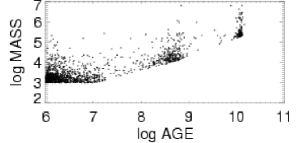
Figure 2.: 2a (upper left) - Continuous formation model; 2b (upper right) continuous formation model convolved with a magnitude threshold; 2c (lower left) - observed data from the Antennae (Fall, Chandar, Whitmore 2004); 2d (lower right) early version of toy model for the Antennae with continuous formation for the last 10¹⁰ years, an additional continuous formation “burst” for the last 100 Myr, Gaussian bursts at 500 Myr and 12 Gyr, and infant mortality plus constant mass loss destruction laws. Artifacts include the 10³ M_⊙ cutoff artifact for the simulations, and the apparent gap around 10 Myr in the Antennae observations (due to age-dating difficulties).

If one looks closely at Figure 3 there actually are small differences on different chips (e.g., the “overlap” region portion of WF3 has the largest number of very young clusters), but these are secondary effects; the primary correlation is the rapid decline in the number of clusters as a function of age.

3.3. Insight 3 - Early Results from the Inclusion of Destruction Laws

Three heuristic destruction laws have been incorporated into the toy model at present: 1) constant mass loss (e.g., typical values of 10^-5 M_⊙/yr result in reasonable looking models), 2) the Lamers model (e.g., Boutloukous & Lamers, 2003), and 3) infant mortality (parameterized in this simple model as random removal of 90 % of the clusters every decade of log(time) for the first 100 Myrs).

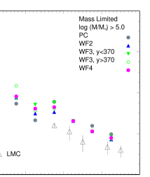
Figure 3.: The log(dn/dt) vs. log(time) diagram for the Antennae with results for the four WFPC2 chips shown separately (normalized at log(age) = 8.2). The WF3 chip is broken into two regions; one being the very active “overlap” region (y $>$ 370), the other being a region outside the overlap region in an area with a high proportion of older clusters (y $<$ 370). The open triangles show the trends in the LMC (Elson & Fall 1985).

We note that the Lamers model with values of T4=100 Myr (appropriate for their results on M33 and M51) predicts that even a cluster with 10⁶ M_⊙ is destroyed in $\approx$ 1 Gyr, implying that no young clusters evolve to become old globular clusters ! We also note that the Lamers formula predicts essentially no destruction occurs until about 100 Myr, implying that all young clusters are bound and that the infant mortality rate is zero. These are likely to be artifacts of an empirically determined model fit over a limited age range. Care must be used to only use this model in the appropriate age range.

4. The Antennae as a Scaled-Up Version of the Milky Way

Lada & Lada (2003) make several of the same points about the need for infant mortality for the Milky Way that are made for the Antennae in this paper, even to the level of giving the same numbers (i.e., 90 % destruction after 10 Myr)! In fact, it is possible to view the Antennae as a scaled-up version of the Milky Way. According to Lada & Lada (2003), the Milky Way has roughly 100 known embedded young clusters within a radius of $\approx$ 2 kpc. The most massive clusters in this sample are slightly larger than 10³ M_⊙. If we were able to see the entire disk of the Milky Way the sample would be roughly 100 times larger. The star formation rate per unit area in the Antennae is also roughly a factor of 10 higher than the Milky Way (Zhang, Fall, & Whitmore 2003) hence the total enhancement for the number in the sample might be roughly a factor of 1000. Assuming a universal power law with index –2 for the initial mass function, the most massive clusters with comparable ages to the Lada & Lada sample (i.e., $\approx$ 10 Myr) would be predicted to be $\approx$ 10⁶ M_⊙, just as they are in the Antennae.

5. An Objective Classification System for Star Clusters

Several authors (e.g., Whitmore 2003, Terlevich 2004) have pointed out the large number of different names used to describe basically similar objects (i.e., super star clusters, young massive clusters, populous clusters, young globular clusters, …). Conversely, other authors (e.g., Hodge 1988, see Figure 2 for a dramatic example) have pointed out how dissimilar objects that we call globular can be.

It may be beneficial to consider an objective classification system that would help unify the situation. Such a system would also provide a more meaningful method of comparing clusters in different galaxies, near and far.

Hodge (1988) suggested an objective 3-dimensional classification system for star clusters consisting of mass, age, and metallicity. While the first two parameters are clearly fundamental, metallicity appears to be less important in a dynamical sense and is largely correlated with age in any case. In the context of our statement that understanding the destruction of clusters will be critical to understanding their demographics, a better choice for the third parameter might be the density or size of a cluster, which largely controls how susceptible a cluster is to destruction. As pointed out by Terlevich (private communication), size would be the better choice since density is a derived quantity.

References

- (1) Barmby, P. 2002, IAUS, 207, 58
- (2) Billett, O. H., Hunter, D. A. & Elmegreen, B. G. 2002, AJ, 123, 1454
- (3) Boutloukous, S. G. & Lamers, H. J. G. L. M. 2003, MNRAS, 338, 717
- (4) Chandar, R. & Whitmore, B. C. 2004, in preparation
- (5) Chandar, R. & Bianchi, L., Ford, H. C., & Salasnich, B. 1999, PASP, 111, 794
- (6) de Grijs, R., Anders, P., Bastian, N., Lynds, R., Lamers, H. J. G. L. M., O’Neil, E. J. 2003, MNRAS, 343, 161.
- (7) Elmegreen, B. G. & Efremov, Y. N. 1997, ApJ, 480, 235
- (8) Elson, R. A. W. & Fall, S. M. 1985, ApJ, 299, 211
- (9) Fall, S. M. & Rees, M. J. 1977, MNRAS, 181, 37P
- (10) Fall, S. M. & Zhang, Q. 2001, ApJ, 561, 751
- (11) Fall, S. M. 2004, this volume.
- (12) Fall, S. M., Chandar, R. & Whitmore, B. C. 2004, in preparation.
- (13) Gnedin, O. & Ostriker, J. P. 1997, ApJ, 474, 223
- (14) Harris, J., Calzetti, D., Gallagher, J. S., Conselice, C. J., Smith, Denise A. 2001, AJ, 122, 3046
- (15) Hodge, P. 1988, PASP, 100, 568
- (16) Hunter, D. A., Elmegreen, B. G., Dupuy, T. J., Mortonson, M. 2003, AJ, 126, 1836
- (17) Lada, C. J. & Lada, E. A. 2003, ARAA, 41, 57
- (18) Larsen, S. S. 2002, AJ, 124, 1393
- (19) Larsen, S. S. & Richtler, T. 2000, A&A, 354, 836
- (20) Terlevich, R. 2004, this volume
- (21) Vesperini, E. 1998, MNRAS, 299, 1019
- (22) Whitmore, B. C. 2003, in A Decade of HST Science, eds. Mario Livio, Keith Noll & Massimo Stiavelli, (Cambridge: Cambridge University Press), 153. (widely referenced as Whitmore 2000, astro-ph/0012546)
- (23) Whitmore, B. C., Zhang, Q., Leitherer, C., Fall, S. M., Schweizer, F. & & Miller, B. W. 1999, AJ, 118, 1551
- (24) Zhang, Q., Fall, M. & Whitmore, B. C. 2001, ApJ, 561, 727
- (25) Zhang, Q. & Fall 1999, ApJ 527, L81