Measurements of Primary and Atmospheric Cosmic-Ray Spectra with the BESS-TeV Spectrometer

Abstract

Primary and atmospheric cosmic-ray spectra were precisely measured with the BESS-TeV spectrometer. The spectrometer was upgraded from BESS-98 to achieve seven times higher resolution in momentum measurement. We report absolute fluxes of primary protons and helium nuclei in the energy ranges, 1–540 GeV and 1–250 GeV/n, respectively, and absolute flux of atmospheric muons in the momentum range 0.6–400 GeV/$c$.

, , , , , , , , , , , , , , , , , , , , , , , , , , , , , , , ,

1 Introduction

The absolute flux and spectral shape of primary cosmic rays are the basis to discuss the origin and the propagation history of the cosmic rays in the Galaxy. The spectrum is also essential as an input to calculate spectra of cosmic-ray antiprotons and positrons which are secondary products of cosmic-ray interactions with the interstellar gas. Recently, the importance of the cosmic-ray spectrum has been emphasized in connection with the study of neutrino oscillation observed in atmospheric neutrinos [2]. In contrast with a long-baseline experiment, such as K2K [3], the feature of the oscillation study with atmospheric neutrinos lies in its wide energy range. For example, the Super Kamiokande water Cherenkov detector [4] can observe neutrinos from 0.1 to 100 GeV. In order to estimate an accurate flux of atmospheric neutrinos up to around 100 GeV, we need to know the primary cosmic-ray flux well above 100 GeV and the feature of hadronic interactions in that energy region. It is crucial to measure primary cosmic-ray flux by determining the absolute energy of particles. Measurements of atmospheric muon spectrum is also important to check and improve our understanding of hadronic interactions.

The Balloon-borne Experiment with a Superconducting Spectrometer (BESS) [5, 6] has been carried out since 1993 to perform highly sensitive searches for cosmic-ray antiparticles and precise measurements of absolute flux of various cosmic-ray components. The absolute fluxes of primary protons and helium nuclei were precisely measured in the energy ranges, 1–120 GeV and 1–54 GeV/n, respectively, by a balloon observation in 1998 [7]. The overall uncertainties in the measurements were less than 5 % for protons and 10 % for helium nuclei. The absolute flux of atmospheric muons was measured from 0.6 to 20 GeV/$c$ at sea level [8] and from 0.6 to 100 GeV/$c$ at a mountain altitude [9]. The overall uncertainty in the measurements was less than 10 %. In order to extend the energy range of the precise measurements of cosmic-ray flux up to higher energy, the BESS-TeV spectrometer was developed. A magnetic rigidity ($R\equiv pc/Ze$) of an incident particle was accurately measured by a new tracking system. The maximum detectable rigidity (MDR) was significantly improved from 200 GV to 1.4 TV.

Cosmic-ray observations were carried out with the BESS-TeV spectrometer at a balloon altitude and at sea level in 2002. We report precise measurements of absolute fluxes of primary protons and helium nuclei, and atmospheric muons.

As to primary cosmic rays, we focused on a energy range above 1 GeV/n in this paper. The BESS spectrometer has measured primary cosmic-ray flux down to 0.2 GeV/n, which provides significant information on the solar modulation effect and the propagation of cosmic rays [10]. Measurements of the low-energy cosmic-ray flux with the BESS-TeV spectrometer will be reported elsewhere together with a series of BESS balloon-flight data [11].

2 The BESS-TeV spectrometer

The BESS spectrometer [12] was upgraded to achieve a significantly high rigidity resolution. The upgraded spectrometer, “BESS-TeV” [13], was equipped with newly-developed drift chambers.

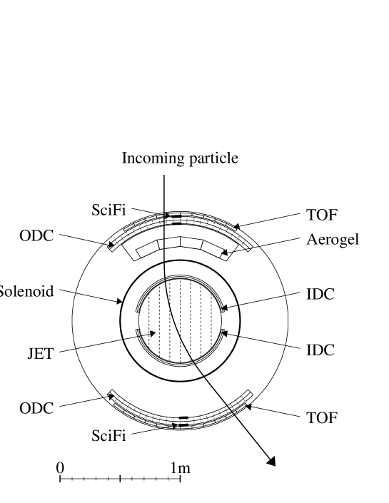
Figure 1: Cross-sectional view of the BESS-TeV spectrometer.

As shown in Fig. 1, the detector has a unique feature of a cylindrical configuration realized by a thin superconducting solenoid [14]. The configuration resulted in a large and almost constant geometrical acceptance and a uniform detector performance for various incident angles and positions.

In the central region, the solenoid with a diameter of 1 m provides a uniform magnetic field of 1 T. The field variation is less than 2.5 % along a typical trajectory of an incoming particle. A deflection ($R^{-1}$) of the trajectory is measured by a central jet-type drift chamber (JET), two inner drift chambers (IDCs) and two outer drift chambers (ODCs), all of which were newly developed for the BESS-TeV spectrometer. Inside JET and IDCs a trajectory was determined by simple circular fitting [15] using up to 52 hit points. Each hit point was measured with a spacial resolution of 150 $\mu$m. More accurate deflection was measured by adding 8 hit points inside ODCs which are placed outside the solenoid at a radius of 0.8 m. The hit positions inside the ODCs were used above 100 GV, where the effect of multiple scattering in the detector material is negligibly small. Fig. 2 shows a distribution of the deflection resolution ($\Delta R^{-1}$) obtained with all the drift chambers. The deflection resolution was evaluated in the track-fitting procedure for cosmic-ray protons. Those of other spectrometers used in previous balloon experiments [7, 16, 17] are also shown. Each area of the histogram is normalized to unity. The peak position of 0.7 TV^-1 corresponds to the MDR of 1.4 TV. In order to provide an absolute reference position for their calibration, a scintillating fiber counter system (SciFi) was attached to the top and the bottom walls of the ODCs. SciFi consists of two layers of 1 mm $\times$ 1 mm square-shaped scintillating fibers and covers the central cell of each ODC. The scintillating fiber layers are shifted by 0.5 mm with each other. SciFi can measure a hit position with an accuracy of the overlap width of two fiber layers, i.e. 0.5 mm. With a sufficiently large number of events, the track position can be determined with a better spatial resolution than that of ODCs.

Time-of-flight (TOF) hodoscopes [18] provide the velocity ($\beta$) and energy loss (d$E$/d$x$) measurements. A $\beta^{-1}$ resolution of 1.4 % was achieved in the experiment. The data acquisition sequence is initiated by a first-level TOF trigger, which is a simple coincidence of signals from the upper and lower TOF counters. The trigger efficiency was evaluated to be 99.4$\pm$0.2 % by a secondary proton beam at KEK 12 GeV proton synchrotron. The trigger rates were 1 kHz and 30 Hz at a balloon altitude and sea level, respectively. During the balloon observation, one out of every ten events were recorded to sample unbiased trigger events. An auxiliary trigger is generated by a signal from a Cherenkov counter [19] to record particles above threshold energy without bias or sampling. The efficiency of the Cherenkov trigger was evaluated as the ratio of the number of Cherenkov-triggered events to the unbiased triggered events. It was found to be 94.1$\pm$ 2.0% and 97.3$\pm$4.0 % for relativistic protons and helium nuclei, respectively. For the determination of primary proton and helium fluxes, the Cherenkov-triggered events were used above 10 GeV and 5.5 GeV/n, respectively, and the TOF-triggered events were used below these energies. During the ground observation, all the TOF-triggered events were recorded to determine the atmospheric muon flux.

3 Observations

The BESS-TeV spectrometer was launched by a balloon from Lynn Lake, Manitoba, Canada (56.5^∘N, 101.0^∘W), on 7th August 2002. After about four-hour ascending, the payload reached a floating altitude of 37 km (residual atmosphere of 4.8 g/cm²). The geomagnetic cutoff rigidity was 0.5 GV or smaller throughout the flight. The total live time of the data-taking was 38,215 seconds (10.6 hours) during the floating period. Among them 11 % (1.2 hours) of data taken around the sun rise were not used in this analysis, because the rapid temperature variation might introduce a large systematic error in the chamber calibration.

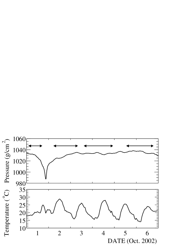
Figure 3: Atmospheric pressure and temperature during the ground observation. Arrows indicate the data-taking periods used to determine the atmospheric muon flux. The atmospheric temperature data were obtained from Ref. [20].

The ground observation was carried out at KEK located at Tsukuba, Japan (36.2^∘N, 140.1^∘W), during a period of 1st–6th October 2002. Tsukuba is located 30 m above sea level with the vertical cutoff rigidity of 11.4 GV. The variations in the atmospheric pressure and temperature during the observation are shown in Fig. 3. The atmospheric temperature data were obtained from Ref. [20]. The arrows indicate the data-taking periods used to determine the atmospheric muon flux. We did not use the data during a period where the variation in atmospheric pressure was large. The mean (root-mean-square) atmospheric pressure and temperature during the periods used for the flux determination were 1032.2 g/cm² (4.4 g/cm²) and 20.8 ^∘C (3.7 ^∘C), respectively. The total live time of the data-taking was 329,403 seconds (91.5 hours).

4 Data analysis

4.1 Event reconstruction

Each hit position inside the drift chambers was calculated from the drift time digitized by a flash analog-to-digital converter. The calculation was carried out based on a relation between the hit position and the drift time ($x$-$t$ relation). The $x$-$t$ relation was precisely calculated by a drift chamber simulation package, GARFIELD [21], and a gas property simulation package, MAGBOLTZ [22]. Although the chambers were constructed carefully with a tolerance of 100 $\mu$m, there was a small position deviation of wires and field-shaping patterns, which could locally modify the electric field. In order to take account of the limited accuracy in the chamber manufacturing, a correction was commonly applied to the calculated $x$-$t$ relation throughout the experiments. The correction was obtained to minimize the $\chi^{2}$ in the fitting of straight tracks of clean muon events observed on the ground without magnetic field. The correction was as small as expected from the accuracy in the chamber manufacturing. During the observations, the $x$-$t$ relation was affected by the variation in the pressure and temperature of the chamber gas. In order to take account of these time-dependent variations, the $x$-$t$ relation was calibrated for each data-taking run. Especially in calibrating the $x$-$t$ relation of ODCs, an absolute reference positions were provided by SciFi, which are not affected by the variation in the pressure nor temperature.

The same calibration procedure was applied to the muon events observed on the ground without magnetic field, where the straight tracks were used as an absolute reference of events with infinite rigidity. We checked the deflection of the muon events by applying circular-fitting to the calibrated hit points inside the JET and IDCs. The mean value of the obtained deflection was smaller than (10 TV)^-1. Therefore, the systematic shift in the deflection measurement originated from this calibration procedure should be smaller than (10 TV)^-1.

The precise alignment of the ODCs with respect to the JET was determined by checking the consistency between tracks reconstructed by JET and hit points measured by ODCs. In order to minimize the effect of multiple scattering in the detector material, we selected events whose rigidity was measured to be higher than 4 GV by JET and IDCs. The chamber alignment was calibrated for each run. We checked the variation in the calibrated position of ODCs in 84 runs during the ground observation. The root-mean-square of the variation was smaller than 20 $\mu$m. This variation might introduce a systematic error in the deflection measurement of $\Delta R^{-1}$ = (5.3 TV)^-1.

4.2 Event selection

We selected events with a single track fully contained inside the fiducial volume defined by the central six columns out of eight columns in the JET. It ensured that the track is long enough for reliable rigidity measurement. In order to obtain a nearly vertical flux of atmospheric muons, an additional cut on the zenith angle ($\theta_{\rm z}$) was applied as $\cos\theta_{\rm z}>0.98$ below 20 GV and $\cos\theta_{\rm z}>0.90$ above 20 GV. We have checked the change of the atmospheric muon flux above 20 GV by requiring two conditions, $\cos\theta_{\rm z}>0.98$ and $\cos\theta_{\rm z}>0.90$. We found that the requirement to zenith angle could be relaxed to $\cos\theta_{\rm z}>0.90$ without changing the observed flux. For protons and helium nuclei zenith angle cut was not applied. Due to the detector geometry, however, zenith angle is limited as $\cos\theta_{\rm z}>0.80$ above 2 GV.

A single-track event was defined as an event which has only one isolated track inside the JET and one or two hit counters in each layer of the TOF hodoscopes. The single-track selection eliminated rare interacting events. To estimate the efficiency of the single-track selection, Monte Carlo simulations with GEANT3/4 [23, 24] were performed. The probability that each particle could pass through the selection was evaluated by applying the same selection criteria to the Monte Carlo events. The resultant efficiency of the single-track event selection for protons was 82.0$\pm$2.6 % at 20 GV and 79.9$\pm$4.0 % at 200 GV, the efficiency for helium nuclei was 69.6$\pm$6.6 % at 20 GV and 66.9$\pm$7.2 % at 200 GV, and the efficiency for muons was 96.8$\pm$1.5 % at 20 GV and 95.9$\pm$1.5 % at 200 GV. In order to ensure the track reconstruction in the $z$-direction (perpendicular to the bending plane), we required a consistency of hit position in the $z$-direction measured by two independent detectors; the drift chamber and the TOF hodoscope. The efficiency of this selection was estimated to be 97.2$\pm$1.0 % for protons, 95.5$\pm$1.5 % for helium nuclei, and 98.1$\pm$1.0 % for muons.

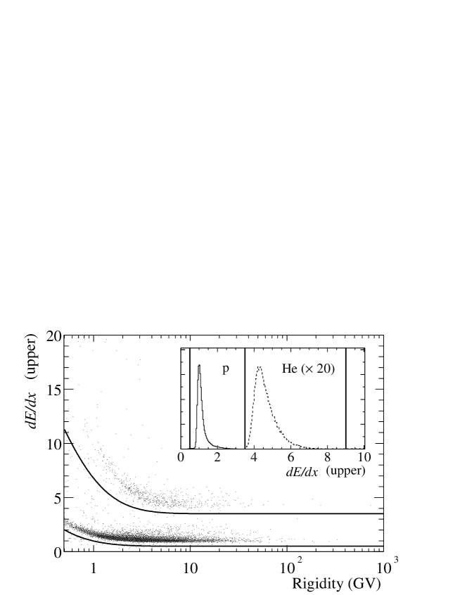
Figure 4: Proton band in d$E$/d$x$ (top TOF) vs. rigidity obtained from the balloon observation. A d$E$/d$x$ in the bottom TOF was also checked. The superimposed graph shows the selection criteria for protons and helium nuclei above 10 GV.

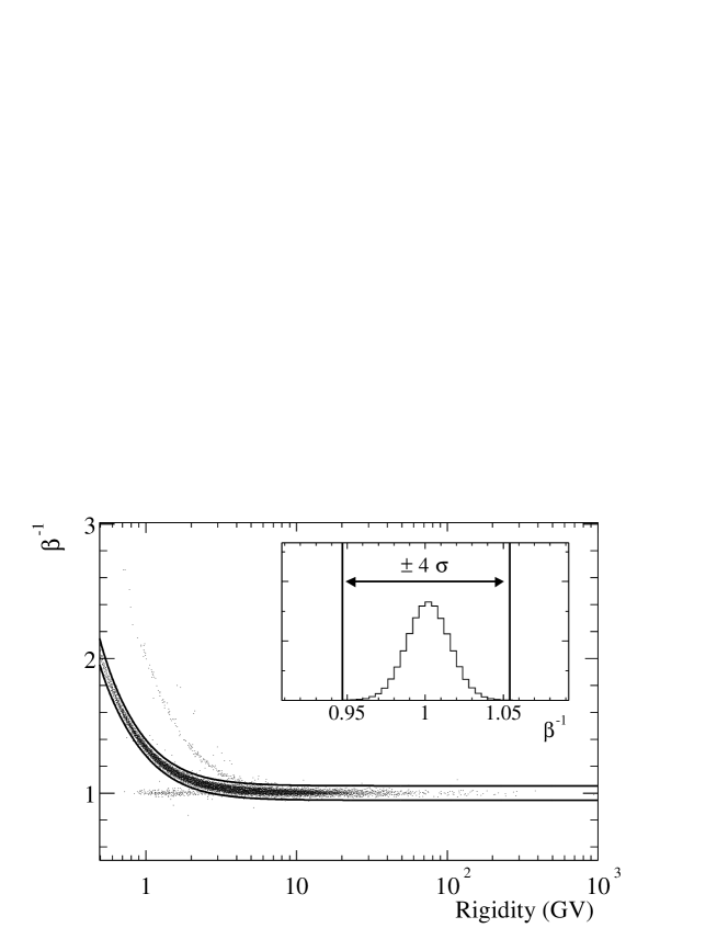
Figure 5: Scatter plot of $\beta^{-1}$ vs. rigidity obtained from the balloon observation after proton d$E$/d$x$ selection. The superimposed graph shows the selection criteria for protons above 10 GV.

Particle identification was performed by requiring proper d$E$/d$x$ measurements with both upper and lower layers of the TOF hodoscopes and $\beta^{-1}$ as functions of rigidity. Figs. 4 and 5 show the selection criteria for protons. Helium nuclei and muons were identified in the same manner. The efficiencies of d$E$/d$x$ selection were estimated with another sample selected by independent measurement of energy loss inside the JET. We found that 96.3$\pm$0.3 % of protons, 92.3$\pm$0.9 % of helium nuclei and 99.9$\pm$0.1 % of muons were properly identified. Since the $\beta^{-1}$ distribution is well described by Gaussian and a half-width of the $\beta^{-1}$ selection band was set at 4 $\sigma$, the efficiency is very close to unity. Following this particle identification procedure, 444,578 proton, 38,006 helium, and 688,983 muon candidates were obtained.

4.3 Backgrounds

As shown in Fig. 5, protons were identified without contamination by examining $\beta^{-1}$ distribution below 2 GV. Above 2 GV, there were contamination of light particles such as positrons, pions and muons. The ratio of light particles to protons was observed to be 4.5 % at 1 GV and 1.1 % at 2 GV, which was expressed by a power law with an index of $-2.1$. This tendency was reproduced well by a Monte Carlo simulation [25] based on the DPMJET-III event generator [26]. Above 10 GV, the simulated $\mu^{+}$/p ratio shows almost constant value of 0.2 %. In this analysis the contamination of the light particles were subtracted by assuming the power law, which would underestimate the background of light particles. However, The contamination is smaller than the statistical errors. Above 3 GV, there were contamination of deuterons, which was observed to be 2 % at 3 GV. According to our previous measurement [10], the d/p flux ratio decreases with increasing rigidity. The ratio should follow a decrease in escape path lengths of primary cosmic-ray nuclei [27]. Since the contamination of deuterons was as small as the statistical errors, and should decrease with increasing rigidity, no subtraction was made for the deuteron contamination. Therefore, above 3 GV hydrogen nuclei were selected, which included a small amount of deuterons. Helium nuclei were identified clearly by redundant charge measurement inside the upper and lower TOF hodoscopes. The helium candidates contained both ³He and ⁴He. In conformity with previous experiments, all doubly charged particles were treated as ⁴He.

Among the muon candidates observed on the ground, there were contaminations of electrons, positrons and protons. In our previous work, the ratio of electrons and positrons to muons was measured to be 1.5 % at 0.5 GV and 0.3 % at 1 GV with an electro-magnetic shower counter [8]. Since the BESS-TeV spectrometer is not equipped with an electro-magnetic shower counter, no subtraction was made for the contamination of electrons and positrons. However, the contamination was smaller than the statistical errors. Protons were identified by examining $\beta^{-1}$ distribution below 2.5 GV. The p/$\mu$ flux ratio was observed to be 3.3 % at 1 GV and 1.2 % at 2.5 GV, which was expressed by a power law with an index of $-1.0$. Below 7 GV, the power law agreed well with a previous measurement of the p/$\mu$ ratio [28], which shows, however, constant value of about 0.4 % above 7 GV. The proton background was subtracted from muon candidates assuming the power law below 7 GV and constant value of 0.4 % above 7 GV.

4.4 Normalization and corrections

In order to obtain the absolute flux of protons, helium nuclei and muons at the top of the detector, energy loss by ionization inside the detector material, live time and geometrical acceptance were estimated. The energy of each incoming particle was calculated by integrating the energy losses inside the detector tracing back along the particle trajectory. The total live time of the data-taking was measured exactly by counting 1 MHz clock pulses with a scaler system gated by a “ready” status that controls the first-level trigger. The geometrical acceptance defined for this analysis was calculated as a function of rigidity with a simulation technique [29]. The geometrical acceptance is 0.0886$\pm$0.0003 m²sr for protons and helium nuclei at 10 GV and 0.0302$\pm$0.0001 m²sr for muons at 10 GV. The acceptance for muons is about 1/3 of that for protons and helium nuclei because of the additional requirement on the zenith angle ($\cos\theta_{\rm z}>0.98$) as described in Section 4.2. The simple cylindrical shape and the uniform magnetic field make it simple and reliable to determine the geometrical acceptance precisely. The error on the acceptance calculation was estimated to be 0.3 % which represents the uncertainty of the detector alignment

In order to obtain the absolute flux of primary protons and helium nuclei at the top of the atmosphere, interaction loss and secondary particle production in the residual atmosphere were estimated. According to the Monte Carlo studies, probabilities for primary cosmic rays to penetrate the residual atmosphere of 4.8 g/cm² are 93.8$\pm$0.7 % and 91.3$\pm$2.0 % for protons and helium nuclei, respectively, at 10 GeV and almost constant over the entire rigidity range discussed here. Atmospheric secondary protons were subtracted based on a calculation for the maximum solar activity epoch by Papini et al. [30]. A secondary-to-primary proton ratio is 4.8$\pm$0.5 % at 1 GeV and 1.7$\pm$0.2 % above 10 GeV. Atmospheric secondary helium nuclei above 1 GeV/n are dominated by the fragments of heavier cosmic-ray nuclei (mainly carbon and oxygen). The flux ratio of the atmospheric secondary helium to the primary carbon and oxygen was estimated to be 14 % at a depth of 4.8 g/cm², based on the total inelastic cross sections of CNO+Air interactions and the helium multiplicity in ¹²C + CNO interactions [31]. The total correction of atmospheric secondary helium produced by all the primary nuclei with Z$>$2 was estimated to be 1.6$\pm$0.5 % at 1 GeV/n and 2.1$\pm$0.6 % at 10 GeV/n.

4.5 Spectrum deformation effect

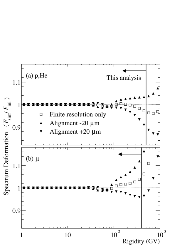
Figure 6: Spectrum deformation effects for (a) primary protons and helium nuclei and (b) atmospheric muons. The deformation effects are shown as ratios of simulated spectra ($F_{\rm sim}$) to the input spectra ($F_{\rm ini}$) as functions of rigidity. Open squares show the case when ODCs are aligned correctly. Upward and downward triangles show the case when ODCs are artificially displaced by $\pm 20\mu$m.

Because of the limited accuracy of the rigidity measurement and the steep spectral shape, the observed spectrum may suffer deformation. The limited accuracy of the rigidity measurement was decomposed into two sources: (i) a finite resolution in the rigidity measurement, and (ii) a small shift in the measured deflection which is caused by the misalignment of the ODCs. We estimated the systematic error in the spectrum measurement caused by such limited accuracy of the rigidity measurement. The systematic error was estimated by a Monte Carlo simulation. In the simulation, detailed response of the drift chamber was implemented, such as the distribution of primary ionization clusters, the diffusion in the gas, the fluctuation of avalanche gain, and the digitization in the readout electronics. The simulated rigidity resolution reproduced well the experimental result shown in Fig. 2. Therefore the effect of spectrum deformation should be correctly estimated by this simulation. As an input spectrum, a power-law function was used with a spectral index of $-2.7$ for both primary protons and helium nuclei. For atmospheric muons, the spectral index was chosen as $-3.2$, which was obtained by fitting a power-law function to the muon spectrum obtained with this experiment in the rigidity range 100–400 GV. Fig. 6 shows the effect of spectrum deformation as a ratio of simulated spectrum to the input spectrum. The open squares show the spectrum deformation when ODCs are aligned correctly. In this case, the deformation is caused only by the effect of (i). The change of the spectrum is less than 5 % for protons and helium nuclei below 1 TV, and for muons below 400 GV. The upward and downward triangles show the spectrum deformation when ODCs are artificially displaced by $\pm 20\mu$m. We found that the shift of the measured deflection was smaller than (5.3 TV)^-1 as described in Section 4.1. The change of the spectrum was less than 2 % below 100 GV and 10 % at 500 GV for primary protons and helium nuclei, and less than 3 % below 100 GV and 13 % at 400 GV for muons. Since the input spectrum of atmospheric muons is steeper than that of primary protons and helium nuclei, the spectrum deformation effect is more significant for atmospheric muons. We did not apply any corrections, such as unfolding, on the observed spectra. The spectrum deformation effect estimated above was treated as a systematic error on the observed spectra, which was as small as the statistical error over the entire rigidity range in this analysis.

5 Results and discussions

We have obtained the absolute fluxes of primary protons in the range 1–540 GeV and helium nuclei in the range 1–250 GeV/n at the top of the atmosphere from the BESS-TeV balloon-flight data in 2002. We have obtained the absolute flux of muons in the range 0.6–400 GeV/$c$ at sea level (30 m a.s.l.) from the BESS-TeV ground-observation data in 2002. The results of protons and helium nuclei are summarized in Tables 1 and 2, respectively, and the results of atmospheric muons are summarized in Table 3. The overall uncertainties including both statistical and systematic errors were less than $\pm$15 % for protons, $\pm$20 % for helium nuclei, and $\pm$20 % for muons.

The results of primary proton and helium spectra are shown in Fig. 7 in comparison with other experiments with magnetic spectrometers [7, 16, 17, 32, 33, 34]. Discrepancies in the observed spectra below 10 GeV for protons and 5 GeV/n for helium nuclei come from the difference of solar activity (around minimum in 1998 and around maximum in 2002). The detailed analysis of the solar modulation affecting the low-energy spectra in a series of BESS flights will be discussed elsewhere [11].

Although a small systematic shift of 2–3 % was found in absolute proton flux between the results of BESS-TeV and BESS-98 from 30 to 100 GeV, the results are well consistent within the overall uncertainty of 5 %. The main source of this uncertainty was the aerogel trigger efficiency. The accuracy of the efficiency estimation was limited by the statistics of the event sample to be 2.0 % and 3.0 % for BESS-TeV and BESS-98, respectively.

Our resultant spectral shape of protons and helium nuclei is very similar to that measured by AMS [32, 33]. Above 30 GeV, the absolute proton flux measured by BESS-TeV and AMS shows good agreement within 5 %. However, there is 15 % discrepancy in the absolute flux of helium nuclei. Both proton and helium spectra by CAPRICE-98 [16] show steeper spectra than our results.

At high energies, the spectrum $F$ may be parameterized by a power law in kinetic energy, $E_{\rm k}$, as $F=\Phi E_{\rm k}^{-\gamma}$. The fitting range was chosen to be 30–540 GeV for protons and 20–250 GeV/n for helium nuclei so that the solar modulation effect was negligible. The best fit values and uncertainties for protons ($\Phi_{\rm p}$ and $\gamma_{\rm p}$) and helium nuclei ($\Phi_{\rm He}$ and $\gamma_{\rm He}$) were obtained as

$$\Phi_{\rm p}=(1.37\pm 0.06({\rm sta.})\pm 0.11({\rm sys.}))\times 10^{4}~{}(\rm m^{2}\cdot sr\cdot s\cdot GeV)^{-1}$$

$$\gamma_{\rm p}=2.732\pm 0.011({\rm sta.})\pm 0.019({\rm sys.})$$

and

$$\Phi_{\rm He}=(7.06\pm 0.94({\rm sta.})\pm 1.17({\rm sys.}))\times 10^{3}~{}(\rm m^{2}\cdot sr\cdot s\cdot(GeV/n))^{-1}$$

$$\gamma_{\rm He}=2.699\pm 0.040({\rm sta.})\pm 0.044({\rm sys.})$$

respectively. The two parameters were strongly correlated, with a correlation coefficient of $-0.98$.

The result of atmospheric muon spectrum is shown in Fig. 8 in comparison with other absolute flux measurements by magnetic spectrometers [8, 9, 35, 36]. The discrepancy below 30 GeV/$c$ among the observed muon spectra is mainly due to the difference in altitudes. Fig. 9 shows charge ratios of atmospheric muons observed in a series of muon measurement with the BESS experiments. The difference in the charge ratios observed in Japan and Canada comes from the different geomagnetic cutoff rigidity [8].

6 Conclusion

We have measured energy spectra of primary protons in the range 1–540 GeV and helium nuclei in the range 1–250 GeV/n by a balloon observation, and momentum spectrum of atmospheric muons in the range 0.6–400 GeV/$c$ by a ground observation at sea level.

The overall uncertainties were less than 15 % for protons, less than 20 % for helium nuclei, and less then 20 % for muons. Primary cosmic-ray spectra provide fundamental information on the origin and propagation history of the cosmic rays. The results also provide accurate input spectra to predict an atmospheric neutrino flux. The result of atmospheric muon spectrum will improve the accuracy of atmospheric neutrino calculation in the wide momentum range.

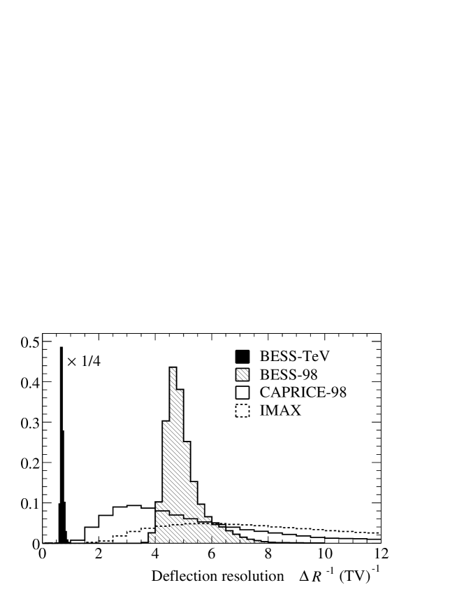
Figure 2: Distribution of the deflection resolution for protons evaluated for each event in the track-fitting procedure. Each area of the histogram is normalized to unity.

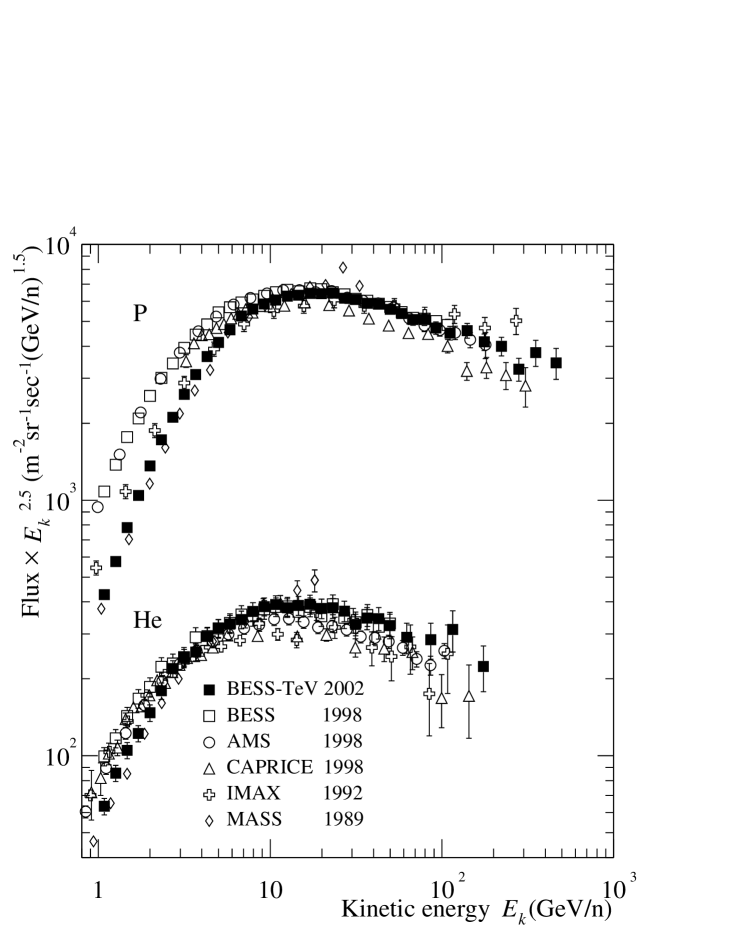
Figure 7: Absolute differential energy spectra of primary protons and helium nuclei multiplied by $E_{k}^{2.5}$. The spectra obtained by other experiments [7, 16, 17, 32, 33, 34] are also shown.

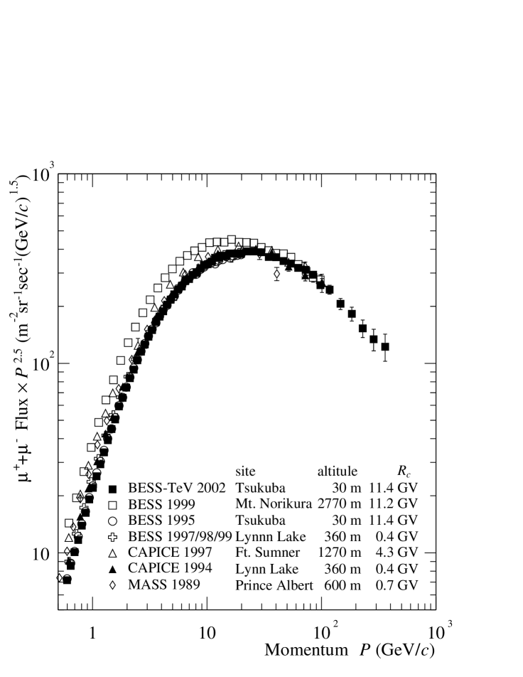
Figure 8: Absolute differential momentum spectrum of atmospheric muons multiplied by $P^{2.5}$. The spectra obtained by other experiments [8, 9, 35, 36] are also shown. The geomagnetic cutoff rigidity at each site is indicated as $R_{c}$. The difference below 30 GeV/$c$ among the spectra is mainly due to the different altitudes.

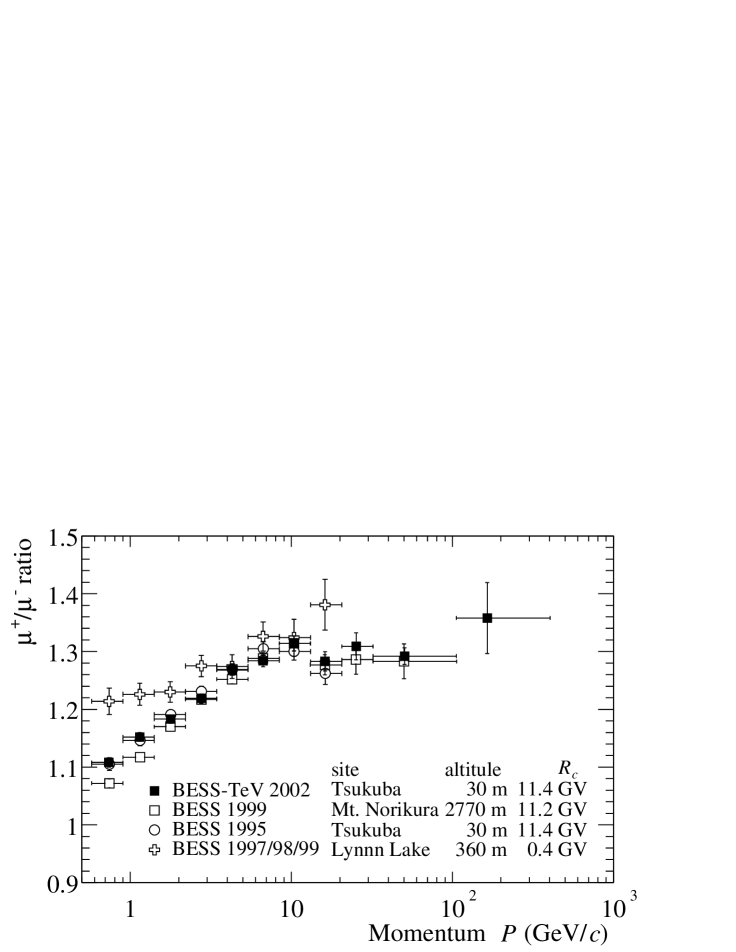
Figure 9: Charge ratios of atmospheric muons. Only statistical errors are included. The charge ratios obtained by other experiments [8, 9] are also shown. The geomagnetic cutoff rigidity at each site is indicated as $R_{c}$. The difference among the charge ratios is mainly due to the difference in geomagnetic cutoff rigidity.

Table 1: Primary proton flux at the top of the atmosphere.

Energy range (GeV)		$\overline{E_{\rm k}}$ (GeV)	Flux$\pm\Delta F_{\rm sta}\pm\Delta F_{\rm sys}$ (m-2sr-1s-1GeV-1)
1.00–	1.17	1.08	3.50 $\pm$0.03 $\pm$0.11 $\times 10^{2}$
1.17–	1.36	1.26	3.22 $\pm$0.03 $\pm$0.10 $\times 10^{2}$
1.36–	1.58	1.47	2.98 $\pm$0.02 $\pm$0.09 $\times 10^{2}$
1.58–	1.85	1.71	2.71 $\pm$0.02 $\pm$0.08 $\times 10^{2}$
1.85–	2.15	2.00	2.41 $\pm$0.02 $\pm$0.07 $\times 10^{2}$
2.15–	2.51	2.33	2.08 $\pm$0.02 $\pm$0.06 $\times 10^{2}$
2.51–	2.93	2.71	1.74 $\pm$0.01 $\pm$0.05 $\times 10^{2}$
2.93–	3.42	3.16	1.45 $\pm$0.01 $\pm$0.04 $\times 10^{2}$
3.42–	3.98	3.69	1.19 $\pm$0.01 $\pm$0.03 $\times 10^{2}$
3.98–	4.64	4.30	9.52 $\pm$0.08 $\pm$0.27 $\times 10^{1}$
4.64–	5.41	5.01	7.35 $\pm$0.07 $\pm$0.21 $\times 10^{1}$
5.41–	6.31	5.84	5.63 $\pm$0.05 $\pm$0.16 $\times 10^{1}$
6.31–	7.36	6.81	4.34 $\pm$0.04 $\pm$0.12 $\times 10^{1}$
7.36–	8.58	7.93	3.15 $\pm$0.03 $\pm$0.09 $\times 10^{1}$
8.58–	10.0	9.25	2.25 $\pm$0.03 $\pm$0.06 $\times 10^{1}$
10.0–	11.7	10.8	1.59 $\pm$0.01 $\pm$0.05 $\times 10^{1}$
11.7–	13.6	12.6	1.12 $\pm$0.01 $\pm$0.04 $\times 10^{1}$
13.6–	15.8	14.7	7.71 $\pm$0.04 $\pm$0.28
15.8–	18.5	17.1	5.33 $\pm$0.03 $\pm$0.20
18.5–	21.5	19.9	3.63 $\pm$0.02 $\pm$0.14
21.5–	25.1	23.2	2.48 $\pm$0.02 $\pm$0.10
25.1–	29.3	27.1	1.62 $\pm$0.01 $\pm$0.06
29.3–	34.1	31.6	1.09 $\pm$0.01 $\pm$0.04
34.1–	39.8	36.8	7.17 $\pm$0.08 $\pm$0.30 $\times 10^{-1}$
39.8–	46.4	42.9	4.84 $\pm$0.06 $\pm$0.21 $\times 10^{-1}$
46.4–	54.1	50.0	3.15 $\pm$0.05 $\pm$0.14 $\times 10^{-1}$
54.1–	63.1	58.3	2.07 $\pm$0.03 $\pm$0.09 $\times 10^{-1}$
63.1–	73.6	68.0	1.34 $\pm$0.03 $\pm$0.06 $\times 10^{-1}$
73.6–	85.8	79.2	9.09 $\pm$0.19 $\pm$0.43 $\times 10^{-2}$
85.8–	100.	92.3	5.75 $\pm$0.14 $\pm$0.28 $\times 10^{-2}$
100.–	126.	112.	3.43 $\pm$0.11 $\pm$0.18 $\times 10^{-2}$
126.–	158.	140.	1.98 $\pm$0.07 $\pm$0.11 $\times 10^{-2}$
158.–	200.	177.	1.00 $\pm$0.05 $\pm$0.06 $\times 10^{-2}$
200.–	251.	222.	5.42 $\pm$0.31 $\pm$0.34 $\times 10^{-3}$
251.–	316.	281.	2.46 $\pm$0.19 $\pm$0.17 $\times 10^{-3}$
316.–	398.	352.	1.62 $\pm$0.14 $\pm$0.14 $\times 10^{-3}$
398.–	541.	463.	7.47 $\pm$0.69 $\pm$0.78 $\times 10^{-4}$

Table 2: Primary helium flux at the top of the atmosphere.

Energy range (GeV/n)		$\overline{E_{\rm k}}$ (GeV/n)	Flux$\pm\Delta F_{\rm sta}\pm\Delta F_{\rm sys}$ (m-2sr-1s-1(GeV/n$)^{-1}$)
1.00–	1.17	1.08	5.22 $\pm$0.14 $\pm$0.36 $\times 10^{1}$
1.17–	1.36	1.26	4.78 $\pm$0.13 $\pm$0.33 $\times 10^{1}$
1.36–	1.58	1.47	4.02 $\pm$0.11 $\pm$0.28 $\times 10^{1}$
1.58–	1.85	1.71	3.21 $\pm$0.09 $\pm$0.22 $\times 10^{1}$
1.85–	2.15	2.00	2.62 $\pm$0.08 $\pm$0.18 $\times 10^{1}$
2.15–	2.51	2.33	2.17 $\pm$0.06 $\pm$0.15 $\times 10^{1}$
2.51–	2.93	2.71	1.81 $\pm$0.05 $\pm$0.12 $\times 10^{1}$
2.93–	3.42	3.16	1.37 $\pm$0.04 $\pm$0.09 $\times 10^{1}$
3.42–	3.98	3.69	9.77 $\pm$0.35 $\pm$0.67
3.98–	4.64	4.29	7.67 $\pm$0.28 $\pm$0.53
4.64–	5.41	4.98	5.71 $\pm$0.23 $\pm$0.39
5.41–	6.31	5.84	3.98 $\pm$0.06 $\pm$0.32
6.31–	7.36	6.80	2.83 $\pm$0.04 $\pm$0.22
7.36–	8.58	7.94	2.07 $\pm$0.03 $\pm$0.16
8.58–	10.0	9.24	1.48 $\pm$0.03 $\pm$0.12
10.0–	11.7	10.8	1.02 $\pm$0.02 $\pm$0.08
11.7–	13.6	12.6	6.76 $\pm$0.16 $\pm$0.54 $\times 10^{-1}$
13.6–	15.8	14.7	4.71 $\pm$0.12 $\pm$0.38 $\times 10^{-1}$
15.8–	18.5	17.0	3.27 $\pm$0.10 $\pm$0.26 $\times 10^{-1}$
18.5–	21.5	19.9	2.13 $\pm$0.07 $\pm$0.17 $\times 10^{-1}$
21.5–	25.1	23.2	1.46 $\pm$0.05 $\pm$0.12 $\times 10^{-1}$
25.1–	29.3	27.1	9.67 $\pm$0.41 $\pm$0.79 $\times 10^{-2}$
29.3–	34.1	31.4	5.89 $\pm$0.30 $\pm$0.48 $\times 10^{-2}$
34.1–	39.8	36.7	4.23 $\pm$0.24 $\pm$0.35 $\times 10^{-2}$
39.8–	46.4	42.9	2.85 $\pm$0.18 $\pm$0.24 $\times 10^{-2}$
46.4–	54.1	49.9	1.84 $\pm$0.13 $\pm$0.15 $\times 10^{-2}$
54.1–	73.6	62.5	9.40 $\pm$0.92 $\pm$0.90 $\times 10^{-3}$
73.6–	100.	86.1	4.14 $\pm$0.53 $\pm$0.41 $\times 10^{-3}$
100.–	136.	116.	2.16 $\pm$0.33 $\pm$0.22 $\times 10^{-3}$
136.–	251.	175.	5.53 $\pm$0.92 $\pm$0.64 $\times 10^{-4}$

Table 3: Atmospheric muon flux at sea level.

		$\mu^{+}$		$\mu^{-}$
Momentum range (GeV/$c$)		$\overline{P}$ (GeV/$c$)	Flux$\pm\Delta F_{\rm sta}\pm\Delta F_{\rm sys}$ (m-2sr-1s-1(GeV/$c$)-1)	$\overline{P}$ (GeV/$c$)	Flux$\pm\Delta F_{\rm sta}\pm\Delta F_{\rm sys}$ (m-2sr-1s-1(GeV/$c$)-1)
0.576–	0.621	0.599	1.34 $\pm$0.02 $\pm$0.03 $\times 10^{1}$	0.598	1.25 $\pm$0.02 $\pm$0.03 $\times 10^{1}$
0.621–	0.669	0.645	1.33 $\pm$0.02 $\pm$0.03 $\times 10^{1}$	0.644	1.22 $\pm$0.02 $\pm$0.03 $\times 10^{1}$
0.669–	0.720	0.694	1.32 $\pm$0.02 $\pm$0.03 $\times 10^{1}$	0.694	1.19 $\pm$0.02 $\pm$0.03 $\times 10^{1}$
0.720–	0.776	0.748	1.27 $\pm$0.02 $\pm$0.03 $\times 10^{1}$	0.748	1.15 $\pm$0.02 $\pm$0.02 $\times 10^{1}$
0.776–	0.836	0.806	1.26 $\pm$0.02 $\pm$0.03 $\times 10^{1}$	0.806	1.13 $\pm$0.01 $\pm$0.02 $\times 10^{1}$
0.836–	0.901	0.869	1.23 $\pm$0.01 $\pm$0.03 $\times 10^{1}$	0.868	1.08 $\pm$0.01 $\pm$0.02 $\times 10^{1}$
0.901–	0.970	0.934	1.21 $\pm$0.01 $\pm$0.03 $\times 10^{1}$	0.936	1.06 $\pm$0.01 $\pm$0.02 $\times 10^{1}$
0.970–	1.04	1.01	1.16 $\pm$0.01 $\pm$0.02 $\times 10^{1}$	1.01	1.00 $\pm$0.01 $\pm$0.02 $\times 10^{1}$
1.04–	1.13	1.08	1.10 $\pm$0.01 $\pm$0.02 $\times 10^{1}$	1.08	0.96 $\pm$0.01 $\pm$0.02 $\times 10^{1}$
1.13–	1.21	1.17	1.07 $\pm$0.01 $\pm$0.02 $\times 10^{1}$	1.17	0.91 $\pm$0.01 $\pm$0.02 $\times 10^{1}$
1.21–	1.31	1.26	1.02 $\pm$0.01 $\pm$0.02 $\times 10^{1}$	1.26	0.88 $\pm$0.01 $\pm$0.02 $\times 10^{1}$
1.31–	1.41	1.36	9.78 $\pm$0.10 $\pm$0.21	1.36	8.53 $\pm$0.10 $\pm$0.18
1.41–	1.52	1.46	9.38 $\pm$0.10 $\pm$0.20	1.46	8.01 $\pm$0.09 $\pm$0.17
1.52–	1.63	1.57	8.72 $\pm$0.09 $\pm$0.18	1.57	7.53 $\pm$0.08 $\pm$0.16
1.63–	1.76	1.70	8.59 $\pm$0.09 $\pm$0.18	1.70	7.22 $\pm$0.08 $\pm$0.15
1.76–	1.90	1.83	7.85 $\pm$0.08 $\pm$0.17	1.83	6.72 $\pm$0.07 $\pm$0.14
1.90–	2.04	1.97	7.41 $\pm$0.07 $\pm$0.16	1.97	6.28 $\pm$0.07 $\pm$0.13
2.04–	2.20	2.12	7.03 $\pm$0.07 $\pm$0.15	2.12	5.71 $\pm$0.06 $\pm$0.12
2.20–	2.37	2.28	6.38 $\pm$0.06 $\pm$0.13	2.29	5.36 $\pm$0.06 $\pm$0.11
2.37–	2.55	2.46	6.01 $\pm$0.06 $\pm$0.13	2.46	4.92 $\pm$0.05 $\pm$0.10
2.55–	2.75	2.65	5.45 $\pm$0.05 $\pm$0.13	2.65	4.62 $\pm$0.05 $\pm$0.10
2.75–	2.96	2.86	5.02 $\pm$0.05 $\pm$0.12	2.86	4.09 $\pm$0.05 $\pm$0.09
2.96–	3.19	3.08	4.62 $\pm$0.05 $\pm$0.11	3.08	3.69 $\pm$0.04 $\pm$0.08
3.19–	3.44	3.32	4.17 $\pm$0.04 $\pm$0.10	3.31	3.31 $\pm$0.04 $\pm$0.07
3.44–	3.71	3.57	3.79 $\pm$0.04 $\pm$0.09	3.57	3.06 $\pm$0.04 $\pm$0.06
3.71–	3.99	3.85	3.37 $\pm$0.04 $\pm$0.08	3.85	2.70 $\pm$0.03 $\pm$0.06
3.99–	4.30	4.14	3.02 $\pm$0.03 $\pm$0.07	4.14	2.37 $\pm$0.03 $\pm$0.05
4.30–	4.63	4.47	2.74 $\pm$0.03 $\pm$0.06	4.47	2.11 $\pm$0.03 $\pm$0.04
4.63–	4.99	4.81	2.41 $\pm$0.03 $\pm$0.06	4.81	1.87 $\pm$0.02 $\pm$0.04
4.99–	5.38	5.18	2.11 $\pm$0.02 $\pm$0.05	5.18	1.66 $\pm$0.02 $\pm$0.04
5.38–	5.79	5.58	1.87 $\pm$0.02 $\pm$0.04	5.58	1.46 $\pm$0.02 $\pm$0.03

Table 3
Atmospheric muon flux at sea level (continued).

		$\mu^{+}$		$\mu^{-}$
Momentum range (GeV/$c$)		$\overline{P}$ (GeV/$c$)	Flux$\pm\Delta F_{\rm sta}\pm\Delta F_{\rm sys}$ (m-2sr-1s-1(GeV/$c$)-1)	$\overline{P}$ (GeV/$c$)	Flux$\pm\Delta F_{\rm sta}\pm\Delta F_{\rm sys}$ (m-2sr-1s-1(GeV/$c$)-1)
5.79–	6.24	6.01	1.63 $\pm$0.02 $\pm$0.04	6.01	1.24 $\pm$0.02 $\pm$0.03
6.24–	6.73	6.48	1.44 $\pm$0.02 $\pm$0.03	6.48	1.13 $\pm$0.02 $\pm$0.02
6.73–	7.25	6.98	1.21 $\pm$0.02 $\pm$0.03	6.98	0.96 $\pm$0.01 $\pm$0.02
7.25–	7.81	7.52	1.06 $\pm$0.01 $\pm$0.02	7.52	0.83 $\pm$0.01 $\pm$0.02
7.81–	8.41	8.10	9.11 $\pm$0.13 $\pm$0.21 $\times 10^{-1}$	8.10	6.93 $\pm$0.11 $\pm$0.15 $\times 10^{-1}$
8.41–	9.06	8.72	8.07 $\pm$0.11 $\pm$0.19 $\times 10^{-1}$	8.72	6.08 $\pm$0.10 $\pm$0.13 $\times 10^{-1}$
9.06–	9.76	9.40	7.06 $\pm$0.10 $\pm$0.16 $\times 10^{-1}$	9.40	5.15 $\pm$0.09 $\pm$0.11 $\times 10^{-1}$
9.76–	10.5	10.1	5.67 $\pm$0.09 $\pm$0.13 $\times 10^{-1}$	10.1	4.54 $\pm$0.08 $\pm$0.10 $\times 10^{-1}$
10.5–	11.3	10.9	4.90 $\pm$0.08 $\pm$0.11 $\times 10^{-1}$	10.9	3.85 $\pm$0.07 $\pm$0.08 $\times 10^{-1}$
11.3–	12.2	11.8	4.38 $\pm$0.07 $\pm$0.10 $\times 10^{-1}$	11.8	3.24 $\pm$0.06 $\pm$0.07 $\times 10^{-1}$
12.2–	13.2	12.7	3.58 $\pm$0.06 $\pm$0.08 $\times 10^{-1}$	12.7	2.74 $\pm$0.06 $\pm$0.06 $\times 10^{-1}$
13.2–	14.2	13.6	3.07 $\pm$0.06 $\pm$0.07 $\times 10^{-1}$	13.7	2.31 $\pm$0.05 $\pm$0.05 $\times 10^{-1}$
14.2–	15.3	14.7	2.49 $\pm$0.05 $\pm$0.06 $\times 10^{-1}$	14.7	1.97 $\pm$0.04 $\pm$0.04 $\times 10^{-1}$
15.3–	16.4	15.8	2.13 $\pm$0.04 $\pm$0.05 $\times 10^{-1}$	15.8	1.68 $\pm$0.04 $\pm$0.04 $\times 10^{-1}$
16.4–	17.7	17.1	1.76 $\pm$0.04 $\pm$0.04 $\times 10^{-1}$	17.0	1.40 $\pm$0.03 $\pm$0.03 $\times 10^{-1}$
17.7–	19.1	18.4	1.49 $\pm$0.03 $\pm$0.03 $\times 10^{-1}$	18.4	1.15 $\pm$0.03 $\pm$0.02 $\times 10^{-1}$
19.1–	20.6	19.8	1.22 $\pm$0.03 $\pm$0.03 $\times 10^{-1}$	19.8	0.96 $\pm$0.03 $\pm$0.02 $\times 10^{-1}$
20.6–	23.9	22.1	9.57 $\pm$0.09 $\pm$0.22 $\times 10^{-2}$	22.1	7.36 $\pm$0.08 $\pm$0.15 $\times 10^{-2}$
23.9–	27.7	25.6	6.69 $\pm$0.07 $\pm$0.16 $\times 10^{-2}$	25.6	5.04 $\pm$0.06 $\pm$0.11 $\times 10^{-2}$
27.7–	32.1	29.7	4.52 $\pm$0.06 $\pm$0.10 $\times 10^{-2}$	29.8	3.48 $\pm$0.05 $\pm$0.07 $\times 10^{-2}$
32.1–	37.3	34.5	2.93 $\pm$0.04 $\pm$0.07 $\times 10^{-2}$	34.5	2.26 $\pm$0.04 $\pm$0.05 $\times 10^{-2}$
37.3–	43.3	40.1	2.01 $\pm$0.03 $\pm$0.05 $\times 10^{-2}$	40.1	1.55 $\pm$0.03 $\pm$0.03 $\times 10^{-2}$
43.3–	50.2	46.5	1.31 $\pm$0.02 $\pm$0.03 $\times 10^{-2}$	46.5	1.04 $\pm$0.02 $\pm$0.02 $\times 10^{-2}$
50.2–	58.3	54.0	8.76 $\pm$0.18 $\pm$0.22 $\times 10^{-3}$	54.0	6.91 $\pm$0.16 $\pm$0.16 $\times 10^{-3}$
58.3–	67.7	62.7	5.72 $\pm$0.14 $\pm$0.15 $\times 10^{-3}$	62.7	4.54 $\pm$0.12 $\pm$0.11 $\times 10^{-3}$
67.7–	78.5	72.8	4.01 $\pm$0.11 $\pm$0.11 $\times 10^{-3}$	72.8	2.88 $\pm$0.09 $\pm$0.08 $\times 10^{-3}$
78.5–	91.1	84.4	2.55 $\pm$0.08 $\pm$0.08 $\times 10^{-3}$	84.5	1.93 $\pm$0.07 $\pm$0.06 $\times 10^{-3}$
91.1–	106.	98.0	1.55 $\pm$0.06 $\pm$0.05 $\times 10^{-3}$	97.7	1.17 $\pm$0.05 $\pm$0.04 $\times 10^{-3}$
106.–	132.	118.	9.43 $\pm$0.43 $\pm$0.40 $\times 10^{-4}$	117.	6.95 $\pm$0.37 $\pm$0.28 $\times 10^{-4}$
132.–	165.	147.	4.26 $\pm$0.26 $\pm$0.22 $\times 10^{-4}$	146.	3.65 $\pm$0.24 $\pm$0.18 $\times 10^{-4}$
165.–	207.	184.	2.51 $\pm$0.18 $\pm$0.15 $\times 10^{-4}$	185.	1.47 $\pm$0.14 $\pm$0.09 $\times 10^{-4}$
207.–	258.	229.	1.18 $\pm$0.11 $\pm$0.09 $\times 10^{-4}$	228.	0.75 $\pm$0.09 $\pm$0.06 $\times 10^{-4}$
258.–	323.	286.	5.58 $\pm$0.68 $\pm$0.52 $\times 10^{-5}$	286.	4.13 $\pm$0.58 $\pm$0.39 $\times 10^{-5}$
323.–	404.	359.	2.56 $\pm$0.41 $\pm$0.30 $\times 10^{-5}$	355.	2.45 $\pm$0.40 $\pm$0.28 $\times 10^{-5}$

References

- [1]
- [2] Y. Fukuda et al., Phys. Rev. Lett. 81 (1998) 1562.
- [3] M.H. Ahn et al., Phys. Rev. Lett. 90 (2003) 041801.
- [4] S. Fukuda et al., Nucl. Instrum. Methods A 501 (2003) 418.
- [5] S. Orito, in: J. Nishimura, K. Nakamura, A. Yamamoto, Proc. ASTROMAG Workshop, KEK Report KEK87-19, KEK, Ibaraki, 1987, p. 111.
- [6] A. Yamamoto et al., Adv. Space Res. 14 (1994) 75.
- [7] T. Sanuki et al., Astrophs. J. 545 (2000) 1135.
- [8] M. Motoki et al., Astropart. Phys. 19 (2003) 113.
- [9] T. Sanuki et al., Phys. Lett. B 541 (2002) 234.
- [10] J.Z. Wang et al., Astrophs. J. 564 (2002) 244.
- [11] Y. Shikaze et al., in preparation.
- [12] Y. Ajima et al., Nucl. Instrum. Methods A 443 (2000) 71.
- [13] S. Haino et al., Nucl. Instrum. Methods A 518 (2004) 167.
- [14] A. Yamamoto et al., IEEE Trans. Mag. 24 (1988) 1421.
- [15] V. Karimaki, Nucl. Instrum. Methods A 305 (1991) 187.
- [16] M. Boezio et al., Astropart. Phys. 19 (2003) 583.
- [17] W. Menn et al., Astrophs. J. 533 (2000) 281.
- [18] Y.Shikaze et al., Nucl. Instrum. Methods A 455 (2000) 596.
- [19] Y. Asaoka et al., Nucl. Instrum. Methods A 416 (1998) 236.
- [20] Japan Meteorological Agency, Available from: http://www.data.kishou.go.jp/ index.htm.
- [21] R. Veenhof, GARFIELD 7.10, CERN Program Library Long Write up W5050.
- [22] S.F. Biagi, Nucl. Instrum. Methods A 283 (1989) 716.
- [23] R. Brun et al., GEANT3.21, CERN Program Library Long Write up W5013.
- [24] S. Agostinelli et al., Nucl. Instrum. Methods A 506 (2003) 250.
- [25] M. Honda et al., in: Proceedings of 27th International Cosmic-Ray Conference, Hamburg, 2001, p. 1162; M. Honda, private communication.
- [26] S. Roesler et al., SLAC-PUB-8740, hep-ph/0012252.
- [27] J.J. Engelmann et al., Astron. Astrophys. 233 (1990) 96.
- [28] G. Brooke and A.W. Wolfendale, Proc. Phys. Soc. 83 (1964) 843.
- [29] J.D. Sullivian et al., Nucl. Instrum. Methods 95 (1971) 5.
- [30] P. Papini et al., Nuovo Cimento 19C (1996) 367.
- [31] M.S. Ahmad et al., Nucl. Phys. A 499 (1989) 821.
- [32] J. Alcaraz et al., Phys. Lett. B 490 (2000) 27.
- [33] J. Alcaraz et al., Phys. Lett. B 494 (2000) 193.
- [34] P. Papini et al., in: Proceedings of 23rd International Cosmic-Ray Conference, Calgary, 1993, 1, p. 579.
- [35] J. Kremer et al., Phys. Rev. Lett. 83 (1999) 4241.
- [36] M.P. De Pascal et al., J. Geophys. Res. 98 (1993) 3501.