A catalogue of the Chandra Deep Field South with multi-colour classification and photometric redshifts from COMBO-17

We present the COMBO-17 object catalogue of the Chandra Deep Field South for public use, covering a field which is $31\aas@@fstack{\prime}5\times 30\arcmin$ in size. This catalogue lists astrometry, photometry in 17 passbands from 350 to 930 nm, and ground-based morphological data for 63,501 objects. The catalogue also contains multi-colour classification into the categories Star, Galaxy and Quasar as well as photometric redshifts. We include restframe luminosities in Johnson, SDSS and Bessell passbands and estimated errors. The redshifts are most reliable at $R<24$, where the sample contains approximately 100 quasars, 1000 stars and 10000 galaxies. We use nearly 1000 spectroscopically identified objects in conjunction with detailed simulations to characterize the performance of COMBO-17. We show that the selection of quasars, more generally type-1 AGN, is nearly complete and minimally contaminated at $z=[0.5,5]$ for luminosities above $M_{B}=-21.7$. Their photometric redshifts are accurate to roughly 5000 km/sec. Galaxy redshifts are accurate to 1% in $\delta z/(1+z)$ at $R<21$. They degrade in quality for progressively fainter galaxies, reaching accuracies of 2% for galaxies with $R\sim 22$ and of 10% for galaxies with $R>24$. The selection of stars is complete to $R\sim 23$, and deeper for M stars. We also present an updated discussion of our classification technique with maps of survey completeness, and discuss possible failures of the statistical classification in the faint regime at $R\ga 24$.

1 Introduction

The Chandra Deep Field South (CDFS) is one of the most well-studied patches of sky. It is the target of enormous observational efforts across a wide range of photon energies. The variety of imaging and spectroscopic data sets shall improve our understanding of fundamental processes in galaxy evolution.

A large amount of public data are contributed by the Great Observatories Origins Deep Survey (GOODS). This survey obtains deep images of the field using all of NASA’s great space-based facilities: the Chandra X-ray observatory (CXO, Giacconi et al., 2000), the Advanced Camera for Surveys (ACS) onboard the Hubble Space Telescope (HST, Giavalisco et al., 2004), and the new infrared space telescope Spitzer. Further space-based observations include the Ultra Deep Field (UDF) project targetting a small part of the field with a single ACS pointing, deep observations with ESA’s X-ray observatory XMM-Newton (PI Bergeron), and the wider-area ACS imaging by the GEMS team (Rix et al., 2004).

In this paper, we publish data and results from ground-based observations of the CDFS. Our project, COMBO-17, has targetted the CDFS among four other fields. They are all observed with the Wide Field Imager (WFI, Baade et al., 1998, 1999) at the MPG/ESO 2.2m-telescope on La Silla, Chile. This camera covers an area of more than $0.5\degr\times 0.5\degr$, which is larger than the field initially observed from space by GOODS. The footprint of this larger WFI-based image is occasionally called Extended CDFS or E-CDFS, but we just call it CDFS here. The purpose of the later GEMS images was to cover this larger area with HST resolution.

COMBO-17 was mainly carried out to study the evolution of galaxies and their associated dark matter haloes at $z\la 1$ as well as the evolution of quasars at $1\la z\la 5$. In order to obtain large samples of objects, four fields with a total area of $\sim 1\leavevmode\nobreak\ \squareforqed\degr$ were observed with a 17-band filter set covering the range of $\lambda_{\mathrm{o}bs}\approx 350\ldots 930$ nm. This provides very-low-resolution spectra which allow a reliable classification into stars, galaxies and quasars as well as accurate photometric redshifts.

This paper publishes the full COMBO-17 catalogue on the CDFS with astrometry and 17-filter photometry of 63,501 objects found on an area of $31\aas@@fstack{\prime}5\times 30\arcmin$. We also include classification, photometric redshifts and restframe luminosities whereever the data permit their derivation. We believe, the classification is mostly reliable at $R\la 24$, where the sample contains $\sim 100$ QSOs, $\sim 1000$ stars and $\sim 10000$ galaxies. Wolf et al. (2001c) published an earlier version of the catalogue containing only astrometry and BVR photometry. The version published here contains the same set of objects with identical astrometry. However, after the photometry has been processed with our final procedures, we include all 17 passbands, classifications and redshifts.

Our catalogue could be used directly to analyse aspects of galaxy evolution, and some results involving more COMBO-17 fields have already been published: Wolf et al. (2003a) studied the evolution of the galaxy luminosity function by spectral type from redshift 1.2 to 0.2. Bell et al. (2004) have focussed in particular on understanding the red sequence evolution over this redshift. Accurate photometric redshifts of QSOs allowed us to observe the evolution of faint AGN from redshift 5 to 1 (Wolf et al. 2003b) and calculate luminosity functions from the largest faint and unabsorbed AGN sample to date.

Another obvious application is the selection of sub-samples for detailed observations, e.g. high-resolution spectroscopy, while relying on the knowledge of redshift and spectral type of targets. A first example drawn from this catalogue is the measurement of velocity dispersions for $z\sim 1$ red sequence galaxies in the CDFS by van der Wel et al. (2004).

A number of weak lensing studies took particular advantage of the accurate photometric redshifts provided by COMBO-17: Kleinheinrich et al. (2004) have used galaxy-galaxy lensing to study dark matter haloes of galaxies and their dependence on observed galaxy properties. Gray et al. (2004) have discussed the correlation of galaxy properties with the underlying dark matter density field, based on a weak lensing mass map obtained by Gray et al. (2002). Brown et al. (2003) derived the shear power sepctrum and constrained cosmological parameters from weak lensing and redshift distributions in COMBO-17. Heymans et al. (2004) have later removed intrinsic alignment signals based on our photometric redshifts. Bacon et al. (2004) have constrained the growth of dark matter density fluctuations with decreasing redshift. Taylor et al. (2004) have demonstrated the benefit of accurate redshifts through discovering a background galaxy cluster in projection behind a known cluster and estimating its mass purely from 3-D lensing analysis. Of course, the newly discovered cluster could also be confirmed independently from the redshift catalogue itself.

A second purpose of this paper is to serve as a reference for the methodology of the classification and redshift estimation in COMBO-17. It is an update to the earlier and more detailed paper by Wolf, Meisenheimer & Röser (2001), hereafter WMR. In conjunction with WMR this paper provides a full description of the technique. We describe the performance of the classification and redshift estimation in the COMBO-17 data set as far as we can assess it at this time. We assume that our catalogue will only be useful if we provide estimates of completeness, contamination and accuracy of redshifts in the star, galaxy and quasar sample. We believe that our redshifts for galaxies are accurate within $\sigma_{z}/(1+z)<0.01$ at the bright end ($R<20$) where we also expect small outlier rates around 1%. Redshift errors increase towards fainter levels and exceed $\sim$0.05 at $R>23.5$. Without NIR data faint galaxies at $z>1$ pose a tough challenge for our approach. We believe that the accuracy of our QSO redshifts is $\sigma_{z}/(1+z)\approx 0.015$ at all magnitudes where QSOs can be identified.

In the future, we might be able to test the quality of the photometric redshifts more thoroughly. The ESO team of GOODS plans a large VIMOS programme to obtain low-resolution spectra of more than 5000 galaxies in the CDFS. Such a valuable resource would allow the most systematic test of photometric redshifts from deep images to date. A large number of redshifts have already been obtained by the VIRMOS VLT Deep Survey (VVDS, Le Fèvre et al., 2003) team in VIMOS GTO time.

In this paper we briefly describe the COMBO-17 observations (Sect. 2) and data reduction (Sect. 3), followed by an update of our classification procedure and template choice over WMR (Sect. 4). In Sect. 5, we present the data structure of the catalogue for the CDFS, and Sect. 6 gives an overview of the object samples. In Sect. 7 we discuss completeness and redshift errors which we estimate from simulations of the survey. Finally, Sect. 8 discusses redshift errors in detail given the comparison with almost 1000 spectroscopic IDs of stars, galaxies and QSOs. Whenever we present numbers in this paper, we refer specifically to the CDFS dataset as it is published here, but whenever we talk about techniques in general, they are applied to all fields observed in COMBO-17.

2 Observations

Figure 1: COMBO-17 filter set: Total system efficiencies in the COMBO-17 bands. They include two telescope mirrors, the WFI instrument, CCD detector and an average La Silla atmosphere. Photometric calibrations of such datasets are best achieved with spectrophotometric standards inside the target field.

Table 1: COMBO-17 imaging data on the CDFS: For all filters we list the total exposure time, the PSF on the co-added frames, the 10$\sigma$ (Vega) magnitude limits for point sources and the observing runs (see Tab. 2) in which the exposure was collected. For flux and magnitude conversions we list the AB magnitudes and photon fluxes of Vega in all our filters. The $R$-band observations were taken in the best seeing conditions.

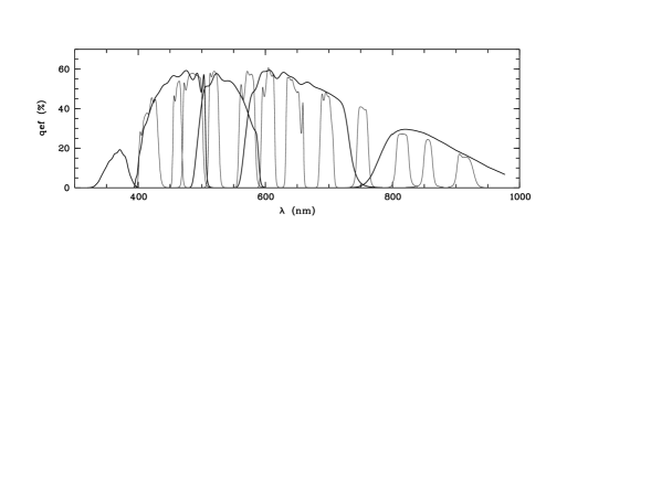
$\lambda_{\mathrm{\mathrm{cen}}}$/fwhm		$t_{\mathrm{\mathrm{exp}}}$	seeing	$m_{\mathrm{\mathrm{lim},10\sigma}}$	run code	mag of Vega	$F_{\mathrm{phot}}$ of Vega
(nm)		(sec)		(Vega mags)		(AB mags)	$(10^{8}\leavevmode\nobreak\ \mathrm{photons/m^{2}/nm/s})$
365/36	$U$	21600	1$\aas@@fstack{\prime\prime}$00	23.9	F, G	$+0.77$	0.737
458/97	$B$	11240	1$\aas@@fstack{\prime\prime}$10	25.1	D, F	$-0.13$	1.371
538/89	$V$	8400	1$\aas@@fstack{\prime\prime}$20	24.5	D	$-0.02$	1.055
648/160	$R$	35700	0$\aas@@fstack{\prime\prime}$75	25.4	D, E, F, G	$+0.19$	0.725
857/147	$I$	9800	1$\aas@@fstack{\prime\prime}$20	22.5	D	$+0.49$	0.412
418/27		7900	1$\aas@@fstack{\prime\prime}$20	24.0	E	$-0.19$	1.571
462/13		10000	0$\aas@@fstack{\prime\prime}$95	24.1	E	$-0.18$	1.412
486/31		5000	1$\aas@@fstack{\prime\prime}$30	23.6	D	$-0.06$	1.207
519/16		6000	1$\aas@@fstack{\prime\prime}$15	23.6	E	$-0.06$	1.125
572/25		4750	0$\aas@@fstack{\prime\prime}$95	23.5	D, E	$+0.04$	0.932
605/21		6000	1$\aas@@fstack{\prime\prime}$00	23.5	E	$+0.10$	0.832
645/30		4000	1$\aas@@fstack{\prime\prime}$15	22.4	D	$+0.22$	0.703
696/21		6000	0$\aas@@fstack{\prime\prime}$90	23.2	E	$+0.27$	0.621
753/18		7000	1$\aas@@fstack{\prime\prime}$00	22.5	E	$+0.36$	0.525
816/21		20000	1$\aas@@fstack{\prime\prime}$00	22.9	E, G	$+0.45$	0.442
857/15		16560	0$\aas@@fstack{\prime\prime}$90	22.0	D	$+0.56$	0.386
914/26		15200	1$\aas@@fstack{\prime\prime}$10	21.9	D, E	$+0.50$	0.380

The COMBO-17 survey has produced multi-colour data in 17 optical filters on 1 $\squareforqed\degr$ of sky at high galactic latitudes. The survey includes the Chandra Deep Field South, centered on the coordinates $\alpha_{2000}=03^{\mathrm{h}}32^{\mathrm{m}}25^{\mathrm{s}}$ and $\delta_{2000}=-27\degr 48\arcmin 50\arcsec$ (see Wolf et al. 2003 for details regarding the other fields). The filter set (Fig. 1 and Tab. 1) contains five broad-band filters (UBVRI) and 12 medium-band filters covering wavelengths from 400 to 930 nm. In this paper, we focus on our observations of the CDFS.

All observations presented were obtained with the Wide Field Imager at the MPG/ESO 2.2m-telescope on La Silla, Chile. The WFI provides a field of view of $34\arcmin\times 33\arcmin$ on a CCD mosaic consisting of eight 2k $\times$ 4k CCDs with at a scale of $0\aas@@fstack{\prime\prime}238$ per pixel. The observations on the CDFS were spread out over four independent observing runs between October 1999 and February 2001. They encompass a total exposure time of $\sim$195 ksec of which $\sim$35 ksec were taken in the R-band during the best seeing conditions.

We needed several observing runs to collect the full 17-filter data set. Hence, for some long-term variable stars and QSOs, the observed 17-passband spectral energy distribution (SED) might be skewed. We attempt to ameliorate the color-independent part of the long-term variability by taking at least R-band data for every observing run, with which we can normalise the SED. We can not correct for variability in colours or for short-term variability on time-scales within an observing run. In addition to long exposures for efficient light gathering, we included short exposures for the photometry of bright objects, in particular to avoid saturation of our brighter standard stars in broad filters.

The long exposures followed a dither pattern with ten telescope pointings spread by $\Delta\alpha$, $\Delta\delta<\pm 72\arcsec$. The pattern allows us to cover the gaps in the CCD mosaic, but also minimises field rotation. Owing to the gaps in the CCD mosaic the total exposure time varies from pixel to pixel. However, the dither pattern makes each position on the sky fall onto a CCD in at least eight of ten exposures, while 97% of all sky pixels are recorded in ten out of ten farmes.

Twilight flatfields were obtained with offsets of $10\arcsec$ between consecutive exposures. Exposure times ranged between 0.5 and 100 seconds per frame. Note that the WFI shutter design allows exposures as short as 0.1 seconds without causing significant spatial variations in the illumination across the CCD mosaic (Wackermann, 1999).

Table 2: COMBO-17 observing runs with CDFS imaging.

run code	Dates
D	07.10.-22.10.1999
E	28.01.-11.02.2000
F	21.09.-30.09.2000
G	19.01.-20.01.2001

We have established our own set of tertiary standard stars based on spectrophotometric observations, mainly in order to achieve a homogeneous photometric calibration for all 17 WFI filter bands. Two stars of spectral types F/G and magnitudes $B_{J}\simeq 16$ were selected in each COMBO-17 field, drawn from the Hamburg/ESO Survey database of digital objective prism spectra (Wisotzki et al., 2000). The spectrophotometric observations for the CDFS were conducted at La Silla on Oct 25, 1999, using the Danish 1.54 m telescope equipped with DFOSC. A wide ($5\arcsec$) slit was used for the COMBO-17 standards as well as for the external calibrator, in this case the HST standard HD 49798 (Bohlin & Lindler, 1992). Two exposures of 45 min were taken of each star, one with the blue-sensitive grism 4 covering the range $\lambda=340$–740 nm, and one with the red-sensitive grism 5 covering $\lambda>520$ nm.

3 Data reduction

3.1 Image reduction and object search

All procedures used for the data reduction are based on the MIDAS package. A WFI image processing pipeline was developed by Wolf et al. (2001) and makes intensive use of programmes developed by K. Meisenheimer, H.-J. Röser and H. Hippelein for the Calar Alto Deep Imaging Survey (CADIS). The pipeline performes basic image reduction and standard operations of bias subtraction, CCD non-linearity correction, flatfielding, masking of hot pixels and bad columns, subtraction of fringe patterns, cosmic ray rejection and subsequent stacking into a deep co-added frame that is common to all dither pointings.

Our deepest co-added frame is the $R$-band image obtained in run D which has a uniform, sharp PSF with $0\aas@@fstack{\prime\prime}75$ FWHM. It provides the most sensitive surface brightness limits and the highest signal-to-noise ratio for object detection and astrometry among all data available in the survey. Only L stars and quasars with $z>5$ have higher S/N in redder bands, a fact which we ignore at this stage. The WFI field of view and the dither pattern lead to a common area of $31\aas@@fstack{\prime}47\times 30\aas@@fstack{\prime}11$ in the $R$-band image.

We used the SExtractor software (Bertin & Arnouts, 1996) with default setups in the parameter file, except for choosing a minimum of 12 significant pixels required for the detection of an object. We first search rather deep and then clean the list of sextracted objects from those having a S/N ratio below 3, which corresponds to $>0\aas@@fstack{m}3123$ error in the total magnitude MAG–BEST. As a result we obtained a catalogue of 63,501 objects in the CDFS, with positions, morphology, total $R$-band magnitude and its error, reaching a 5$\sigma$ point source limit of $R\approx 26$. In this paper, magnitudes are always cited with reference to Vega as a zero point. The astrometric accuracy appears to be better than $0\aas@@fstack{\prime\prime}15$ (see also the comparison with the astrometry from $H$-band imaging by Moy et al., 2003).

3.2 Spectral energy distributions

The spectral shapes of the objects in the $R$-band selected catalogue were measured with a different approach. Photometry in all 17 passbands was done by projecting the object coordinates into the frames of reference of each single exposure and measuring the object fluxes at the given locations. In order to optimize the signal-to-noise ratio, we measure the spectral shape in the high surface brightness regions of the objects and ignore potential low surface brightness features at large distance from the center. However, this implies that for large galaxies at low redshifts $z<0.2$ we measure the SED of the central region and ignore colour gradients.

Figure 2: Errors versus magnitudes for all objects with errors below $0\aas@@fstack{m}1$ in the WFI $U$ and $R$ filter (combined photometry from all epochs).

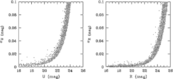
Since seeing variations among the different bands would introduce artificial colour offsets and changing observing conditions are typical for ground-based observations, we need a non-standard photometry approach to measure spectral shapes accurately. In fact, we need to measure the same central fraction of an object in every band as it would appear in equal seeing. To this end, we use the seeing-adaptive, weighted aperture photometry in the MPIAPHOT package (Röser & Meisenheimer, 1991; Meisenheimer et al., 2004).

MPIAPHOT measures the central surface brightness of objects after convolving their appearance outside the atmosphere to an effective PSF of $1\aas@@fstack{\prime\prime}5$ diameter. In detail, the procedure measures the observed stellar PSF on each individual frame and chooses the necessary Gaussian smoothing for reaching a common effective PSF of $1\aas@@fstack{\prime\prime}5$ uniformly on all frames in all bands. For most objects this measurement is similar to a flux measurement in an aperture of $1\aas@@fstack{\prime\prime}5$ diameter in $1\aas@@fstack{\prime\prime}5$ seeing.

The fluxes from individual frames are averaged into a final flux for each object with the flux error being derived from the scatter among the frames. This way, the error does not only take photon noise into account, but also systematic effects, such as suboptimal flatfielding and uncorrected CCD artifacts, which can only be included in the error budget because the object location on the CCD varies with dithering. Also, in this final averaging step we prevent chance coincidences of count rates from pretending unreasonably low errors by using the errors derived from background and photon noise as a lower limit (see Meisenheimer et al., in prep, for a full discussion of the photometric analysis). Furthermore, we do not want transient bad pixels or columns to affect object fluxes, when they are not contained in our bad pixel mask. We eliminate the most outlying single measurement if that reduces the scatter significantly.

3.3 Photometric calibration

The photometric calibration is based on our own spectrophotometric standard stars within the field. We have calibrated these with respect to external standard stars in photometric nights. As a result, we are independent from photometric conditions for all imaging.

The spectra were reduced by standard procedures and have a final signal-to-noise ratio of $>30$ per pixel except very near to the low- and high-wavelength cutoffs. The agreement between spectra in the substantial overlap in wavelength between the two grisms is excellent, confirming that contamination from second order was negligible. We estimated the absolute spectrophotometric accuracy by comparing several spectra of the external calibrator HD 49798 obtained during the entire observing run. The little variation of the overall flux levels indicates that the magnitude calibration is better than 10%. We further estimate that the relative calibration between various wavebands is better than 5%.

The flux calibration for the whole catalogue is then achieved by convolving the spectra of our standard stars with the total system efficiency in our filters. We then know the physical photon flux we have to assign to them, and establish the flux scale for all objects. The validity of the relative calibration, i.e. the shape of the SED, was finally confirmed by comparing the observed stellar locus with its synthetic colours.

Unfortunately, we ended up having only one calibration star in the CDFS, which is furthermore almost located at the edge of the field. The data of the other, more central star in the CDFS turned out to be faulty after the spectroscopic observations were finished. So, the established flux scale relies on object 60873 at $\alpha_{2000}=03^{\mathrm{h}}32^{\mathrm{m}}02\aas@@fstack{s}360$ and $\delta_{2000}=-27\degr 34\arcmin 22\aas@@fstack{\prime\prime}1$. This star of $R\approx 15.5$ matches very well the template of an F5V star from Pickles (1998).

3.4 Variability correction

Since the multi-colour observations were collected over two years and some objects show variability, it was necessary to correct for the latter when constructing the 17-filter spectra for classification. Otherwise, the non-simultaneous SED could mislead the classification about the nature of the object and its photometric redshift. Indeed, the main variable objects are quasars and Seyfert galaxies, but also a few stars and Supernovae superimposed on galaxies. We note, that tests ignoring the variability of quasars have dramatically increased their photometric redshift errors.

Over the entire observing period of COMBO-17 we collected deep $R$-band data so we can measure variability at least in the $R$-band. When constructing the SEDs of variable objects, we relate the measurements of every observed band to the $R$-band magnitude obtained in the same observing run. As a result, the SEDs are not distorted by long-term magnitude changes. This variability correction does not take changes in spectral shape into account, and we also can not correct any short-term variability on the time scale within an observing run as we do not have continuous $R$-band monitoring available.

In search for variability we calculated magnitude differences between any two flux measurements $F_{1}\pm\sigma_{1}$ and $F_{2}\pm\sigma_{2}$ in the same filter

$$\Delta m=2.5\log{F_{1}/F_{2}}\leavevmode\nobreak\ ,$$ (1)

and the associated error

$$\sigma_{\Delta}=\frac{1.085}{\rm{max}(F_{1},F_{2})}\sqrt{\sigma_{1}^{2}+\sigma_{2}^{2}}\leavevmode\nobreak\ .$$ (2)

This comparison was possible for the $R$-band which was observed in all four observing runs, but also in five further bands which were observed twice (see Tab. 1). We take a conservative approach to flagging objects as variable, where we only want to identify genuinely variable objects and avoid contamination by noise spikes. We use a rather high threshold for considering a change significant, because among 60,000 objects we would still expect $\sim 150$ spurious outliers above, e.g., a $3\sigma$ threshold. Also, we are not interested in finding variables among very faint objects, where we can not obtain any redshift estimates, so we used a signal-to-noise cut on the brightness as well. In the end, we only flagged objects as variable when all three of the following criteria were met:

• at least one of the measurements was determined to better than 10$\sigma$, i.e. $\sigma_{1}<0.1$ or $\sigma_{2}<0.1$

• the difference was at least $0\aas@@fstack{m}15$, i.e. $\Delta m>0.15$

• the difference had at least 6$\sigma$ significance, $\Delta m/\sigma_{\Delta}>6$

We applied the variability correction of the SED only for flagged objects. The derived errors of the corrected SED include also the recalibration uncertainties from the $R$-band observations in the various runs. If we applied corrections to all objects, we would increase the total errors in the SED determination of non-variable objects due to the intrinsic error of the correction itself. For objects not fulfilling the variability criteria, we averaged all available measurements in a given filter as measured.

3.5 Flags

The final catalogue contains quality flags for all objects in an integer column, holding the original SExtractor flags in bit 0 to 7, corresponding to values from 0 to 128, as well as some internal quality control flags of our photometry in bits 9 to 11 (values from 512 to 2048). The meaning of SExtractor flags can be found in SExtractor manuals. We generally recommend users to ignore objects with flag values $\geq 8$ (i.e. any bit higher than bit 2 is set), for any statistical analysis of the object population. Their photometry might be affected by various problems, e.g. saturation.

If an object of interest identified in another data source shows bad flags here, it may still have accurate COMBO-17 photometry. Bit 9 indicates only a potential problem (check images for suspicious bright neighbours or reflections from the optics). Higher bits reflect fatal errors: Bit 10 is set when uncorrected hot pixels have severely affected the photometry, and bit 11 was set for some objects we had interactively identified to have erroneous photometry.

4 Classification and redshift estimation

The interpretation of our object SEDs or very-low resolution spectra involves a classification and redshift estimation. It is performed by an automated procedure, as it is the case for any photo-z’s by other authors and for redshift determination in large and modern spectroscopic surveys. A number of authors prefer to reserve the term photo-z to photometry data of low spectral resolution as it is obtained in broad-band surveys. Hence, it would be inappropriate for medium-band redshifts in COMBO-17. Koo (1999), e.g., presented a brilliant review on the subject of photometric redshifts, and proposes to limit the term to imaging data from filters with $\lambda/\Delta\lambda\la 20$.

But the term spectroscopic redshifts would also be unsuitable here. Present-day techniques for constraining redshifts in either photometric or spectroscopic surveys, including COMBO-17, are mathematically all similar. Whether they are applied to 5 passbands, 17 passbands, 500 spectral channels, or even to 2 passbands, makes only a difference in the discriminative power of the data. In the past, we have started to call our medium-band approach by the name fuzzy spectroscopy.

The underlying mathematics of statistical classification procedure have been discussed in WMR. For all details of the technique not explained here, we refer the reader to that source. That work has also modelled surveys with filter sets of different width while keeping the total survey exposure time constant. The results demonstrated that medium-band surveys with less exposure per filter are obviously less deep in terms of object detection than broad-band surveys. But surprisingly they reach to an equal depth in terms of the subsample of objects which are successfully classified and have useful redshift estimates. This means that medium-band surveys produce a similar amount of information as broad-band surveys. At brighter magnitudes, they have the advantage of delivering more information due to the larger number of independent bands, resulting in higher redshift accuracy: a sufficient motivation for the COMBO-17 survey.

4.1 Historical remarks

The idea of photometric redshifts for galaxies dates back to the 1940’s, when Messrs Baade and Hubble initiated a programme to extend tests of cosmological models beyond spectrographic limits and use the potential of the 200” telescope to its photographic limit instead Stebbins & Whitford (1948).

Using photoelectric detectors in nine bands from 350 to 1050 nm and just a single template for elliptical galaxies, Baum (1962) measured redshifts of cluster galaxies out to $z\sim 0.5$ with remarkable accuracy, on the order of $\sigma_{z}<0.02$. His IAU presentation (see discussion in Baum 1962) was met with a mix of encouragement and scepticism. Much that has been said about photo-z’s in the 1950’s and 60’s, still applies today:

• Photo-z’s are controversial: Typically, as redshift estimates they are useful for large samples of objects, but for an individual object they are no proof of its nature.

• Photo-z’s support spectroscopic observations, e.g. when only one line is identified or features are weak and more information is needed.

• Spectroscopic checks are usually appreciated to validate a photo-z sample to ascertain that it is free from systematic errors.

• Systematic errors arising from calibration issues and from mismatch between real spectra and assumed templates are the main limitations to photo-z performance, while aiming for great photon statistics is usually irrelevant.

The redshift accuracies published in the literature have not improved over the last 40 years, but by now the technique is no longer restricted to elliptical galaxies. Therefore, when we say, that photometric redshifts have developed into a mature tool of astronomical information extraction, we mostly mean that they can be more universally applied. Today, photo’zs allow simple spectral classification and even provide redshifts for quasars (Wolf et al., 1999; Budavari et al., 2001).

Photo-z’s are more reliable when more spectral bands are available and when they cover a wider wavelength base. Increasing the wavelength resolution of the filter set increases the redshift accuracy. For a brilliant review on the subject of photometric redshifts, see Koo (1999),

Usually, photometric redshifts are obtained for large object catalogues to provide galaxy or AGN samples for follow-up analysis. Such samples typically spread over a wide range of object magnitudes across which the redshift errors, completeness and contamination change. A simple picture splits the magnitude range into three quality domains, which we specify here for the COMBO-17 survey:

1. the quality saturation domain at $R<22$, where systematic errors from calibration and especially from poor match between templates and true SEDs of celestial objects dominates the performance while the collected photon statistics is irrelevant

2. the quality transition domain at $R=22\ldots 24.5$, where photon statistics take over degrading the performance with decreasing signal

3. the quality breakdown domain at $R>24.5$, where the classification is undecidable using the collected photons and a-priori knowledge of what we should expect dominates the interpretation of the objects completely.

Figure 3: Medium-band power: Pair comparison between objects with similar $BVRI$ colours, where different medium-band SEDs break the degeneracies in broad-band colour diagrams. Multiple error bars mean multiple observations at different epochs. Left panels: A $z=0.67$ galaxy with modest star formation (top) and an M1 star (bottom). Right panels: A $z=2.6$ quasar (top) and an F2 star (bottom).

4.2 Basic technique

One basic technique of photo-zeeing is to use a template database as a model fit to the colour data of an observed object. The templates are arranged into a structured grid with model parameters such as redshift, extinction or SED type. As in any model fit, the model needs to be a good description of the data to yield sensible results, otherwise the statistical test will give a misleading result. So, implicitly we assume that we know of all possible spectra in the universe, and calculate the probability for each of them to produce the colours of an observed object.

The validity of any model fit also depends on the use of correct errors. We emphasize that our method for deriving robust error estimates for each object (see above) is essential to get an accurate statistical confidence for our results, e.g. for the class probabilities and for the estimation of redshift errors of each object itself. We also have to ascertain that there is no mismatch between observed data and template models due to calibration errors. The relative calibration between different passbands is uncertain at a 3% level, and templates may mismatch real SED data at a similar level.

Our template fits do not operate on a linear flux scale but in a colour space of colour indices as detailed in WMR. In order to take calibration tolerances and template mismatch into account we assume a minimum error for each colour index. To this end, we add an error floor of $0\aas@@fstack{m}05$ quadratically to every index error. As in WMR, we calculate explicit colour libraries for a grid in redshift from the spectral libraries before starting any classification code on object catalogues, which saves vast amounts of computing time.

We like to comment on possible other photo-z techniques here: the most relevant alternative to template fitting is based on fitting the empirical colour distributions of galaxies or quasars. This is a valuable approach whenever good model descriptions are unavailable, but there is a large training set of objects with known types and redshifts. It involves either explicit fitting of low-order polynomials Connolly et al. (1995) or implicit fitting as in Artificial Neural Nets (ANNs, e.g. Firth et al., 2003). In our case of a rather deep survey reaching to $z\ga 1$ for galaxies, the classical method of template fitting is currently superior. Once a large number of spectroscopic identifications across all the redshifts become available, ANN approaches will be feasible for COMBO-17 as well.

4.3 Spectral templates

In this subsection we give an update on our current choice of templates over the detailed discussion in WMR.

4.3.1 Star templates

We still take our star templates from the spectral atlas of Pickles (1998), but we restrict it to the spectral types FGKM, because we do not expect any main-sequence OBA stars in this field. Instead we predict from Galactic Halo models that we should find about one Blue Horizontal Branch (BHB) star, several white dwarfs and possibly blue (sdB) subdwarfs. For the latter, we introduced a new class for blue high-gravity stars using synthetic templates by Koester (priv. comm.), effectively matching colours of white dwarfs and sdB subdwarfs, but also matching BHB stars in the low-$g$ domain. From Koester’s grid of atmosphere models we select the DA dwarf models in the temperature range from 6,000 K to 40,000 K and the surface gravity range of $\log g=6.0\ldots 9.0$.

Figure 4: Galaxy redshifts old and new: The change-over in the template set for galaxies has changed the redshifts of most galaxies relatively little. But it has improved the overall redshift accuracy and also the completeness in redshift determination.

4.3.2 Galaxy templates

The galaxy template library used in our team has been completely rebuilt and contains now a grid of synthetic spectra based on the PEGASE code Fioc & Rocca-Volmerange (1997) for population synthesis models. In the past, we used the observed templates by Kinney et al. (1996), which where still used for the work on the evolution of the galaxy luminosity function (Wolf et al. 2003a).

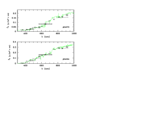
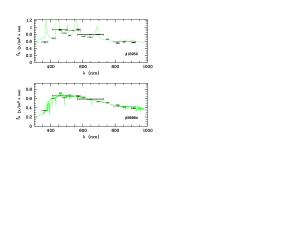
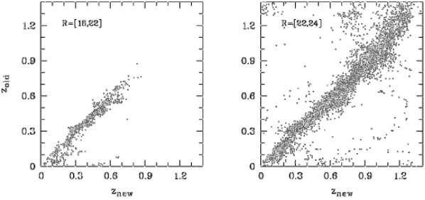
We found that the new templates deliver a better redshift accuracy than the old ones. The changes in redshift are relatively small as demonstrated in Fig. 4 and within the errors of the old redshift estimates. But the residual errors have been reduced in the new optimised redshifts and allow unprecedented photo-z accuracy. The resulting luminosity functions of galaxies are unchanged within the errors published in Wolf et al. (2003a). The luminosity functions of red-sequence galaxies published by Bell et al. (2004) are already based on the new redshifts.

The new grid includes the full range of the Kinney templates, and actually covers a wider range of spectral types, extending to slightly bluer and redder spectra. Further advantages of the synthetic spectra are the more regular grid in spectral types, the more physical parametrization of the types and the possibility to extend the grid into more than just one dimension given by a single type parameter.

The templates span a two-dimensional grid with a range of ages calculated by the PEGASE code and a range of extinction levels which we applied as external screens to the SEDs delivered by PEGASE. The setup for PEGASE uses standard parameters suggested by the codes SSPs and scenarios with a Kroupa (1993) IMF and no extinction. The star formation history follows an exponential decay law with a time constant of $\tau=1$ Gyr. The SEDs are calculated by PEGASE for various time steps since the beginning of the first star formation. As templates we use 60 spectra for look-back times (”ages”) ranging from 50 Myr to 15 Gyr.

We tune initial model metallicities to give almost solar metallicity over the whole range of templates. This reproduces approximately the metallicity of the L* galaxies which dominate any magnitude-limited sample. It is worth noting, however, that the well-known age/metallicity degeneracy is actually helpful in this case: Mismatches between real galaxy and template galaxy metallicities can be compensated for by modest changes in template age, while yielding nonetheless accurate estimates of redshift and SED shape.

The COMBO-17 classifier also allows for dust reddening. The COMBO-17 photometry of galaxies with known redshift $z>0.6$ shows little sign of an absorption trough near restframe 220 nm. In contrats, a Milky Way-type extinction law has a strong 220nm trough, and hence we do not adopt such a reddening law for our templates. We experimented with the well-known Calzetti law, but it seemed to produce insufficient curvature between 180 and 400 nm to match our observations. We have found a satisfactory ad-hoc solution using the 3-component extinction law by Pei (1992). We decided to use his SMC law, because it provided a reasonably good match between templates and observed SEDs of galaxies with previously known redshift. The issue of dust extinction certainly deserves a more thorough exploration, for which COMBO-17 could supply a wealth of photometric data. However, we defer this issue to a future work. Note, that the detailed choice of extinction law has no effect on the observed SEDs of galaxies with $z<0.6$. All templates are then extinguished with six different equidistant degrees of reddening in the interval of $E_{B-V}=[0.0,0.1,...0.5]$.

The redshift grid for the galaxy colour library covers the range from $z=0$ to $z=1.40$ in 177 steps. These are equidistant on a $\log(1+z)$ scale with steps of 0.005 and of course limit the redshift resolution when reconstructing galaxy density features in redshift space. According to the sampling theorem, features in redshift space can be recovered if their wavelength is at least as large as two grid steps. Thus, we have to expect that features with wavelength $\delta_{z}/(1+z)<0.01$ will be smoothed by our redshift estimation even under perfect conditions where systematic problems in photometric calibration or SED match are absent. This will not significantly restrict the power of our dataset, because our redshift estimation is probably not consistently much more accurate than 0.01 across all redshifts and SEDs we are interested in.

4.3.3 QSO templates

The QSO template library is derived from the SDSS template spectrum vanden Berk et al. (2001). This template resembles a typical emission line contour on top of an average QSO continuum. In order to cover the range of SEDs expected for QSOs, we generated spectra of different continuum slope and emission line strength. For this purpose, we have varied the given template in intensity and added it to a power-law continuum. We do not need to vary the relative strength of different emission lines by much, since the filter set usually shows one, or sometimes two, emission lines in the medium-band filters. Finally, we have taken the Hydrogen absorption bluewards of the Lyman-$\alpha$ line into account by multiplying intrinsic SEDs by a redshift-dependent throughput function Møller & Jakobsen (1990).

The effective spectral indices of the resulting spectra depend on redshift since the continua are not power laws. The observed $B-I$ colour of the QSO templates at $z=2$ runs from about +0.35 to +1.75 (in Vega magnitudes), corresponding roughly to power law indices from $\alpha=-1.66$ to $+0.4$. The final colour library covers QSO redshifts across $z=[0.5,5.96]$. At $z<0.5$, the template does not cover the full COMBO-17 filter set, so that the fits would be less constrained than at other redshifts. Hence, the classifier is insensitive to QSOs at $z<0.5$. In fact, we expect very few such objects, and chose to ignore the problem. The library grid has 20 steps in the spectral slope axis, nine steps in emission line strength and 155 steps in redshift with a resolution of 0.01 in $\log(1+z)$. Hence, features in $z$ space smaller than $\delta_{z}/(1+z)=0.02$ are smoothed, but we do not intend to study such substructure in the small QSO sample, anyway.

Figure 5: Template fit – histograms of reduced $\chi^{2}$ values: Left panel: At bright levels of $R=[18,22]$ photon noise is irrelevant. The quality of template fits is limited by calibration errors and template variety. The $\chi^{2}$ values scatter a bit higher than expected. Right panel: For fainter objects, flux errors from photon noise dominate the template fits. Hence, they show very much the expected $\chi^{2}$ distribution.

4.4 Classification rules

First, the probability of each template producing the observed colours of a given object is calculated on the basis of the match quality and the photometric errors. Then, its actual classification involves a decision between the basic alternatives Star, WDwarf, Galaxy and QSO. Therefore, we compare the integrated probabilities of each of the four classes, after normalising their sum to 100% to indicate our assumption that no further class may exist.

Before the decision is made, we multiply each class probability with the a-priori probability of an object to belong to any of the classes depending on its observed magnitude (in the I-band). Hence, we have used all the available photometric information for the classification. The first step of template comparison uses only colour indices or spectral shapes, but in the second step the overall brightness (i.e. the free normalisation parameter in template fitting) is factored into the probabilities via a-priori class distributions. These a-priori functions are simple linear approximations of our number counts. At the faintest levels, where the classification breaks down, the number counts are uncertain, and the linear fits probably don’t reflect the true distribution.

As in WMR, a decision is made in favour of a single class if it accounts for $>75$% of the total probability. At $R<23$, around 90% of the objects are classified with a probability of $>99$% focussed on one class interpretation, suggesting a 1-in-100 risk for misclassifications among these. The other 10% are less clear cases, and reside in parts of the colour space where templates from more than one class crowd together, implying the filter set is not sufficient to discriminate between them unambiguously. A decision based on 75% probability in favour of one class translates into a 1-in-4 chance that the wrong class has been assigned! We assign Galaxy (Uncl!) to unclassified objects below the 75% margin, reflecting that the decision is very uncertain. Most often, these objects are galaxies anyway, because the linear number count fits used by us tend to overestimate the density of stars and QSOs at faintest levels. In any case, it will be the safest approach to count those in the rich Galaxy class if anywhere. Some true stars and QSOs will be in this group, but they do not form a significant fraction of contaminants given how dominant galaxies are at faint magnitudes (see also discussion on contamination in Sect. 7.3).

There are a few conditions, under which we override this statistical approach with hard rules:

Faint stars at the red end of the WDwarf grid or on the blue end of the Pickles FGKM sequence should be classified either as Star or WDwarf. But their large photometric errors can result in high probabilities just below 50% for both classes, and we do not want them to be labelled Galaxy (Unclassified). So, if $p(Star)+p(WDwarf)>75$% we still assign the more probable one of the two stellar classes with no further comment.

A second non-statistical rule is applied for objects with point-source morphology and classification as galaxies with $z<0.2$. Noisy photometry leaves faint galaxies at redshifts near zero difficult to differentiate from stars and sometimes causes their misclassification as stars. In case of a clearly extended morphology, we override the probability-based classification and set the class to Galaxy (Star?), indicating that usually we are looking at misclassified galaxies here, but as a second guess we might really be looking at a resolved stellar binary.

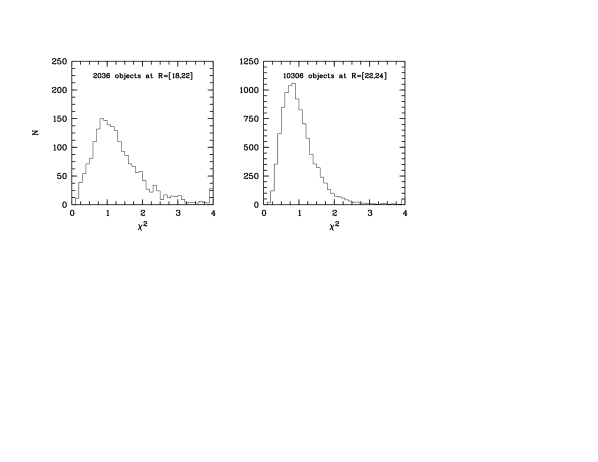
The great majority of objects match our templates rather well. Histograms of reduced $\chi^{2}$ values for the best fitting templates show maxima around 1.0, just as it is desired statistically (see Fig. 5). Objects with reduced $\chi^{2}$ values $>30$ are simply classified as Strange Object whatever their probabilities for different classes are. These objects are highly inconsistent with all existing templates and many have bad flags anyway. Some of them are clearly real objects with accurate photometric data, but unusual spectra, e.g. galaxies with extremely strong emission lines or objects with strong variability on a time scale of hours or days. For statistical studies of the bulk object population we suggest to ignore them, but if your pet object is among them, our data could still be useful (depending on the flags).

Figure 6: Estimated redshift errors: Redshift error vs. redshift (left panel) and vs. $R$-band magnitude (right panel) for 10,041 galaxies with MEV redshift estimates. The errors are driven by photon noise. At $z\sim 1$ hardly any galaxies are measured with errors below 0.02, because only few of them are sufficiently bright.

Figure 7: Bimodal redshift solutions: Left panel: $R$-band histogram of all galaxies with MEV redshift estimates and a subset of those having bimodal probability distributions for their photometric redshift. At $23<R<24$, 20% of all galaxies have a bimodal $p(z)$. Right panel: Alternative (less likely) redshift vs. assigned (more likely) redshift for $\sim 1350$ galaxies with bimodal $p(z)$ at $R<24$.

4.5 Photometric redshifts

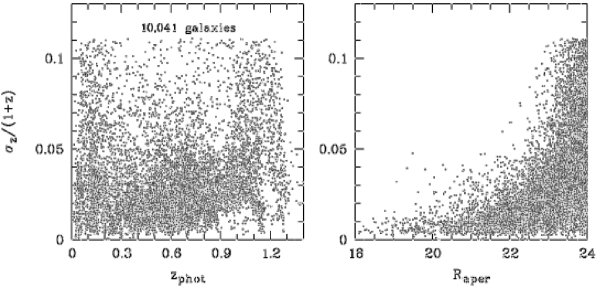
As in WMR, we compress the information of the full redshift probability distribution $p(z)$ of an object into a few numbers. These are the actual redshift estimate and its estimated error. Such a simplified approach is fine as long as $p(z)$ looks similar to a Gaussian or is at least not widely distributed. Our estimator of choice is the Minimum-Error-Variance (MEV) estimator also known as Mean-Square (MS) estimator, which calculates just the mean and variance of the $p(z)$ distribution. By definition, it minimises the average true deviation of estimates in a sample. The magnitude dependence of redshift errors in the galaxy sample (see Fig. 6) demonstrates how these errors are driven by photon noise.

Whenever probability distributions are not well represented by a single Gaussian, a small set of numbers like mean and variance can not convey its more complex structure and may be misleading. A common situation in photometric redshift determination involves bimodal $p(z)$ functions that are just the sum of two Gaussians centered at different redshifts. These cases are the result of ambiguities in colour space, where the filter set does not discriminate between alternative interpretations.

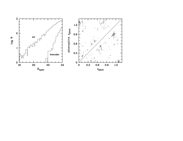
Our algorithm detects bimodal cases and compares the probability integral under the two modes to decide for the more likely alternative. We then list mean and variance of the more likely mode, but we also set a flag for bimodality and list a second-guess redshift from the other mode. In the quality saturation domain, the SED is defined clearly enough to avoid any ambiguities. In the quality transition domain bimodal cases amount to 4% of all galaxies at $R=[22,23]$ and 20% of those at $R=[23,24]$ (see Fig. 7 for a magnitude histogram and the alternative redshifts).

If the $p(z)$ distribution is rather wide, mode decomposition will not make much sense anymore, and storing the full distribution would enlarge the data volume beyond our intention. Also, the COMBO-17 data confront us with this situation only at $R>23.5$, where the classification might be inaccurate in either case. This is because it faces a number of systematic challenges beyond the problem of increased noise, such as our restriction in galaxy templates and redshifts and the lack of observed NIR data. For the same reason, we do not use redshift priors depending on apparent magnitude. At $R<23$ such priors are virtually irrelevant compared to the narrow colour-based $p(z)$ distributions and would not add information. At fainter levels they are relevant, but priors could not fix the damage caused by all the limitations of restframe UV galaxy templates.

We like to briefly comment on how to deal with wide $p(z)$ distributions in hypothetical applications. The MEV estimator will still give the best estimate for individual objects if a compression into a single number is desired. Of course, for a flat $p(z)$ this will always be the central redshift of the interval probed, but the average deviation of a sample will still be minimised to $\sqrt{1/3}$ of the full interval width. But plotting a histogram of redshifts thus obtained will be a misleading exercise, because after the compression of $p(z)$ into a single number any distribution information has been erased. Reconstructing a best estimate of the redshift distribution for all objects combined requires summing up the original $p(z)$ distributions.

We decided not to use any MEV estimates, whenever the 1-$\sigma$ error exceeded a threshold chosen ad-hoc to be 1/8 of the full redshift interval in grid space. This translates to an estimated redshift error threshold which is constant in $\sigma_{z}/(1+z)$ due to the changing grid constant in redshift space (see also Fig. 6).

4.6 Known deficiencies

The classification procedure contains three principal ingredients. The first one is the data, largely characterized by the choice of filters and exposure times. The second ingredient is the model, or equivalently our template set. Finally, the third ingredient is the classifier, which may include priors and non-statistical rules.

Our choices on all three ingredients influence the classification quality on the whole. The filter set leaves room for some class ambiguities, which COMBO-17 can not resolve on its own and which lead to misclassifications. Our simulations of the survey provide us not only with completeness maps, but also with class cross-contamination maps, which can point to the most relevant issues (see Sect. 7.3). Also, any template set will always be incomplete and can not be expected to catch every object we come across. In the following, we highlight some limitations of the classification we are aware of.

Binary stars: The stellar library contains no ”M dwarf plus White Dwarf” binaries, which have colours that are inconsistent with any single star template because of the comparable brightness of the two components. These binaries are often serendipitously found in searches for QSOs by optical colour.

Extremely cool stars: The stellar library contains no L dwarf spectra, which are not much redder than M dwarfs in optical colours but have weaker absorption bands. Their extremely low luminosity should render them invisible in our sample, and the brightest and warmest examples of type L0/1 might still be matched reasonably well with the Pickles M8 template.

High-redshift galaxies: Galaxies at $z>1.3$ show no distinctive features in our filter set and are typically quite faint. Both factors suggest that these galaxies are mapped onto a rather broad $p(z)$ distribution, and it should be almost impossible to obtain accurate redshift information from COMBO-17. We truncated the probability determination of galaxy redshifts at $z=1.4$ and deliberately excluded higher redshift galaxies from the scope of our work. At this point, we can not tell what really happens to these galaxies in COMBO-17, because we are lacking a suitable spectroscopic control sample. In principle, it is possible that these objects will contaminate the low-z sample, if a well constrained but random match with low-z templates occurs. But it is more likely, that $z>1.3$ galaxies are found among those with no MEV redshifts.

To test the plausibility of this assumption, we now estimate the number of expected high-z objects and compare it with the number of objects without redshifts. Virtually all $z>1.3$ galaxies are at $R>23$, while objects at $R>24$ are not within the scope of COMBO-17. Hence, we inspect the interval of $R=[23,24]$, where we have a total of $\sim 7300$ galaxies. Baugh & Efstathiou (1991) provide an approximate redshift distribution as a function of median sample redshift. Using this result with the median redshift $z_{m}=0.75$ measured by Brown et al. (2003) for COMBO-17 in the interval $R=[23,24]$, we anticipate that 10% of objects in this interval should lie at $z>1.3$. However, we find that 17.5% of objects in this interval have no MEV redshifts due to a broad p(z) distribution. It is hence possible, that all the high-z galaxies hide among those with no redshift estimate. However, even if many of the relatively rare high-z objects had been mistakenly assigned a low redshift, we believe they would not compromise the value of the rich low-z sample.

Seyfert-1 galaxies: Seyfert-1 galaxies are detected as QSOs provided their active nucleus is sufficiently luminous compared to the stellar light of the host galaxy, such that the nucleus leaves significant signature in the 17-filter SED. Typically, broad-line AGN brighter than $M_{B}=-21.7$ are identified as AGN and are tagged QSO. Fainter broad-line objects are only sometimes recognized as QSO, but mostly just classified as Galaxy. At $z>1$ the redshifts of AGN classified as Galaxy are unreliable, and the full catalogue could contain up to a few dozen such objects.

Seyfert-2 galaxies: Many galaxies belong to the Sy-2 class and can be identified as such in deep X-ray observations, but the wavelength resolution of COMBO-17 does not allow to tell the difference to normal galaxies, because we can not clearly see the emission lines. Hence, the AGN nature of these galaxies is usually not discovered by COMBO-17, while their redshifts should be as reliable as those of normal galaxies.

Compact low-z galaxies: At $z<0.2$ and fainter magnitudes, where photometry is less accurate, some galaxies show very similar colours as stars even in 16-D colour space. We break this degeneracy using morphological information. However, very faint and unresolved low-z galaxies could still be mistaken as stars, and slightly resolved binaries could then be misclassified as galaxies. At present we have no idea, how common this mistakes could be, but we estimate that at most it should be a few dozen objects at $R<24$.

4.7 Derived restframe properties

The restframe luminosity of all galaxies and quasars are measured from the individual 17-filter spectra. For the galaxies, ten restframe passbands are considered, SDSS $ugr$ bands, $UBV$ bands in Johnson and Bessell systems and a synthetic UV continuum band centered at $\lambda_{\mathrm{rest}}=280$ nm with 40 nm FWHM and a top-hat transmission function. For quasars, we give luminosities in a synthetic rectangular passband at 140 nm–150 nm. Depending on the restframe band and the redshift in consideration, these luminosities are sometimes based on extrapolations beyond our filter set. In these cases, the values as well as their estimated errors tend to be uncertain. At higher redshift, our filter set probes the restframe UV spectrum which is dominated by light from the youngest population in a galaxy. Older populations could be hidden in the restframe UV signal, and only contribute to restframe visual light. These would not be constrained by the observed SED, but could strongly affect the visual restframe passbands.

We derive restframe luminosities by placing the redshifted template that corresponds to the galaxy SED into the observed 17-band photometry. Then we integrate the template spectrum under redshifted versions of the restframe passbands. Our reddest restframe band, the SDSS $r$-band, requires extrapolation at all redshifts $z>0.5$. The most ultraviolet band, 280/40, is extrapolated at low redshifts of $z<0.25$. Tab. 3 lists all extrapolation-free redshift ranges. For quasars, we directly measure restframe luminosities over $1.4<z<5$ without any extrapolation. In Tab. 5 we give reference data for all restframe passbands. We would like to ask the user not to trust restframe colours for galaxies at $z>1.1$ too much, because there (a) most passbands are extrapolated and (b) increasing errors in redshift propagate into the restframe quantities. We have not modelled the errors introduced by either effect.

At least, we have estimated errors for the luminosities from the errors of the observed photometry. These should be reasonable error estimates in the non-extrapolation regimes. We add the following three error components in quadrature: (i) the magnitude error of the broad-band filter closest to the redshifted restframe passband, because it determines the local flux level in the passband relative to the whole SED; (ii) the magnitude error of the total magnitude MAG-BEST, because it determines the overall flux level for the whole object; and (iii) a minimum error of $0\aas@@fstack{m}1$ to take into account various contributions from redshift errors or from the overall calibration.

We would like to remind the reader of two additional, important sources of error for luminosities which we have not taken into account. Firstly, whenever redshifted restframe passbands lie outside the observed filter set, the luminosity estimate relies on an extrapolation of the SED as it has been fit within the filter set. But true SEDs can deviate from best-fitting ones, e.g. when an underlying older population shows up in the observed NIR regime, but is invisible in the observed visual and leaves no trace in the template then. The reader may be warned that our luminosities are then only rough estimates. Secondly, large galaxies at low redshifts show only their central colours in our apertures used for the SED measurement. Hence, colour gradients inside the galaxy will not be properly reflected in the galaxy luminosities. Only in the observed-frame $R$-band, the total galaxy photometry is correct. All other bands are linked to this measurement through the SED shape measured in apertures. Colour gradients would affect all luminosities where restframe passbands are far away from the observed $R$-band. Throughout the paper, we use $H_{0}=h\leavevmode\nobreak\ \times$ 100 km/(s Mpc) in combination with $(\Omega_{m},\Omega_{\Lambda})=(0.3,0.7)$.

Table 3: Column entries in the published FITS catalogue. For details of the ASCII version, see CDS or COMBO website. Some restframe luminosities are extrapolated in some redshift ranges. We give the redshift intervals, where no extrapolation errors are expected.

column header meaning general information Nr unique object number ra right ascension (J2000) dec declination (J2000) x x-position on $R$ frame in pixels y y-position on $R$ frame in pixels Rmag total $R$-band magnitude e_Rmag 1-$\sigma$ error of total $R$-band mag Ap_Rmag aperture $R$-band magnitude in run D ApD_Rmag difference total to aperture (point sources $\sim 0$) mu_max central surface brightness in $R$ from SExtractor MajAxis major axis (as observed in $1\arcsec$ seeing) MinAxis minor axis (as observed in $1\arcsec$ seeing) PA position angle, measured West to North phot_flag photometry flags (see Sect. 3.5) var_flag variability flag (0 = not variable) stellarity stellarity index from Sextractor classification results MC_class multi-colour class (see Tab. 4) MC_z mean redshift in distribution $p(z)$ e_MC_z standard deviation (1-$\sigma$) in distribution $p(z)$ MC_z2 alternative redshift if $p(z)$ bimodal e_MC_z2 standard deviation (1-$\sigma$) at alternative redshift MC_z_ml peak redshift in distribution $p(z)$ chi2red $\chi^{2}/N_{f}$ of best-fitting template dl luminosity distance of MC_z total object restframe luminosities UjMag $M_{abs,gal}$ in Johnson $U$ (ok at all $z$) e_UjMag 1-$\sigma$ error of $M_{abs,gal}$ in Johnson $U$ BjMag $M_{abs,gal}$ in Johnson $B$ ($z\approx[0.0,1.1]$) e_BjMag 1-$\sigma$ error of $M_{abs,gal}$ in Johnson $B$ VjMag $M_{abs,gal}$ in Johnson $V$ ($z\approx[0.0,0.7]$) e_VjMag 1-$\sigma$ error of $M_{abs,gal}$ in Johnson $V$ usMag $M_{abs,gal}$ in SDSS $u$ (ok at all $z$) e_usMag 1-$\sigma$ error of $M_{abs,gal}$ in SDSS $u$ gsMag $M_{abs,gal}$ in SDSS $g$ ($z\approx[0.0,1.0]$) e_gsMag 1-$\sigma$ error of $M_{abs,gal}$ in SDSS $g$ rsMag $M_{abs,gal}$ in SDSS $r$ ($z\approx[0.0,0.5]$) e_rsMag 1-$\sigma$ error of $M_{abs,gal}$ in SDSS $r$ UbMag $M_{abs,gal}$ in Bessell $U$ (ok at all $z$) e_UbMag 1-$\sigma$ error of $M_{abs,gal}$ in Bessell $U$ BbMag $M_{abs,gal}$ in Bessell $B$ ($z\approx[0.0,1.1]$) e_BbMag 1-$\sigma$ error of $M_{abs,gal}$ in Bessell $B$ VbMag $M_{abs,gal}$ in Bessell $V$ ($z\approx[0.0,0.7]$) e_VbMag 1-$\sigma$ error of $M_{abs,gal}$ in Bessell $V$ S280Mag $M_{abs,gal}$ in 280/40 ($z\approx[0.25,1.3]$) e_S280Mag 1-$\sigma$ error of $M_{abs,gal}$ in 280/40 S145Mag $M_{abs,QSO}$ in 145/10 ($z\approx[1.4,5.2]$) e_S145Mag 1-$\sigma$ error of $M_{abs,QSO}$ in 145/10 observed seeing-adaptive aperture fluxes W420F_E photon flux in filter 420 in run E e_W420F_E photon flux error in 420/E W462F_E photon flux in filter 462 in run E e_W462F_E photon flux error in 462/E column header meaning observed seeing-adaptive aperture fluxes (cont.) W485F_D photon flux in filter 485 in run D e_W485F_D 1-$\sigma$ photon flux error in 485/D W518F_E photon flux in filter 518 in run E e_W518F_E 1-$\sigma$ photon flux error in 518/E W571F_D photon flux in filter 571 in run D e_W571F_D 1-$\sigma$ photon flux error in 571/D W571F_E photon flux in filter 571 in run E e_W571F_E 1-$\sigma$ photon flux error in 571/E W571F_E photon flux in filter 571 combined e_W571F_E 1-$\sigma$ photon flux error in 571/combined W604F_E photon flux in filter 604 in run E e_W604F_E 1-$\sigma$ photon flux error in 604/E W646F_E photon flux in filter 646 in run D e_W646F_E 1-$\sigma$ photon flux error in 646/D W696F_E photon flux in filter 696 in run E e_W696F_E 1-$\sigma$ photon flux error in 696/E W753F_E photon flux in filter 753 in run E e_W753F_E 1-$\sigma$ photon flux error in 753/E W815F_E photon flux in filter 815 in run E e_W815F_E 1-$\sigma$ photon flux error in 815/E W815F_G photon flux in filter 815 in run G e_W815F_G 1-$\sigma$ photon flux error in 815/G W815F_S photon flux in filter 815 combined e_W815F_S 1-$\sigma$ photon flux error in 815/combined W856F_D photon flux in filter 856 in run D e_W856F_D 1-$\sigma$ photon flux error in 856/D W914F_E photon flux in filter 914 in run E e_W914F_E 1-$\sigma$ photon flux error in 914/E UF_F photon flux in filter U in run F e_UF_F 1-$\sigma$ photon flux error in U/F UF_G photon flux in filter U in run G e_UF_G 1-$\sigma$ photon flux error in U/G UF_S photon flux in filter U combined e_UF_S 1-$\sigma$ photon flux error in U/combined BF_D photon flux in filter B in run D e_BF_D 1-$\sigma$ photon flux error in B/D BF_F photon flux in filter B in run F e_BF_F 1-$\sigma$ photon flux error in B/F BF_S photon flux in filter B combined e_BF_S 1-$\sigma$ photon flux error in B/combined VF_D photon flux in filter V in run D e_VF_D 1-$\sigma$ photon flux error in V/D RF_D photon flux in filter R in run D e_RF_D 1-$\sigma$ photon flux error in R/D RF_E photon flux in filter R in run E e_RF_E 1-$\sigma$ photon flux error in R/E RF_F photon flux in filter R in run F e_RF_F 1-$\sigma$ photon flux error in R/F RF_G photon flux in filter R in run G e_RF_G 1-$\sigma$ photon flux error in R/G RF_S photon flux in filter R combined e_RF_S 1-$\sigma$ photon flux error in R/combined IF_D photon flux in filter I in run D e_IF_D 1-$\sigma$ photon flux error in I/D

5 Published data

The published data package includes the object catalogue and coadded images in the five broad bands of COMBO-17. They are all available from CDS or at the COMBO-17 website (http://www.mpia.de/COMBO/combo_index.html). From the latter site the catalogue is available in both FITS and ASCII format. Given the large number of data columns the FITS version is probably the most trivial one to use in practice. However, we provide an ASCII table for users who can not read FITS tables (see the COMBO-17 website for notes on how to read FITS tables most easily in IDL or MIDAS).

The catalogue lists identifiers, positions, magnitudes, morphologies, as well as classification and redshift information as detailed in Tab. 3. All magnitudes given in the catalogue and this paper use a spectrum of Vega as their zeropoint, even for filters traditionally defined in an AB system (e.g., SDSS $u$, $g$, and $r$). This is also true for all the restframe luminosities. If readers prefer AB magnitudes, a conversion has to be made based on Vega values given in Tab. 1 and Tab. 5. Magnitude values such as the total apparent $R$-band magnitude $Rmag$ and all luminosities are total object magnitudes based on the SExtractor definition of $MAG\_BEST$. In contrast, the observed filter flux values are all seeing-adaptive aperture fluxes and are calibrated such that they are equal to total fluxes for point sources. An exception among the magnitudes is the $R$-band aperture magnitude from run D, $Ap\_Rmag$, which is just the Vega magnitude corresponding to the flux $RF\_D$. Fluxes are given as photon fluxes $F_{\mathrm{phot}}$ in units of photons/m²/s/nm. Photon fluxes are related to other flux definitions by

$$\nu F_{\nu}=hcF_{\rm phot}=\lambda F_{\lambda}\leavevmode\nobreak\ .$$ (3)

Photon fluxes are rather practical units at the depth of current surveys. A magnitude of $V=20.0$ corresponds to 1 photon/m²/s/nm in all systems (AB, Vega, ST), if $V$ is centered on 548 nm. When the band flux of an object is missing, it means that every exposure was saturated in this band.

The column $ApD\_Rmag$ contains the magnitude difference between the total object photometry and the point-source calibrated, seeing-adaptive aperture photometry:

$$ApD\_Rmag=Rmag-Ap\_Rmag\leavevmode\nobreak\ .$$ (4)

On average, this value is by calibration zero for point sources, and becomes more and more negative for extended sources of increasing size.

The $var\_flag$ column reports the number of flux comparisons between multiple observations of identical bands, where an object has been found as variable. This number is 0 for objects with no such variability, and up to 8 for objects which have been found as variable in all the eight available comparisons.

The coadded images are provided as FITS images and have slightly different coordinate systems. The $U$-band image is rotated with respect to the four others, because in February 2000 the WFI camera was serviced and mounted back to the telescope in a slightly different orientation. Hence the pixel coordinates of any given object can differ on the $U$ image by up to five pixels from the other bands. The images are $7951\times 7595$ pixels in size and cover the area common to the $BVRI$ frames. The $U$-band frame has the same format although 115 columns ($<30\arcsec$) at the left edge are blank due to pointing differences. The instensity levels of the images are given in units of photons hitting the detector, so the CCD gain is taken out. We strongly recommend readers to use the known spectrophotometric standard star for calibration in case they obtain their own independent photometry.

Table 4: Definition of entries for the mc_class column.

class entry	meaning
Star	stars
	(colour of star, stellar shape)
WDwarf	WD/BHB/sdB star
	(colour of WD/BHB/sdB, stellar shape)
Galaxy	galaxies
	(colour of galaxy, shape irrelevant)
Galaxy (Star?)	most likely galaxy at $z<0.15$
	(but overlap in colour space with stars)
Galaxy (Uncl!)	colour undecided
	(statistically almost always a galaxy)
QSO	QSOs
	(colour of QSO, stellar shape)
QSO (Gal?)	colour of QSOs, extended shape
	(usually Seyfert, but maybe contaminating galaxy)
Strange Object	very strange spectrum
	(unusual intrinsic spectrum, strong photometric
	artifacts or uncorrected strong variability)

Table 5: The restframe passbands and their characteristics.

name	$\lambda_{\mathrm{\mathrm{cen}}}$/fwhm	mag of Vega	$F_{\mathrm{phot}}$ of Vega
	(nm)	(AB mags)	$(10^{8}\leavevmode\nobreak\ \mathrm{phot/m^{2}/nm/s})$
(synthetic)	145/10	$+2.33$	0.447
(synthetic)	280/40	$+1.43$	0.529
Johnson $U$	365/52	$+0.65$	0.820
Johnson $B$	445/101	$-0.13$	1.407
Johnson $V$	550/83	$+0.00$	1.012
SDSS $u$	358/56	$+0.84$	0.704
SDSS $g$	473/127	$-0.11$	1.305
SDSS $r$	620/115	$+0.14$	0.787
Bessell $U$	361/65	$+0.71$	0.780
Bessell $B$	441/95	$-0.13$	1.415
Bessell $V$	551/85	$+0.00$	1.009

Figure 8: Left panel: Star sample: $B-V$ colour vs. $R$-band magnitude. Variable stars are marked by a circle. Right panel: Galaxy sample: MEV redshift estimate vs. $R$-band magnitude (black: red sequence galaxies, grey: star-forming galaxies).

Figure 9: Galaxy sample: Restframe $280-B$ colour vs. $M_{B}$ luminosity. The sharp sample cutoff on the right corresponds to $R=24$, the most reliable subsample. The distribution is clearly bimodal, with a red sequence and a blue cloud of star-forming galaxies.

Figure 10: Galaxy sample: Redshift histogram from MEV estimates at magnitude limits of $R<23$ (black line) and $R<21$ (grey line). The redshift distribution in the CDFS is clearly unusual and not representative of the cosmic average. The redshifts themselves are quite reliable as the comparison in Sect. 8 shows.

Figure 11: Quasar sample: Left panel: Redshift vs. $R$-band magnitude for all identified quasars with MEV redshift estimates. Right panel: The purely optical COMBO-17 selection of type-1 AGN is basically complete at luminosities $M_{B,{\rm Vega}}<-21.7$ (solid line), where nuclear light contributes significantly to the SED. At lower AGN luminosities the SED is dominated by stellar light from the host galaxy. Shown here are all type-1 AGN identified in X-ray follow-up of the CDFS 1 Msec image. Large circles mark those identified in COMBO-17 as quasars, and small dots those classified as normal galaxies – their AGN nature can only be discovered with X-rays or spectroscopy.

6 Classified object samples

Most work done with the catalogue will either be the selection of samples according to some criteria, e.g. ’all stars’, ’all QSOs at $z>2$’ or be the identification of sources with known position, e.g. X-ray counterparts. However, for the characterization of the data we present some figures which can immediately be plotted from the published catalogue. We give some sample queries below, where we also use wildcards (*) when selecting objects by class name. These queries will mostly address the magnitude range from $R=16$ to $R=24$ in terms of the aperture magnitude $Ap\_Rmag$. Brighter than $R=16$ some flux measurements are saturated and the SED is potentially incomplete. Faintwards of $R=24$ the completeness and reliability of the redshifts and classifications drop too far down.

Figure 12: Three objects at R=[16,24] were classified as Strange Object based on their remarkably poor fits to all available templates (see text for more details).

6.1 Stars and ’WDwarfs’

A query for $MC\_class=^{\prime}Star*^{\prime}$ and $16<Ap\_Rmag<24$ selects 997 objects from the catalogue. Five of them have bad flags ($phot\_flag>7$), but their photometry looks fine to us. At $R<16$, stars are saturated in the deep $R$-band stack and get the saturation flag in the catalogue. Most filters were observed with additional short exposures providing a flux measurement where saturation prevents it (unfortunately not the $R$-band in run D). Hence, most aperture photometry (calibrated to resembe full magnitude for point sources anyway) should be fine when measurements appear in the catalogue. The final saturation limits range from $m\sim 12$ at the far-red end to $m\sim 15$ at the blue end with exception of the $R$-band in run D which lacks short exposures and hence saturates at $m\sim 16$. Nine more objects are identified as WDwarf. They range within $19<R<22$ and have all fine flags.

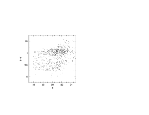
Fig. 8 shows a colour-magnitude diagram of the star sample, including three variable stars and the blue WDwarfs. We would like to point out again, that our WDwarf class contains indeed not only white dwarfs but all stars bluer than spectral type F. This includes BHB (Blue Horizontal Branch) stars, Blue Stragglers and sdB stars. The proper white dwarfs are actually only discovered if they are hotter than 6000 K, but we would expect no cool object in our small fields anyway.

6.2 Galaxies

A query for $MC\_class=^{\prime}Galaxy*^{\prime}$, $phot\_flag<8$ and $16<Ap\_Rmag<24$ selects 11343 objects from the catalogue. A sample of 86 further galaxies at $Ap\_Rmag<24$ have bad $phot\_flag\geq 8$. Constraining the sample with good flags ($<8$) to those with MEV redshifts yields 10046 objects. The remaining 1297 galaxies are virtually all fainter than $R=23$, reflecting just the incompleteness of MEV redshift estimation at faint magnitudes. Some 13000 fainter $R>24$ galaxies have redshifts, but they are of decreasing quality and certainly form in no sense a complete sample.

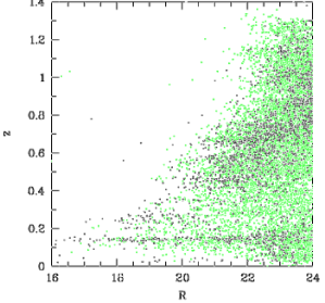
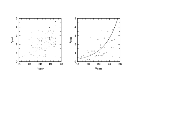
Fig. 8 shows a Hubble diagram of the galaxy sample revealing some structure in redshift space as well as a few maybe surprisingly bright objects. One of them is probably a misclassified star, the nature of the others is currently unclear. We suggest to exclude them from any sample for statistical studies.

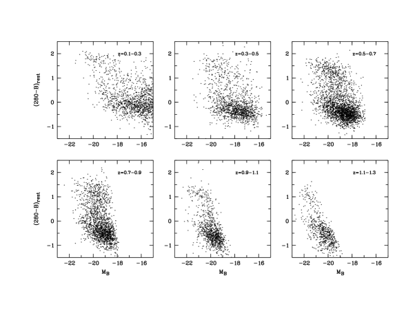
Fig. 9 shows colour-magnitude diagrams of the galaxy sample in several redshift slices. A clear bimodal distribution with a red-sequence and a star-fomring blue cloud can be seen at all redshifts.

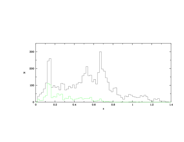
Fig. 10 shows the redshift distribution of galaxies with $R<21$ or with $R<23$. It deviates from the mean expected distribution due to the finite size of the field and large-scale structure. A cluster at $z\sim 0.15$ is clearly visible and the known sheets at $z\sim 0.67$ and $z\sim 0.73$ (Gilli et al., 2003) are blended into one peak in this histogram.

6.3 Quasars

A query for $MC\_class=^{\prime}QSO*^{\prime}$ and $16<Ap\_Rmag<24$ selects 97 objects. They all have MEV redshifts and no bad flags (see Fig. 11). Fainter QSOs could be selected, but probably with low completeness. We also inspected the subarea observed by the Chandra X-ray observatory for 1 Msec. Across all redshifts 16 type-1 AGN with $M_{B}<-21.7$ were identified by spectroscopic follow-up (Szokoly et al., 2004). A comparison reveals that COMBO-17 missed only one of the 16 type-1 AGN, suggesting a selection completeness of type-1 AGN well above 90% even into the Seyfert-1 luminosity regime (see Fig. 11).

The Deep Field observations of Chandra and XMM pick up almost all QSOs found by COMBO-17 in their fields of view. Only six out of 48 QSOs in the XMM area are not contained in the XMM source catalogue. Three of these are in the Chandra area and are confirmed as AGN with redshifts. A fourth one is a very weak, marginal Chandra source, and the remaining two are outside of the Chandra area. Hence, we don’t know whether Chandra would have detected them in 1 Msec observations.

6.4 Strange objects

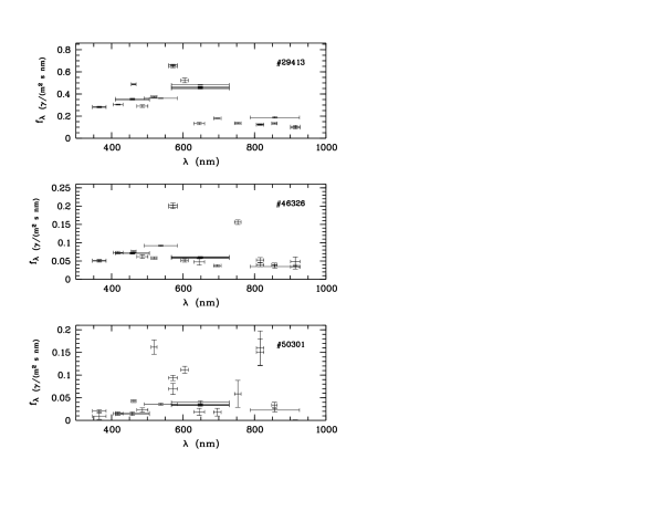
A query for $MC\_class=^{\prime}Strange\leavevmode\nobreak\ Object^{\prime}$ at $16<Ap\_Rmag<24$ selects three objects, none of which has bad flags (see Fig. 12). The first one of these, object 29413, is an isolated point source of $R\sim 21$. It shows no signs of variability, because the four $R$-band measurements from different epochs are totally consistent. But it appears quite hard to explain its SED without brightness variations. The $R$-band appears much brighter on the whole than some patches within its broad passband, which are probed by the medium-bands redwards of 600 nm. In a non-variable source this would imply enourmous fluxes between the low medium-bands. At this stage, we have no explanation for the nature of this object.

The second object (46326) is an extended source of $R\sim 23$ and can easily be explained by a galaxy with extremely strong emission lines. A plausible explanation places this object at $z\sim 0.15$, so it would show its H$\alpha$/Nii lines in the filter 753/18 and its H$\beta$/Oiii line in the filters 571/25 and $V$-band. The 753/18-filter shows emission at an equivalent width of $\sim 55$ nm within its limits of transmission, while 571/25 and $V$-band consistently show $\sim 50$ nm of emission.

The third object (50301) is totally swamped in the scattered light halo of a superbright ($R\sim 10$) foreground star. It is probably not safe to interpret the measured SED for this object.

6.5 Variable objects

COMBO-17 is not tailored to detect variability in any complete sense. Still, a query for $var\_flag>0$, $phot\_flag<8$ and $16<Ap\_Rmag<24$ selects 175 variable objects in the CDFS. Four more variables have bad flags. Three of them are stars, presumably two RR Lyrae and one M star (see Fig. 8). All others are classified as QSOs and galaxies.

At $R<22$, 34 out of a total of 39 QSOs are observed to be variable already in the COMBO photometry, while at $22<R<24$ the fraction is 32 out of 58 QSOs. Hence, the rate of observed variability drops from 87% to 55% due to the increased photometric noise that requires higher amplitudes to detect variability.

We note, that within the Chandra 1 Msec many of the variable galaxies are detected in X-rays and some of these have spectroscopic IDs as AGN. Some variable galaxies are likely to be rendered as such by Supernovae (see Wolf et al. 2001c for some cases).

Figure 13: Number counts: The black solid line shows all objects in the catalogue. The grey line shows the subset of classified stars in the left panel and the subset of galaxies with MEV redshift estimates in the right panel. The counts are plotted over the total magnitude $Rmag$.

Figure 14: Completeness map: Grey-scale maps of completeness from Monte-Carlo simulations of the survey (black: 100%, light grey 0%). Left panel: Stars, $B-V$ colour vs. $R$-band magnitude. Center panel: Galaxies, redshift vs. $R$-band magnitude. Right panel: Quasars, redshift vs. $R$-band magnitude.

7 Simulations of survey performance

7.1 Basic technique

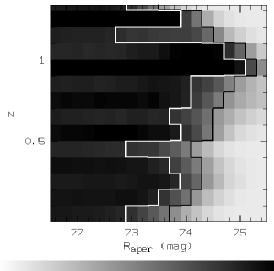
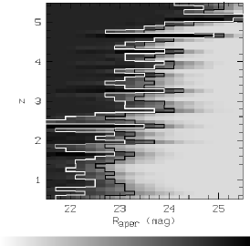
We carried out simulations of the survey in order to map completeness and contamination expected for the filter set and imaging depths given in COMBO-17. The basic technique was already described in WMR: We created lists of test objects from the colour libraries in Sect. 3 across a range of aperture magnitudes as in $Ap\_Rmag$. For each object in the library we determined filter fluxes and photometric errors. Then we scattered the flux values of the objects according to a normal distribution of the errors seen in the COMBO-17 observations. Finally, we recalculate the resulting colour indices and index errors and use this object list as an input to the classification.

The simulations show how well the classification can potentially work, assuming that library spectra precisely mimic real objects. In reality, differences between assumed and real SEDs will degrade the performance. Nevertheless, the simulation highlights the principal shortcomings of the method itself and the chosen filter set in particular.

We run these tests for stars, galaxies and quasars with magnitudes in the range of $R=[21.6,25.4]$, in order to see how the classification degrades from optimum to useless with decreasing object flux. At $R=23$ objects are measured roughly at photon noise levels of 10-$\sigma$ in the medium-band filters. But for bright objects, calibration errors and fine differences between real and model SEDs dominate the total errors. Thus, we first add a 5% uncertainty quadratically on top of the colour index errors before applying the classification, just as we do it with real catalogue objects. The performance of the classification converges to its best level at $R\la 22$. At the other end, $R\approx 25$ objects are well detected only in the broad-band filters, while the medium bands yield only fluxes with errors higher than 40%. We expect the survey to be almost useless at this level. We use one realisation of each library at each point in magnitude value. The latter are spaced in steps of $0\aas@@fstack{m}2$. This leads to a total of, e.g., about 1.3 million galaxies in the simulation.

Finally, we compare the classes and redshifts of the classified output with those defining the input objects. For any object type and redshift range, we can quantify the completeness of the classification as the fraction of input objects which are recovered correctly. But we can also look at the rate of objects being misclassified and hence contaminating samples of other classes. In the following, we discuss the completeness and contamination maps in detail.

7.2 Expected completeness of class samples

7.2.1 Stars

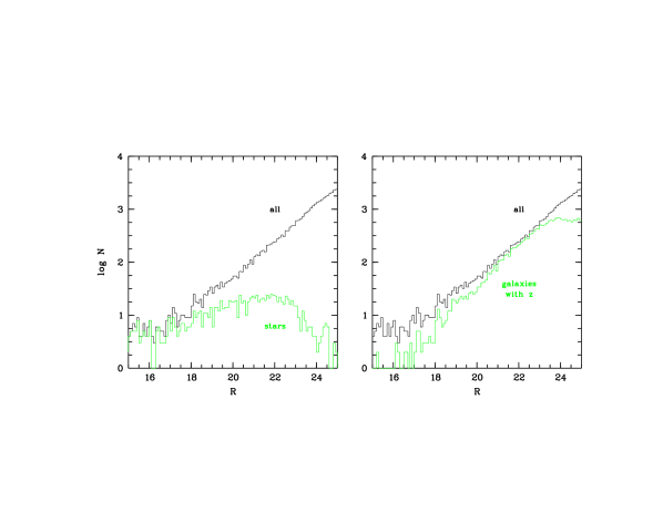
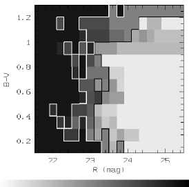
The completeness of star samples depends on their colour and magnitude as shown in the map of Fig. 14. The map suggests that for stars with $B-V<1.0$ (roughly spectral types FGK) the completeness does not vary much with colour, only with magnitude. The 90% completeness limit of FGK stars is at $R\approx 22.5$ and the 50% level is reached around $R\approx 23.2$. Redder M stars at $B-V>1.0$ appear much brighter in the far-red bands for any given $R$ magnitude. Also, they are among the reddest objects of all templates. Both factors help to increase the $R$-band depth of their successful classification. The result of these simulations is confirmed by the observed completeness limits in the stellar sample. The colour-magnitude diagram of the star sample in Fig. 8 shows how the M stars reach deeper than bluer stars. The average completeness can be better assessed from the number count plot of all objects vs. the stars in Fig. 13.

7.2.2 Galaxies

The completeness of galaxy samples not only depends on magnitude and redshift (see Fig. 14), but also on the restframe colours of the galaxy. This map, however, shows the average completeness for galaxies of all colours. The depth of the overall classification increases when going from $z=0$ to $z=1$ mostly because red galaxies can be identified to greater depth with increasing redshift, as they turn into increasingly red objects with increasingly bright far-red fluxes for given $R$-band magnitudes (like M stars). For the bluest starburst galaxies, the depth of the classification changes hardly with redshift. This is discussed in more detail in Wolf et al. (2003a), although actual map details have changed following the changeover in templates. Again, the completeness derived from number count plots (see Fig. 13) confirmes the basic result of the simulations.

7.2.3 Quasars

A previous version of the completeness map for quasars in COMBO-17 has already been published in a paper on the evolution of the luminosity function of quasars (Wolf et al.  2003b, ). However, the recent change in the galaxy templates has also affected the quasar classification, and here we present the updated map for the catalogue published here. The map shows oscillations in the depth of the classification. They are caused by the signature of strong emission lines migrating through the filter set and changing between strong visibility in a medium-band filter and invisibility in the spectral blind spots between the medium-band filters.

This completeness map assumes QSO spectra to comprise only AGN light, being based on the SDSS template and dominated by high-luminosity QSOs. Mixing stellar light into the SEDs should reduce the completeness until the AGN nature can not be detected any more. If host galaxies dominate the spectrum of an active galaxy, it will not be classified as a QSO but as a galaxy. Fig. 11 compares broad-line AGN identified in X-ray follow-up with QSOs identified by COMBO-17 in the same area. It suggests, COMBO-17 is $>90$% complete at picking out type-1 AGN with luminosities above $M_{B}=-21.7$, but starts to fail below that level of nuclear activity. A consistent explanation involving the simulated map and the nuclear contrast issue works as follows: at low redshifts the real limitation is the nuclear activity level depressing the observed completeness below the simulated one. At higher redshifts the limit of $M_{B}=-21.7$ drops to faint apparent magnitudes where the survey depth limits identification.

Figure 15: Contamination maps: Grey-scale maps of class cross-contamination from Monte-Carlo simulations of the survey (black: more contamination, light grey: no contamination, normalisation arbitrary, details see text). Left panel: Stars, misclassified as galaxies at redshift $z$ vs. $R$-band magnitude. This map basically reflects the incompleteness of the star selection at faint magnitudes. Center panel: Galaxies at redshift $z$ vs. $R$-band magnitude, which are misclassified as stars. Especially, around zero redshift, galaxy SEDs are easily confused with SEDs of stars. Right panel: Galaxies, misclassified as quasars at redshift $z$ vs. $R$-band magnitude.

7.3 Expected contamination in class samples

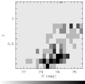
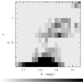
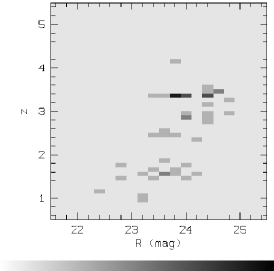
There is a multitude of contamination maps we could possibly wish to plot. Each of the four classes can lose objects to the other three classes. Each of those twelve plots can be shown over two sets of class parameters — if you wish to see where you lose objects from a class you plot the map over input parameters, and if you wish to see where exactly they go, you plot it over output parameters. Here, we just present the three most important contamination maps (see Fig. 15).

The biggest issue in the whole COMBO-17 classification is confusion between stars and galaxies. First, all stars not successfully identified as such are either classified as Galaxy or Galaxy (Uncl). The chances of a star being mistaken as a quasar are less than 1 in 1000 as far as the simulations are concerned (although stars outside our template range pose a problem, like binaries of M dwarf$+$white dwarf). So, the incompleteness of stars at $R>23$ translates directly into a contamination of the galaxy class there. At $R=23.5$, the map suggests that a quarter of all K stars are turned into Galaxy (not counting Galaxy (Uncl)), and at $R=24$ it is already two thirds.

How much trouble K stars mean for any analysis of galaxy samples depends on the number counts of stars, and hence on the Galactic coordinates. We briefly discuss a very rough estimate for the CDFS: We expect about 200 stars per magnitude bin at $R\sim 23$, of which (roughly guessing) 80 may be K stars. In the end, the contamination maps seem to suggest that at $R=[23,24]$ around 20 to 40 K stars are misclassified as Galaxy. In ground-based seeing, it will be hard to reliably identify the stars with a morphological criterion, because some faint galaxies will also be considered unresolved. A final classification could be settled using the HST imaging of GOODS and GEMS.

We note, that M stars ($B-V>1$) are correctly identified to fainter levels than K stars and do not pose a big problem. This is plausible given that they show more flux in far-red filters, securing their identification.

Second, even at brighter levels there is confusion between certain stars and galaxies near redshift zero due to their intrinsically similar colours. The maps indicate that almost 1% of the galaxies at $z<0.15$ and $R=[22,24]$ end up being classified as stars, if we do not override the statistical class decision by a morphological criterion. The catalogue contains about 750 galaxies within these limits, ten of which would have been classified as stars if it were not for the extended morphology (see Sect. 4.4 and 4.6).

A less important problem are galaxies contaminating the quasar class. In pure broad-band surveys this is an important issue, but in COMBO-17 it appears to be less relevant. The simulations suggest there would be a 1-in-10000 chance that galaxies at $R\sim 24$ are mistaken as quasars. This would imply one fake quasar at $R<24$ which is really a galaxy. But the main contamination in the quasar class probably arises from objects with unusual spectra not represented by the templates, hence there could be a few objects in total.

The last relevant issue is that of quasars contaminating the galaxy class. Here, again the completeness maps of quasars suggest that whatever quasar is not successfully identified, will end up in the galaxy sample. We have discussed above in detail, that proper quasars of $M_{B}<-23$ are probably all correctly identified, while incompleteness in the detection of fainter type-1 AGN is mostly a matter of their activity level and the contrast of their nuclear light to their host galaxy.

Figure 16: Redshift quality expected from Monte-Carlo simulations: Galaxies at $z=0.1\ldots 1.1$ (top row, solid line: early types, dashed line: late types) and QSOs at $z=1\ldots 4$ (bottom row). Left panels: Completeness of classification combined with redshift determination, for redshift values of the Minimum Error Variance (MEV, black line) and the Maximum Likelihood (ML, grey line) method. Center panels: 1$\sigma$-scatter in true redshift error. Right panels: mean offset in estimated $z$ from simulated $z$. The QSOs appear to have extremely high redshift accuracy still at faintest levels, but only because the completeness drops drastically and is reduced to the most conspicuous QSOs.

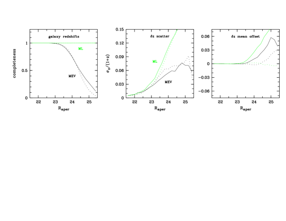
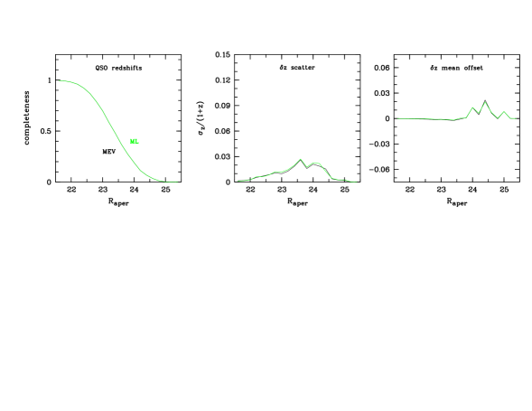
7.4 Expected redshift errors

From the simulations we can estimate expected redshift errors by comparing the input redshifts with recovered estimates. If objects are bright enough, redshifts are measured equally well for galaxies and QSOs, both of which have enough spectral features. If objects are faint, weak spectral features are washed out more effectively by noise than strong features, and it is not a-priori clear how the redshifts of different objects are affected.

When changing redshift, the fixed wavelength resolution of the filter set translates into an error that scales with $(1+z)$. Therefore, we shall discuss redshift errors only in terms of $\delta_{z}/(1+z)$ to remove this obvious dependency.

When changing magnitude, we implicitly change the average redshifts and spectral types of a sample. Having eliminated the influence of redshift above, we can split the sample into different spectral types and look only at the influence of magnitude. Essentially, a magnitude change is a change in S/N ratio across all filter fluxes and hence on the measured SED. To first order, redshift errors should be proportional to the radii of error ellipsoids in colour space, provided the mapping from redshift to colour space is not too non-linear. Because photometric errors increase inversely proportional to a decreasing flux, we expect mean redshift errors to scale as $\sigma_{z}/(1+z)\propto 1/F$ with $F$ being the mean flux of an object.

However, Poisson noise is not the only source of photometric error because the relative calibration of the passbands is also subject to uncertainties as well as variations in real object spectra which are not reflected in the sequence of templates. These additional effects cause mismatches between object and templates which are non-Gaussian in shape and non-Poissonian in magnitude dependence. They are actually independent of magnitude, although the mean template mismatches could change due to a change in the underlying sample. When going fainter, the calibration error should matter less and less in comparison to the Poisson error. But the faint object population is less well known and might harbour surprising challenges for the templates.

Furthermore, most known objects cover only a finite volume in colour space, and hence require a finite error to be discriminated. At some low signal level, the classification will just break down, because there are plenty of interpretations possible for the noisy observed SED. Here, some a-priori knowledge from the literature could guide an interpretation if needed.

We like to repeat here our division of the magnitude scale with respect to the quality of classification and redshifts into three basic domains:

1. the quality saturation domain at $R<22$ limited by systematic errors

2. the quality transition domain at $R=22\ldots 24.5$ limited by photon noise

3. the quality breakdown domain at $R>24.5$ which is useful only in conjunction with (and limited by) a-priori knowledge.

7.4.1 Galaxies

We average the simulated redshift accuracy across a range in redshifts chosen to match the bulk of the observed population, thus running from $z=0.1$ to $z=1.1$. We split the full galaxy sample into red-sequence galaxies and star-forming blue-cloud galaxies to check for differences in accuracy. In each magnitude bin, we determined the mean offset among the redshift deviations $\delta_{z}/(1+z)$ to check for a possible bias, and calculated the scatter. Between the two galaxy types we found little difference (see Fig. 16). We also compared the redshifts from a Maximum-Likelihood (ML) estimator with the Minimum-Error-Variance (MEV) estimator that we use routinely. As explained above, we ignore the MEV measurement when its error goes above a threshold (see Sect. 4.5). We found the scatter of MEV redshift deviations to be below the scatter of ML redshifts. At bright magnitudes, where both redshift exist for all objects, this shows the superior performance of the MEV estimator (which is by design). At faint magnitudes, only those objects have MEV redshifts which have not too wide $p(z)$ distributions and are not expected to have strong deviations in the first place. This selection keeps the scatter of MEV redshift deviations much below the ML curve.

The simulations suggest that MEV redshifts should be roughly wrong by $\sigma_{z}/(1+z)\la 0.01$ at $R<22$, and throughout the quality saturation domain. Towards $R=24$ the mean redshift scatter should increase to 0.06 whereas the fraction of galaxies with MEV estimates has dropped to $\sim 75$%. In the quality breakdown domain, the scatter does not increase by much, but the fraction of objects with MEV estimates is extremely small.

Figure 17: Redshift quality of galaxies: Top row: 404 bright galaxies observed with 2dF, mostly containing galaxies from the supercluster field A901/902. Left panel: Redshift comparison $z_{phot}$ vs. $z_{spec}$. Center panel: Redshift error $\delta z/(1+z)$ vs. redshift $z_{spec}$. Right panel: Redshift error $\delta z/(1+z)$ vs. aperture $R$-band magnitude. The 1-sigma redshift error is $<0.01$, and the outlier rate for errors above 0.05 is $<$1% (3 out of 404 objects with errors around 0.06). Center row: A sample of 162 faint galaxies. Objects fainter than $R=23.5$ are shown in grey. Objects with redshift deviations above 0.15 are shown as arrows. Bottom row: 247 galaxies from the K20 survey by Cimatti et al. Arrows in center or right column panels represent outliers with more than 15% redshift error in (1+z).

Figure 18: Redshift quality of AGN: Panels are as in Fig. 17. The active galaxy sample is from the Szokoly et al. (2004) follow-up of X-ray sources, and contains 24 Sy-1 and 41 Sy-2 objects, cut off here at $R<24$. Their QSO sample contains 20 QSO which we have supplemented with seven QSOs from 2QZ on the S11 field and a QSO from slitless spectroscopy in the CDFS. The average redshift error of QSOs is $\approx 0.015$ with two outliers in 27 objects.

Figure 19: Summary of galaxy redshift quality: This figure contains all 813 galaxies from all available samples. Individual redshift deviations have been averaged within full magnitude bins, and the resulting zeropoint offsets and the 1-$\sigma$ scatters are shown as black error bars. Furthermore, the 1-$\sigma$ redshift errors predicted by the simulations are plotted as solid lines at $R>21.6$.

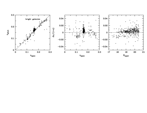
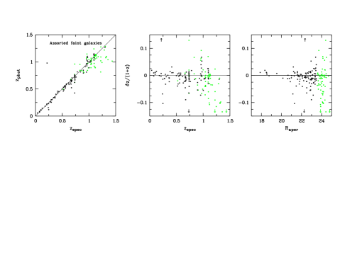
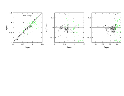
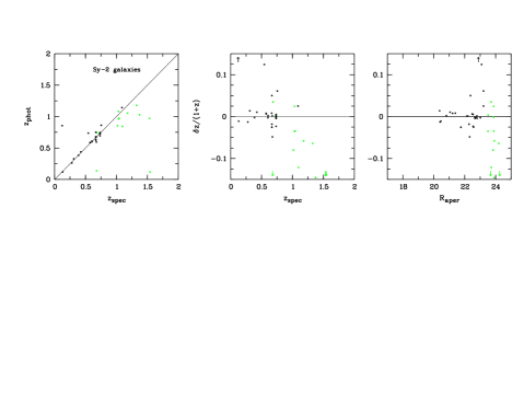
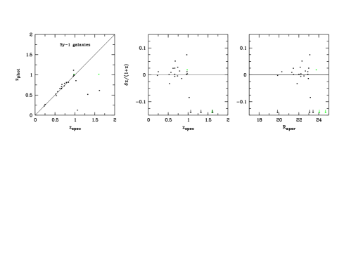
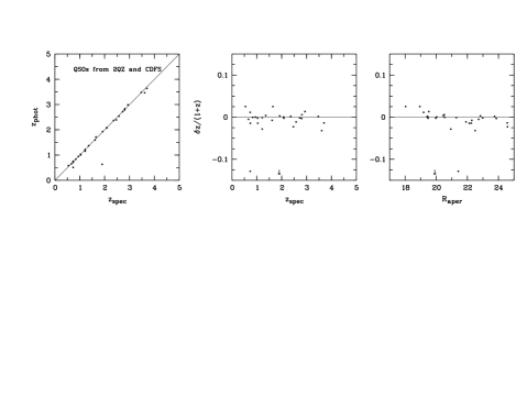
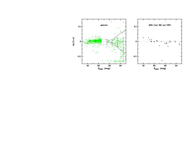
7.4.2 Quasars

We also determined the mean offset and scatter for quasar redshifts, across the redshift range of the bulk sample, from $z=1$ to $z=4$. The results for the ML and MEV estimator are virtually identical. Even the completeness of the ML estimator drops with magnitude, because not all quasars are identified as such. At faint levels, many simulated quasars are mistakenly identified as galaxies and have wrong redshifts assigned. In Fig. 16 we only look at redshift deviations of recognized quasars because only those would be in an observed quasar sample. We found the scatter and offset to be generally very low at all magnitudes. This is because, whenever a quasar is recognized as such, its spectral features were strong enough to get its redshift right, with an average error of $\sigma_{z}/(1+z)\la 0.015$.

8 Spectroscopic performance test

Currently, we have several independent spectroscopic samples available to test the quality of classification and redshifts in COMBO-17: there are complete samples from 2dF spectroscopy on three COMBO-17 fields, X-ray follow-up in the CDFS (Szokoly et al. 2004), and the K20 survey (Cimatti et al. 2002)in the CDFS. The 2QZ survey overlapping with the S11 field is basically complete, but does not cover QSOs at all redshifts. An important but incomplete sample is the VLT/FORS spectroscopy on the CDFS started by GOODS. Altogether, these samples comprise spectra of 37 stars, 813 inactive galaxies, 28 QSOs and 65 active galaxies. Almost all these objects are brighter than $R=24.5$.

8.1 Stars

The spectroscopic samples contain 37 stars. Four of these were observed in Chandra follow-up and 33 mostly red stars were contained in the K20 survey. The faintest one ($R=23.3$) out of the 37 was wrongly classified by us as a galaxy, while the other 36 were correctly identified as stars. We believe, that at $R\ga 23$ there could be problems with mixing up red stars and red-sequence galaxies. But at $R\la 23$ these findings suggest that the stellar sample is complete.

8.2 Galaxies

8.2.1 Bright galaxies observed with 2dF

Spectroscopy of bright galaxies was available through the 2dFGRS survey on the S11 field with 39 galaxies including the cluster A1364 at $z\sim 0.11$ and 14 galaxies on the CDFS field, most at $R\la 18$. Proprietary observations on the A901 field provided a larger and deeper sample of 351 galaxies at $R\la 20$ including the cluster A901/902 at $z\sim 0.16$. The total number of independent redshifts is 404. We will assume here that the classification quality is the same across all COMBO-17 fields. Fig. 17, top row, displays the redshift quality of these bright galaxies. We find that 77% of all galaxies have redshift errors $\delta_{z}/(1+z)$ below 0.01 and three objects, i.e. less than 1%, deviate by more than 5-$\sigma$ from the true redshift.

8.2.2 Assorted faint galaxy samples

In the faint domain we have no very large and complete spectroscopic sample available. Hence, we have opted for collecting assorted samples from various authors as far as possible. Here, we include 31 inactive galaxies observed by Szokoly et al. (2004), 21 red-sequence galaxies around $z\sim 1$ observed by Franx et al. (2004), and 110 galaxies observed with FORS2 by GOODS. The GOODS sample is larger than this, but we excluded repeat measurements with the other sources after confirming their consistency. At this stage, we restricted the sample to objects with secure line identification (Kuntschner, priv. comm.). More objects might become available soon. The top row of Fig. 17 shows the redshift quality of this assorted sample.

Figure 20: Galaxy redshift errors: true deviations divided by estimated errors vs. estimated errors. In a truely Gaussian scatter we expect $\sim 68$% of a sample to fall into $[-1,+1]$. In our sample this is in fact the average behaviour although there is a non-Gaussian tail to larger-than-expected deviations.

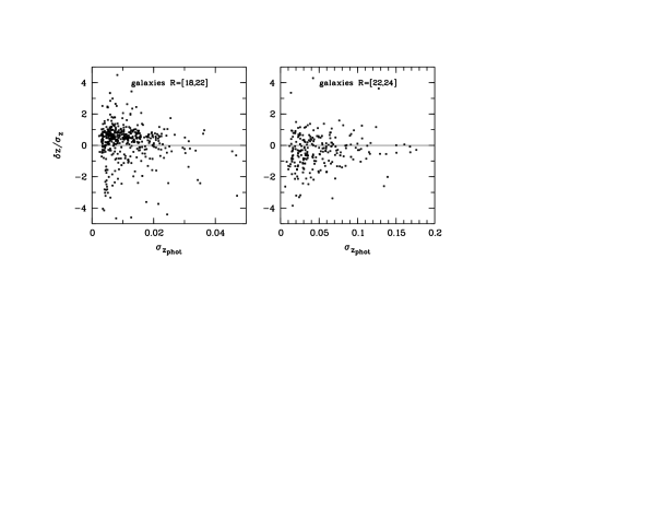
8.2.3 K20 sample

We present the redshift comparison with the K20 sample (Cimatti et al. 2002) separately, because it is a complete sample, at least in terms of $K$-band selection, although not in terms of an $R<24$ selection. It preferentially contains red objects, while faint blue galaxies would be underrepresented. Excluding stars and broad-line AGN we selected 247 objects with $K_{s}<20$ and their spectroscopic quality equal to 1, signifying reliable redshift. The COMBO-17 redshift quality from this comparison is shown in the bottom row of Fig. 17. We see the same result as for the assorted sample above except for a somewhat higher outlier rate.

8.2.4 Galaxy summary

At $R\la 24$ and $z\la 1$ we seem to have (1-$\sigma$) redshift errors that could be described analytically by

$$\sigma_{z}/(1+z)\approx 0.007\times\sqrt{1+10^{0.8(R-21.6)}}\leavevmode\nobreak\ .$$ (5)

The rate of outliers appears to be below 5% at $z\la 1$. We would like to note, that even spectroscopic redshift determination can be challenging if only one line is clearly visible. In such cases, the overall SED shape from COMBO-17 or its own redshift estimate can be helpful to spectroscopic work in order to reach a final interpretation of an observed line. Finally, any blended objects will completely fool the COMBO-17 approach which probably can not decompose a spectrum into two. Spectroscopy of sufficient quality and spatial resolution can deal with those rare challenges much better.

In Fig. 20 we compare the true redshift deviations with individual 1-$\sigma$ redshift uncertainties estimated by the template matching code. As expected we find a scattered distribution of true deviations around the expected mean. We find, that objects with larger estimated errors have true deviations as expected from the mean or slightly below. In contrast, objects with extremely small estimated errors scatter a bit more than expected from the error estimation. A Gaussian distribution puts $\sim$68% of a sample below its 1-$\sigma$ cut. We find numbers between 53% and 78% in different subsamples of our galaxies. Bright, large-error galaxies ($R=[18,22]$ and $\sigma_{z}>0.01$) have more accurate redshifts than expected: 78% are at $\delta z<\sigma_{z}$. Faint, small-error galaxies ($R=[22,24]$ and $\sigma_{z}<0.03$) have less accurate redshifts than expected: 53% are at $\delta z<\sigma_{z}$. Bright, small-error objects and faint, large-errors objects behave as expected with $\sim 70$% at $\delta z<\sigma_{z}$.

Table 6: COMBO-17 classification and 2dF spectroscopy of QSO candidates from the 2QZ survey on the S11 field. Note, that COMBO-17 detected all true quasars at the right redshift, and that it was able to discard all false candidates except for a white-dwarf/M-dwarf binary, for which no matching templates existed.

COMBO-17				2QZ
Identifier	$R$ (mag)	class	$z_{phot}$	$z_{2dF}$	class
S11-03978	19.47	QSO	2.078	2.086	QSO
S11-17931	17.99	Star			cont
S11-18345	20.00	QSO	2.078	2.077	QSO
S11-19860	19.55	Galaxy	0.134		??
S11-22644	18.89	WDwarf			star
S11-36451	19.53	QSO	2.987	2.935	QSO
S11-36868	19.57	QSO	0.596		WD(DA)
S11-40157	20.45	QSO	1.367	1.358	QSO
S11-40953	19.44	QSO	0.944	0.944	QSO
S11-42872	18.01	QSO	1.714	1.647	QSO
S11-43560	19.43	QSO	2.367	2.360	QSO
S11-45585	20.07	Star			star
S11-48688	20.09	Star			??
S11-52614	20.51	WDwarf			??

8.3 AGN sample in CDFS and S11 field

The spectroscopic follow-up of X-ray sources in the CDFS Szokoly et al. (2004) provides a very good sample to test the completeness of AGN detection in COMBO-17 (see Fig. 18). As already discussed above, the QSO class is a complete sample of type-1 AGN at $M_{B}<-21.7$ and contains an incomplete set of low-luminosity type-1 AGN. Whenever the host galaxy dominates the SED and nuclear light from a low-luminosity AGN is only a fraction of that, COMBO-17 considers the object as a Galaxy and basically determines the redshift of the host galaxy. From COMBO-17 alone, we have no means to identify the nuclear activity in AGN of such low luminosity. The same applies to type-2 AGN, where again the host galaxy dominates the visual SED by far.

Another question is whether the host galaxy redshifts of low-luminosity AGN are estimated correctly, or whether the presence of the AGN light leads to problems. Hence, we investigate the redshift quality of that fraction of the COMBO-17 galaxy sample, which has been classified as Sy-1 or Sy-2 by Szokoly et al. (2004) on the basis of X-ray data and optical spectroscopy.

We find that for objects at $z\la 1$ the redshift estimation behaves like it does for normal galaxies with the exception of a remarkably faint dwarf Sy-2 object (see also Sect. 4.6). This object has $R_{total}=22.6$ and shows an SED that perfectly matches a red-sequence galaxy at $z\approx 0.85$. But the spectroscopy shows emission lines at $z=0.122$ on top of a remarkably red continuum. If all the light originated in fact from a source at $z=0.122$, this galaxy would be a dwarf Sy-2 with a total luminosity of $M_{B}\approx-14.5$ and a truely unusual continuum. If the object was a blend of two and most of the light came from a background galaxy, the host of this AGN would be even fainter.

At $z>1$ we find that Sy-2 galaxies behave still much the same as normal galaxies, but Sy-1 galaxies produce three outliers. Here we are probably confronted with restframe UV SEDs which are a mix of host galaxy light and nuclear light confusing the classification. The Sy-1 galaxies are the weakest feature of classifier. Presently it is not clear, whether sufficient templates could be defined which could alleviate this problem.

Finally, the redshifts of QSOs (including seven objects from 2QZ and one object from slitless spectroscopy on the CDFS) have errors of $\sigma_{z}/(1+z)\approx 0.015$, independent of magnitude. This is plausible because QSOs have sufficiently strong spectral features to pin down their redshifts, except for a low-redshift outlier, which is off by 0.13, and a $z\sim 2$ outlier whose redshift is completely wrong. Providing identifications and photometric redshifts for quasars at 1.5% accuracy is one of the strongest advantages of COMBO-17.

We would like to report also on spectroscopic cross check available from the 2dF Quasar Redshift Survey (hereafter 2QZ, see Tab. 6) on the S11 field of COMBO-17. The seven QSOs identified there by 2QZ have already been included into Fig. 18. But in addition, we present the full table of 2QZ candidates and their spectroscopic ID as obtained with 2dF in Tab. 6. We compare the spectroscopic result with our classification and demonstrate that COMBO-17 provides almost equivalent information, with two restrictions: (i) COMBO-17 misinterpreted an M-dwarf/white-dwarf binary as a quasar; (ii) The COMBO-17 redshifts are obviously less accurate at a level of $\sigma_{v}\la 5000$ km/sec.

9 Summary

Wolf, Meisenheimer & Röser (2001) showed that medium-band surveys deliver more accurate object classifications and photometric redshifts than broad-band surveys, while not consuming more telescope time. As a result, the COMBO-17 survey was started to obtain a large redshift catalogue of galaxies and AGN for evolutionary population studies, including weak lensing observations.

In this paper, we have discussed in detail the quality of the classification and photometric redshifts of galaxies and quasars in COMBO-17. We have shown that the identification of stars is complete to $R\la 23$ (deeper for M stars). We have demonstrated that the identification of type-1 AGN is complete above luminosities of $M_{B}=-21.7$ at all redshifts from 0.5 to 5. The photometric redshifts of galaxies in COMBO-17 are better than 0.01 at bright magnitudes ($R<21$) and increase with photometric noise to $\delta_{z}/(1+z)\approx 0.06$ at $R=24$. Fainter than $R=24$, COMBO-17 is not particularly useful because the medium-bands are too shallow then. We have demonstrated that we routinely obtain photometric redshifts of quasars and luminous Seyfert-1 galaxies to an accuracy of $\delta_{z}/(1+z)\approx 0.015$.

We have demonstrated that the medium-band approach indeed delivers the expected performance which motivated the survey COMBO-17. In this paper we now deliver the COMBO-17 database from one particular patch of sky to the community for public exploitation. The published database includes images and a catalogue with 63,501 objects. Classification and redshifts are typically reliable at $R<24$, where we find $\sim 100$ quasars, $\sim 1000$ stars and $\sim 10000$ galaxies.

We included the Chandra Deep Field South from the very beginning in the COMBO-17 project. A multitude of deep observations was expected across a wide range of photon energies, creating a unique data set for studies of galaxy evolution. The COMBO-17 approach has allowed us to get hold of a large redshift catalogue on the field. This includes the implicit selection of $\sim 100$ luminous type-1 AGN with photometric redshifts as accurate as $\sim 5000$ km/sec. We are now in a position to make this catalogue available for general use and hope to feed many more dedicated follow-up studies.