uvby-$\beta$ photometry of high-velocity and metal-poor stars

$uvby$(–$\beta$) photometry has been obtained for an additional 411 very metal-poor stars selected from the HK survey, and used to derive basic parameters such as interstellar reddenings, metallicities, photometric classifications, distances, and relative ages. Interstellar reddenings adopted from the Schlegel et al. (1998) maps agree well with those from the intrinsic-color calibration of Schuster & Nissen (1989). [Fe/H] values are obtained from the CaII K line index of the HK survey combined with the $uvby$ and $UBV$ photometry. The $c_{\rm 0},(b-y)_{\rm 0}$ diagram is seen to be very useful for classifying these very metal-poor field stars into categories similar to those derived from globular cluster color-magnitude diagrams; it is found that the HK survey has detected metal-poor candidates extending from the red-giant to the blue-horizontal branch, and from the horizontal branch to subluminous stars. Distances derived from $UBV$ photometry agree reasonably well with those from $uvby$, considering the paucity of good calibrating stars and the extrapolations required for the most metal-poor stars. These very metal-poor stars are compared to M92 in the $c_{\rm 0},(b-y)_{\rm 0}$ diagram, and evidence is seen for field stars 1–3 Gyrs younger than this globular cluster; uncertainties in the [Fe/H] scale for M92 would only tend to increase this age difference, and significant reddening uncertainties for M92 are unlikely but might decrease this difference. The significance of these younger very metal-poor stars is discussed in the context of Galactic evolution, mentioning such possibilities as hierarchical star-formation/mass-infall of very metal-poor material and/or accretion events whereby this material has been acquired from other (dwarf) galaxies with different formation and chemical-enrichment histories.

1 Introduction

Over the past two decades, our collective knowledge of the nature of the thick disk and halo of the Galaxy has expanded enormously, due primarily to the impact of several ongoing large-scale survey efforts carried out to detect and analyze metal-poor stars. These include the HK survey of Beers and collaborators (Beers, Preston, & Shectman 1992; Beers 1999) and the Hamburg/ESO stellar survey of Christlieb & collaborators (Christlieb 2003), both of which select stars with objective-prism techniques, and hence introduce no kinematic bias into their samples. Such biases are present (and must be corrected for) in proper-motion selected survey samples, such as the exhaustive previous studies of, e.g., Ryan & Norris (1991) and Carney et al. (1996). The prism-survey selected samples are hence well suited for studies of the kinematics and dynamics of the old stellar populations of the Milky Way, in particular because of the burgeoning databases of proper motion information that are presently being assembled from a variety of sources (e.g., UCAC2: Zacharias 2002; SPM: Girard et al. 2003). In order to make optimal use of the proper motions for kinematic analyses, accurate stellar classifications, and photometrically determined distances, are crucial.

The $uvby$–$\beta$ photometric system is particularly suited for the study of very-metal-poor (hereafter, VMP) F- and G-type stars, as has already been pointed out in Paper VIII by Schuster et al. (1996; hereafter S96). Briefly, intrinsic-color calibrations, $(b-y)_{\rm 0}$–$\beta$, exist which allow accurate and precise, $\pm 0\aas@@fstack{m}01$, measures of interstellar reddening excesses, $E(b-y)$, for individual field stars; such a calibration has been given by Schuster & Nissen (1989). Photometric absolute magnitudes and distances can be calibrated and used effectively, as shown in the papers by Olsen (1984) and Nissen & Schuster (1991). This photometric system has the great advantage that it permits us to obtain accurate stellar distances even for evolving main-sequence and subgiant stars due to the gravity sensitivity of the $c_{\rm 0}$ index. Also, importantly, theoretical isochrones in the $M_{\rm bol}$, $T_{\rm eff}$ diagram can be transformed to the $M_{\rm V}$, $(b-y)_{\rm 0}$ or $c_{\rm 0}$, $(b-y)_{\rm 0}$ diagrams for the estimation of relative and/or absolute ages of evolving field stars which are near their respective turn-offs, and in several of the previous papers of this series the isochrones of VandenBerg et al. have been used for such purposes, to study the Galactic halo population and to make comparative analyses between the relative ages of the halo and thick-disk stellar populations. Most recently the isochrones of Bergbusch & VandenBerg (2001) have been transformed to the $uvby$ photometric system using the color–$T_{\rm eff}$ relations of Clem et al. (2003).

Also, the $uvby$–$\beta$ photometry can provide basic stellar atmospheric parameters as a prelude to detailed chemical abundance studies making use of high-resolution spectroscopy and model atmospheres. Several empirical calibrations already exist in the literature for the conversion of $(b-y)_{\rm 0}$ or H$\beta$ to $T_{\rm eff}$; these calibrations include appropriate metallicity dependences. Index diagrams, such as $c_{\rm 0}$, $(b-y)_{\rm 0}$, or the reddening-free $[c_{\rm 1}]$, $[m_{\rm 1}]$, or $[c_{\rm 1}]$, $\beta$, allow the classification of field stars according to their evolutionary status, permiting us to estimate the stellar surface gravities, also for input into the model-atmosphere analyses.

In this paper, $uvby$–$\beta$ photometry is presented for an additional 411 VMP stars from the HK survey, providing a total database of such photometry for 497 VMP stars, when combined with the data of S96. For the present sample the stars have been selected with [Fe/H] $\la-1.5$, and 243 were observed in México using classical photometric (photoelectric) techniques and 177 in Chile using DFOSC (CCD) techniques. In Sect. 2 the observing and reduction techniques are described briefly, the catalogues of new $uvby$–$\beta$ data presented, and the $V$ magnitudes and $(b-y)$ colors from the $uvby$ observations compared to magnitudes and $(B-V)$ from the HK survey. In Sect. 3, the photometry is dereddened using a modification of the Schlegel et al. (1998) reddening maps and also the intrinsic-color calibration of Schuster & Nissen (1989); reddenings from the two methods, $E(B-V)$ and $E(b-y)$, are compared. In Sect. 4, [Fe/H] values are derived for the VMP stars using the techniques developed in the HK survey, and probable carbon-enhanced stars are identified based on a comparison of the GP and KP indices. Photometric classifications are derived for the VMP stars in Sect. 5 using the $c_{\rm 0}$, $(b-y)_{\rm 0}$ diagram. Stars are found covering a wide range of stellar types from the horizontal branch (HB) to subluminous stars (SL), and from the red giant stars (RG) to the blue horizontal branch (BHB), and other categories include main-sequence (MS), turn-off (TO), subgiant (SG), blue-straggler (BS), and red-horizontal-branch-asymptotic-giant-branch (RHB-AGB) stars. Possible abundance anomalies for some VMP stars have been identified from the $uvby$ photometric indices and diagrams, such as the $[c_{\rm 1}]$, $[m_{\rm 1}]$; for example, ten probable Am stars have been found and also a number of possible AGB stars with unusual chemical abundance ratios or binary companions. Distance estimates are made for the VMP stars in Sect. 6 using $uvby$ photometry plus various methods and new calibrations, and also using the $UBV$ photometry and techniques developed in the HK survey. Comparisons of these photometric distances show reasonably good agreement, considering the paucity of calibrating stars and extrapolations required for the more VMP stars. In Sect. 7, the VMP field stars are compared to the globular cluster M92 in the $c_{\rm 0}$, $(b-y)_{\rm 0}$ diagram, using the isochrones of Bergbusch & VandenBerg (2001), as transformed to $uvby$ by Clem et al. (2003), to interpolate relative and absolute ages. A number of VMP stars apparently 1–3 Gyrs younger than M92 are noted, and their importance for understanding the formation and evolution of the Galactic halo discussed.

2 Photometric observations of the very metal-poor stars

2.1 Selection of the stars

The VMP stars described herein were selected from two primary sources. The first set of 194 stars is a subset of the published catalogues of Beers, Preston, & Shectman (1985; BPSI) and Beers, Preston, & Shectman (1992; BPSII), using the criterion [Fe/H]${}_{c}\leq-1.5$, where [Fe/H]_c is the corrected spectroscopic metallicity estimate derived by BPSII based on a calibration of the strength of the CaII K index KP as a function of measured or inferred $(B-V)_{0}$ color. This set includes, primarily, stars at or near the main-sequence turnoff and warmer subgiants. The second set of 303 stars were candidate VMP stars selected from visual inspection of medium-resolution spectroscopy obtained during the course of the HK survey follow-up at a number of observatories, and includes stars covering a larger range of effective temperatures and luminosities. Since this second subset was selected prior to obtaining estimates of metallicity, it includes a larger fraction of stars exceeding [Fe/H] $=-1.5$ than the BPSI and BPSII subsample. The full set of HK-survey medium-resolution spectroscopic results will appear in a series of papers in preparation.

2.2 Observation and reduction techniques

The $uvby$–$\beta$ data presented here for the VMP stars were taken using $1.5\,$m telescopes and two different types of instrumentation. The data of Table 1 were taken during ten observing runs from September 1995 through November 2000 at the H.L. Johnson $1.5\,$m telescope at the San Pedro Mártir Observatory, Baja California, México (hereafter SPM), and the $uvby$ data of Table 2 during three runs from October 1998 through September 2000 at the Danish $1.5\,$m at the European Southern Observatory, La Silla, Chile (hereafter La Silla). For the SPM observing a six-channel $uvby$–$\beta$ photoelectric photometer was used, the same as for the Schuster & Nissen (1988; hereafter SN) and Schuster et al. (1993; hereafter SPC) catalogues and for the $uvby$–$\beta$ data of VMP stars by S96. For the La Silla observing the DFOSC has been used with a CCD detector, as described by Brewer & Storm (1999).

The $uvby$–$\beta$ data presented here for the VMP stars in Table 1 were taken and reduced using techniques very nearly the same as for SN, SPC, and S96. One is referred to these previous papers for more details; what follows is a brief outline of the more important points of the observational techniques. The four-channel $uvby$ section of the SPM photometer is really a spectrograph-photometer which employs exit slots and optical interference filters to define the bandpasses. The grating angle of this spectrograph-photometer was adjusted at the beginning of each observing run to position the spectra on the exit slots to within about $\pm 1{\AA}$. Whenever possible, extinction-star observations were made nightly over an air-mass interval of at least 0.8 (see Schuster & Parrao 2001), and spaced throughout each night several “drift” stars were observed symmetrically with respect to the local meridian, and with these observations the atmospheric extinction coefficients and time dependences of the night corrections could be obtained for each of the nights of observation (see Grønbech et al. 1976). Finding charts were employed at the SPM and La Silla telescopes to identify all of the stars from the HK survey. For previous studies, such as S96, the program stars were observed at SPM to at least 50,000 counts in all four channels of $uvby$ and to at least 30,000 counts for the two channels of H$\beta$; here, the fainter program stars at SPM ($V\ga 14\aas@@fstack{m}5$) were exposed to only at least $\approx 30,000$ counts in all four channels of $uvby$, and H$\beta$ was observed only for the brighter program stars ($V\la 14\aas@@fstack{m}0$) and to only $\approx 20,000$ counts in both channels at $V\approx 14\aas@@fstack{m}0$. For all program stars the sky was measured until its contributing error was equal to or less than the error of the stellar count. At SPM an attempt was made to obtain three or more independent $uvby$ observations for each of the program stars.

The $uvby$ observations for the VMP stars of Table 2 were taken using the C1W7 CCD (LORAL/LESSER backside illuminated chip) with 15 micron pixels, and a ESO $uvby$ filter set (Nos. 715, 716, 717, and 718). A more or less clean and uniform part of the chip was selected for the observations, and the Midas routine “point” was used to position the stars near the center of this area; for most nights the RMS positioning error was better than $\pm 2$ pixels, except for the more windy nights when it was $\ga\pm 2$ pixels. Since single stars were being observed, an area of only $250\times 250$ pixels was read out around the center of this “point” routine. In this way the observations could be read out rapidly and the filters cycled more quickly: $ybvu$ or $ybvuuvby$, with a bias taken after each cycle. Also, by reading $250\times 250$ pixels, four or more sky flats could be obtained in each filter-band during both the evening and morning twilights. By always centering the stars very nearly at the same place on the CCD, we could avoid major cosmetic defects, and also several problems of flat fielding, such as variations in the dispersed light. Whenever possible, atmospheric extinction observations were made nightly over an air-mass interval of at least 0.8. Extra biases were measured at the beginning and (sometimes) end of the nights, and a few 800s (or longer) dark measures were made during the observing runs (800s being the longest stellar integration). In general we attempted to obtain at least 22,000 ADUs in all bands for the program stars, corresponding to about 30,000e^-, and to obtain at least two independent observations for the program stars; this latter criterion was not accomplished for 86 of the La Silla program stars due mainly to poor photometric conditions during the last observing run.

For the CCD data from La Silla the IRAF package was used for the image reduction. All the images were bias, dark, and flat-field corrected employing the usual routines. The program and standard stars of this study were identified in all the fields and their centroids calculated. For each observed night, the FWHMs of all objects were averaged and from this average three different apertures from 3 to 6 times the $<$FWHM$>$ were tested. The PHOT routine was then used for extracting the instrumental magnitudes of all objects in the different filters. These instrumental values were then fed into the reduction programs of T. Andersen, described below, and reduced in the usual fashion. That extraction aperture which gave the smallest instrumental and transformation errors was then retained for the reduction of the final program-star standard photometry.

As for the SN, SPC, and S96 catalogues, all of these data reductions were carried out following the precepts of Grønbech et al. (1976) using computer programs kindly loaned by T. Andersen. At SPM the $uvby$–$\beta$ standard stars observed were taken from the same lists as for the previous catalogues; these are mostly secondary standards from the catalogues of Olsen (1983,1984). A few of the more metal-poor stars from Olsen and from the SN catalogue (such as HD2796, HD84937, HD140283, HD195363, BD$-17$:0267, and CD$-24$:1782) were observed often to be used as standard stars and to check for consistency. At La Silla the standard-star list was derived from stars with $V\la 10\aas@@fstack{m}5$ from SN, from S96, and from a 1998 version of our Table 1. The reduction programs create a single instrumental photometric system for each observing run, including nightly atmospheric extinctions and night corrections with linear time dependences. Then transformation equations from the instrumental to the standard systems of $V$, $(b$–$y)$, $m_{\rm 1}$, $c_{\rm 1}$, and $\beta$ are obtained using all standard stars observed during that observing period. The equations for the transformation to the standard $uvby$–$\beta$ system are the linear ones of Crawford & Barnes (1970) and of Crawford & Mander (1966). Small linear terms in $(b-y)$ are included in the standard transformation equations for $m_{\rm 1}$ and $c_{\rm 1}$ to correct for bandwidth effects in the $v$ filter. Our $y$ measures have been transformed onto the V system of Johnson et al. (1966). For the S96 catalogue we had selected a more homogenous program list of VMP stars with [Fe/H]${}_{\rm c}\leq-2.50$ and with the selected stars restricted mainly to the bluer “TO” types (turn-off star candidates) with a few “SG” types (subgiant candidates); a few in fact turned out to be horizontal-branch stars. For the present catalogues all types of stars from the HK survey were thrown into the program-star observing lists while the standard-star lists were extended only slightly to include a few horizontal-branch stars and a few red subgiant/giants. For this reason the transformation equations to the standard system had to be extrapolated for some of the more extreme stars, as seen below in the $c_{\rm 0}$,$(b$–$y)_{\rm 0}$ diagram of Fig. 6. The standard photometry of the BHB, SL–BHB, BS, SL, and some of the HB and BS–TO stars results from such an extrapolation. For example, for each of the observing runs at La Silla, approximately 36 $uvby$ standard stars were observed in the following ranges: $0\aas@@fstack{m}305\leq(b$–$y)\leq 0\aas@@fstack{m}796$, $0\aas@@fstack{m}031\leq m_{\rm 1}\leq 0\aas@@fstack{m}576$, and $0\aas@@fstack{m}123\leq c_{\rm 1}\leq 0\aas@@fstack{m}726$. These limits can be compared to the range of values displayed in Fig. 6, which has been dereddened.

The $uvby$ photometry from SPM is of higher quality than the $uvby$ data from La Silla, due in part to differences in the instrumentation and in part due to differing photometric qualities of the nights observed. For the SPM photometer the measures in the four bands are taken simultaneously, and so several instrumental and atmospheric effects cancel out to large degree, such as those due to atmospheric extinction and seeing. The La Silla $uvby$ data were observed with the DFOSC, sequentially, and in general the nights observed at La Silla were not of the same high photometric quality as those of SPM. For the SPM $uvby$–$\beta$ data of Table 1, typical (median) values for the standard deviations of a single observation are $\pm 0\aas@@fstack{m}008$, $0\aas@@fstack{m}007$, $0\aas@@fstack{m}010$, $0\aas@@fstack{m}013$, and $0\aas@@fstack{m}014$ for $V$, $(b$–$y)$, $m_{\rm 1}$, $c_{\rm 1}$, and $\beta$, respectively. For the La Silla $uvby$ data of Table 2, the typical standard deviations of a single observation are $\pm 0\aas@@fstack{m}009$, $0\aas@@fstack{m}015$, $0\aas@@fstack{m}021$, and $0\aas@@fstack{m}023$ for $V$, $(b$–$y)$, $m_{\rm 1}$, and $c_{\rm 1}$, respectively.

2.3 The catalogues of observations

Table 1 presents the $uvby$–$\beta$ catalogue for the 243 VMP stars observed at SPM; 156 of these stars have measured H$\beta$ values, mostly those with $V\la 14\aas@@fstack{m}0$. Column 1 lists the stellar identifications according to the nomenclature of BPSI and BPSII, Col. 2 the $V$ magnitude on the standard Johnson $UBV$ system, and Cols. 3–5, and 7, the indices $(b$–$y)$, $m_{\rm 1}$, $c_{\rm 1}$, and $\beta$, respectively, on the standard systems of Olsen (1983, 1984), which are essentially the systems of Crawford & Barnes (1970) and Crawford & Mander (1966) but with a careful extension to metal-poor stars and with north-south systematic differences corrected. Columns 6 and 8 give $N_{u}$ and $N_{\beta}$, the total numbers of independent $uvby$ and $\beta$ observations, respectively. Stars marked with a “$++$” in the “Notes” column are red subgiant/giants, ($(b$–$y)\ga 0\aas@@fstack{m}5$ and $c_{\rm 1}\ga 0\aas@@fstack{m}35$); as discussed in SN, the $m_{\rm 1}$ and $c_{\rm 1}$ values of these stars may be less accurate.

Column 9 of Table 1 lists notes for the VMP stars taken during the observations or during the data reductions and analyses. For example, 15621–051 shows indications of photometric variability in its $uvby$–$\beta$ data, below is classified as a horizontal branch (“HB”) star, and so may very well be a VMP RR-Lyrae-type star. The star 16033–081 is one of the red subgiant/giant stars mentioned above. The photometry of 16549–043 was contaminated by a faint nearby star which was also included in the photometer’s diaphragm during the observations. The VMP star 17583–067 was offset in the photometer’s diaphragm to exclude a fainter nearby star; since the bandpasses of the SPM photometer are mainly filter-defined, this small offset should produce negligible errors for the indices. The star 22955–032 was observed in two different ways: for two nights with poorer seeing, with a fainter nearby star also in the photometer’s diaphragm, and for one night with good seeing, offset with this nearby star excluded; the photometric values with $N_{u}=3$ include all three measures, those with $N_{u}=2$ only the observations with the fainter star included, and $N_{u}=1$ with this fainter star excluded.

For those stars noted as photometric variables (“V”), all eight, 15621–051, 16089–086, 16541–052, 16557–063, 17136–014, 17435–003, 22872–010, and 30320–075, are classified as “HB”, horizontal-branch, in the photometric classifications to follow, and these are all good candidates for VMP RR-Lyrae-type stars. Of the six stars marked as possible photometric variables (“V?”), two more are classified below as “HB” (16089–042 and 17570–011), one as “BS–TO” (17581–075), one as “SG” (subgiant; 17581–113), one as “TO” (turn-off star; 22889–050), and one as “RG” (red giant; 30325–028).

Table 2 shows the 177 VMP stars observed at La Silla with the DFOSC, $uvby$ photometry only. Columns 1–6 are the same as in Table 1. Column 7 provides a few notes concerning the possible photometric variability (“V?”) of these VMP stars; below, three of these possible variables are classified “HB” (22881–039, 30339–046, and 31061–057) and so are candidates for VMP RR-Lyrae-type stars. Two others are classified “RHB–AGB” (22952–015 and 31083–069) and may be AGB semiregular or irregular variable stars, and one as “RG” (22873–166).

2.4 Comparisons with the HK-survey photometry

For many of the stars in Tables 1 and 2, $UBV$ photometry has been obtained as part of the HK survey of Beers and colleagues (see the references and Table 3 in the following section). In order to check the quality of their data and also of our $uvby$–$\beta$ photometry, Fig. 1 shows the agreement between the two sets of $V$ magnitudes, and Fig. 2 the relation between the observed $(B$–$V)$ and our observed $(b$–$y)$. Figure 1 shows the difference $V$(HK Survey)$-V$($uvby$) as a function of $V$($uvby$) for the 419 stars in Tables 1 and 2 and in S96 for which $UBV$ photometry has been obtained. In this figure the CH stars indicated below in Col. 12 of Table 3 are graphed as filled circles; all others as open circles. The overall distribution of points around the 0$\aas@@fstack{m}$00 line looks very satisfactory except for a few outliers. Five of the more extreme outliers have been marked with their names, and these all have differences in the observed $V$ magnitudes greater than 0$\aas@@fstack{m}$35. Of these, 29512–013 and 30312–062 are from S96, both are classified below as “HB”, and in S96, 29512–013 has been noted as “variable”; probably both of these are variable VMP RR-Lyrae-type stars. As discussed below, 16551–118 and 22180–036 may be binaries or variable AGB stars with anomalous abundances; both have $m_{\rm 1}$ values much too large to correspond to their [Fe/H]_F values of Table 7. The star 31081–049 was observed at La Silla, has been classified as “RG”, and is one of the reddest stars observed in this project.

Figure 1: Comparison of the $V$ magnitudes: the difference between the $V$ magnitudes of the HK survey minus those of the present publication are plotted as a function of the present $V$ values. The dotted line shows the zero-difference level, and five of the more extreme outliers are marked with their identification numbers; these are discussed in the text. Stars identified as CH stars in the HK survey (Col. 12 of Table 3) are plotted as filled circles; all others as open circles.

Figure 2: The $(B$–$V)$ colors observed for the HK survey are graphed against the $(b$–$y)$ colors of the present publication. The dotted line has a slope of 1.47, as suggested by Budding (1993) for metal-free stars. As in Fig. 1, the same five extreme outliers are labeled with their identification numbers, and the CH stars are plotted as filled circles.

Figure 2 shows the observed $(B$–$V)$ from the HK survey versus $(b$–$y)$ from our observations, for the 419 VMP stars which have been measured with the two systems. Again the CH stars indicated in Table 3 have been plotted as filled circles, and all others as open circles. The five outliers of the previous figure have again been labeled. The dotted line has a slope of 1.47, which is the approximate ratio between the observed $(B$–$V)$ and $(b$–$y)$ colors expected for metal-free stars, as suggested by the theoretical calculations of Budding (1993), and it can be seen that these data do follow well this slope, as confirmed below in Fig. 4 and Eq. 1. Several of the CH stars are seen as outliers above this dotted line; this is not surprising since enhanced CN and CH absorptions decrease the flux in the $B$ band but do not affect $V$, $b$, and $y$. Once again, 16551–118, 22180–036, 29512–013, and 30312–062 are seen as outliers, probably due to the reasons mentioned elsewhere: photometric variability, anomalous chemical abundances, and/or a binary companion.

There are 77 HK survey stars in common between our (new) measurements of Strömgren photometry from SPM and La Silla with the previously published work of Anthony-Twarog et al. (2000; AT). The measurements of AT are not expected to be as accurate as those reported in our present work, in part due to the fact that their data was obtained with the CCDPHOT CCD-based detector system, which is known not to provide an ideal match to the Strömgren system, and often they only had single observations of each target. Nevertheless, the agreement between the two sets of data is quite respectable:

$$<V_{\rm AT}-V_{\rm P}>=-0\aas@@fstack{m}019;\;\;\;\sigma(V_{\rm AT}-V_{\rm P})=0\aas@@fstack{m}057$$

$$<(b-y)_{\rm AT}-(b-y)_{\rm P}>=+0\aas@@fstack{m}009;\;\;\;\sigma((b-y)_{\rm AT}-(b-y)_{\rm P})=0\aas@@fstack{m}032$$

$$<m_{\rm 1,AT}-m_{\rm 1,P}>=-0\aas@@fstack{m}011;\;\;\;\sigma(m_{\rm 1,AT}-m_{\rm 1,P})=0\aas@@fstack{m}040$$

$$<c_{\rm 1,AT}-c_{\rm 1,P}>=+0\aas@@fstack{m}010;\;\;\;\sigma(c_{\rm 1,AT}-c_{\rm 1,P})=0\aas@@fstack{m}084$$

where the subscript P represents the present data, not discriminating whether it came from SPM or La Silla. If one uses robust and resistant estimates of the central location and scale of the differences between the measurements, e.g., as described by Beers, Flynn & Gebhardt (1990), the comparison is even more favorable:

$$C\,(V_{\rm AT}-V_{\rm P})=-0\aas@@fstack{m}015;\;\;\;S\,(V_{\rm AT}-V_{\rm P})=0\aas@@fstack{m}024$$

$$C\,((b-y)_{\rm AT}-(b-y)_{\rm P})=+0\aas@@fstack{m}008;\;\;\;S\,((b-y)_{\rm AT}-(b-y)_{\rm P})=0\aas@@fstack{m}026$$

$$C\,(m_{\rm 1,AT}-m_{\rm 1,P})=-0\aas@@fstack{m}009;\;\;\;S\,(m_{\rm 1,AT}-m_{\rm 1,P})=0\aas@@fstack{m}036$$

$$C\,(c_{\rm 1,AT}-c_{\rm 1,P})=+0\aas@@fstack{m}002;\;\;\;S\,(c_{\rm 1,AT}-c_{\rm 1,P})=0\aas@@fstack{m}051$$

Both the offsets in the mean values and the estimated rms variations are consistent with expectations, considering the reported errors in both samples.

3 Reddening and estimation of broadband colors

Table 3 lists the positions of our program stars, both equatorial and Galactic, along with broadband $V$ and $B-V$ photometry, where available. The sources for this photometry include Doinidis & Beers (1990), Doinidis & Beers (1991), Preston, Shectman, & Beers (1991), Bonifacio, Monai, & Beers (2000), and Beers et al. (2003, in preparation). In many cases, several sources have been averaged. The typical accuracy of this photometry is on the order of $\sigma(V)$ and $\sigma(B$–$V)\approx 0\aas@@fstack{m}01$–$0\aas@@fstack{m}02$. The stars in this and the following tables include those VMP stars from Tables 1 and 2 above, plus the VMP stars from S96. In Table 4 are shown cross-identifications for a number of the VMP stars; these are stars identified as VMP in more than one of the overlapping fields from the HK survey.

Also listed in Col. 8 of Table 3 are the reddenings in the stellar directions obtained by interpolation in the maps of Schlegel, Finkbeiner, & Davis (1998), which have superior spatial resolution and are thought to have a better-determined zero point than the Burstein & Heiles (1982) maps. However, Arce & Goodman (1999) caution that the Schlegel et al. map may overestimate the reddening values when the color excess $E(B$–$V)_{\rm S}$ exceeds about 0$\aas@@fstack{m}$15. Our own independent tests suggest that this problem may extend to even lower color excesses, on the order of $E(B$–$V)_{\rm S}=0\aas@@fstack{m}10$. Hence, we have adopted a slight revision of the Schlegel et al. reddening estimates, according to the following:

$$\begin{array}[]{lclcl}E(B-V)_{\rm A}&=&E(B-V)_{\rm S}&&E(B-V)_{\rm S}\leq 0\aas@@fstack{m}10\\[18.06749pt] E(B-V)_{\rm A}&=&0\aas@@fstack{m}10+0.65\times[E(B-V)_{\rm S}-0\aas@@fstack{m}10]&&E(B-V)_{\rm S}>0\aas@@fstack{m}10\end{array}$$ (1)

where $E(B$–$V)_{\rm A}$ indicates the adopted reddening estimate. We note that for $E(B$–$V)_{\rm S}\geq 0\aas@@fstack{m}15$ this approximately reproduces the 30%–50% reddening reduction recommended by Arce & Goodman. The final adopted reddening, denoted as $E(B$–$V)_{\rm A}$, is given in Col. 9 of Table 3. Column 10 lists the dereddened color $(B$–$V)_{\rm 0}$, for the stars where this information is available.

These stars can also be dereddened using the intrinsic-color calibration of Schuster & Nissen (1989) when a value has been observed for H$\beta$, as for most of the brighter VMP stars. This calibration, plus a small offset correction as noted by Nissen (1994), has been used to estimate interstellar reddenings for 177 of the VMP stars being studied here. In Fig. 3 a comparison of $E(B$–$V)_{\rm A}$ with $E(b$–$y)$ for these 177 stars has been plotted. The dotted line shows the expected relation of $E(B$–$V)=1.35E(b$–$y)$ (Crawford 1975a), and indicates generally good agreement between the two dereddening methods, with no obvious systematic differences. Table 5 lists the dereddened $uvby$ photometric values for all of our program stars: Col. 1 the stellar identification number, Cols. 2–5 the values for $V_{\rm 0}$, $(b$–$y)_{\rm 0}$, $m_{\rm 0}$, and $c_{\rm 0}$, respectively, Cols. 6–7 the values of $E(b$–$y)$, from the intrinsic-color calibration when available, and $E(B$–$V)_{\rm A}$, as discussed above, respectively, and in Col. 8 the photometric classification to be discussed below. Stars which appear on more than one line have an asterisk following these classifications: nine stars were observed at both SPM and La Silla, and, as mentioned above, 22955–032 was observed in two ways. The dereddened photometry has been obtained by applying preferentially the $E(b$–$y)$ values from the intrinsic-color calibration of Schuster & Nissen (1989), when H$\beta$ is available, or, if not, from $E(b$–$y)=E(B$–$V)_{\rm A}/1.35$. Reddening corrections have been applied to the $uvby$ photometry only when $E(b$–$y)\geq 0\aas@@fstack{m}015$; values smaller than this are mostly not real but due to the photometric observational errors (see Nissen 1994). For the other reddening corrections, these relations have been used: $A_{\rm V}=4.3E(b$–$y)$, $E(m_{\rm 1})=-0.3E(b$–$y)$, and $E(c_{\rm 1})=+0.2E(b$–$y)$ (Strömgren 1966; Crawford 1975a).

Figure 3: Comparison of the $E(B$–$V)_{\rm A}$ reddenings, as discussed above, with the $E(b$–$y)$ values from the intrinsic-color calibration of Schuster & Nissen (1989). The dashed line has a slope of 1.35 (Crawford 1975a).

Strömgren $(b$–$y)_{\rm 0}$ values are available for all of our target stars, and hence it is desirable to make use of this information to assist in the determination of the metallicity estimates. Since the calibration of Beers et al. (1999) is employed, an estimated $(B$–$V)_{\rm 0}$ color is first required. Figure 4 shows a comparison of the dereddened broad- and intermediate-band photometry for the stars where both pieces of information are available. The filled circles indicate stars which are likely outliers, as seen in Figs. 1 and 4, with differences of more than 0$\aas@@fstack{m}$10 or 0$\aas@@fstack{m}$15, respectively, or were noted to have rather strong CH G-band indices, suggesting that they are carbon-enhanced (the CH stars). The regression line, obtained using the stars which are not rejected for these reasons, is:

$$(B-V)_{\rm 0}=1.464(\pm 0.022)\;(b-y)_{\rm 0}-0\aas@@fstack{m}060(\pm 0\aas@@fstack{m}008)$$

This slope is in very good agreement with that predicted theoretically by Budding (1993) for metal-free stars, 1.47. The expected errors in predictions of broadband color from application of this line are on the order of 0$\aas@@fstack{m}$05. This relation is used to obtain an estimate for the $(B$–$V)_{\rm 0}$ color, designated $BV_{\rm 0}$ and listed in Col. 11 of Table 3. The final two columns of Table 3 indicate whether the star is noted as a carbon-enhanced star, or a photometric outlier as defined above, respectively.

Figure 4: The $(B$–$V)_{\rm 0}$ colors are plotted against the $(b$–$y)_{\rm 0}$ colors. The diagonal solid line has a slope of 1.464. Probable outliers and the CH stars are plotted as filled circles.

4 Stellar abundances

4.1 Line indices

Key line-strength indices for each of our stars have been measured using the techniques, and bands, described in Beers et al. (1999). These indices are listed in Table 6. KP is the index that measures the strength of the CaII K line, which serves as our primary metallicity indicator. HP2 and HG2 are indices measuring the strengths of the Balmer lines H$\delta$ and H$\gamma$, respectively. GP is an index that measures the strength of the CH G-band.

4.2 Estimation of [Fe/H] values

The stellar metallicities for our program objects are estimated with several approaches. First, the estimated broadband color, $BV_{\rm 0}$ (in distinction to a measured $(B-V)_{\rm 0}$) is used along with the CaII K line index, KP, to obtain estimated metallicities for stars in the color range $0\aas@@fstack{m}3\leq BV_{\rm 0}\leq 1\aas@@fstack{m}2$, based on the calibration of Beers et al. (1999). This approach, a multiple regression over the calibration space, has been demonstrated to provide metallicities which are precise to about $\pm 0.2$ dex. These values are listed as [Fe/H]_K1 in Col. 2 of Table 7.

As an alternative, abundance estimates have also been made based on an Artificial Neural Network (ANN), using as inputs $BV_{\rm 0}$ and the base-ten logarithm of the CaII K-line index, log(KP). This network was trained using the same set of calibration stars as in Beers (1999), so it is not entirely independent of the first method, but it does provide some information on errors that might arise from the regression approach. The training process indicated that the expected errors of prediction for metallicities derived from this method should be on the order of 0.20–0.25 dex. This estimate is listed as [Fe/H]_A1 in Col. 3 of Table 7.

Similar estimates of abundances for program stars with available (measured) broadband $(B$–$V)_{\rm 0}$ colors in the range $0\aas@@fstack{m}3\leq(B$–$V)_{\rm 0}\leq 1\aas@@fstack{m}2$ are also obtained. The first approach, based on the Beers et al. (1999) calibration, and using $(B$–$V)_{\rm 0}$ and KP as inputs, yields the metallicity estimates designated as [Fe/H]_K2 in Col. 4 of Table 7. The ANN estimate, based on log(KP) and $(B$–$V)_{\rm 0}$ is designated as [Fe/H]_A2 in Col. 5 of Table 7.

Inspection of Table 7 shows that the four estimates of metallicity are often, though not always, in rather good agreement with one another. The most discrepant cases arise for stars where the estimated $BV_{\rm 0}$ and measured $(B$–$V)_{\rm 0}$ colors disagree. Final estimates of metallicity are assigned, in general, based on a straight average of the individual abundances, and are designated as [Fe/H]_F in Col. 6 of Table 7. In a few cases, preference was given to one or more of the individual estimates; this in particular applies to the cooler, more metal-rich stars. The Beers et al. (1999) procedure applies an explicit correction for saturation effects in the KP index, which the ANN procedure does not.

4.3 Carbon-enhanced stars

There are a number of stars in our sample that clearly exhibit enhanced carbon abundances, as demonstrated from the strengths of their CH G-band indices, GP. Such stars have been noted in a number of recent studies (e.g., Norris, Ryan,& Beers 1997; Zac̆s, Nissen, & Schuster 1998; Rossi, Beers, & Sneden 1999) to occur with a larger frequency amongst stars of very low metallicity, as compared to stars of intermediate and solar abundance. These stars also provide important probes of early stellar evolution at low metallicity (e.g., Fujimoto, Ikeda, & Iben 2000; Schlattl et al. 2002), as well as operation of the s-process in the early Galaxy (e.g., Aoki et al. 2002a; Aoki et al. 2002c). In Figure 5, the GP index is plotted versus the KP index for our program stars. The stars that clearly stand out from the rest of the sample are marked with filled circles, and are likely carbon-enhanced stars (these stars are also noted in Table 3). Note that a number of these stars have already had detailed studies of their abundances, and in some cases, orbital properties, in the published literature.

Figure 5: Comparison of the GP index with the KP. Probable CH stars are plotted as filled circles.

4.4 Other possible abundance anomalies

In Table 5 are seen a number of stars with $(b$–$y)_{\rm 0}\la 0\aas@@fstack{m}45$ and with $m_{\rm 0}\ga 0\aas@@fstack{m}17$, much larger than would be expected for VMP stars with [Fe/H] $\la-1.5$. (For example, see Fig. 4 from Schuster & Nissen 1989). Examples of such stars are 16548–009, 16551–118, 16552–086, 17572–057, 17586–014, 22176–018, 22180–036, 31081–003, and 31083–069. Most of these stars (except 16548–009 and 17572–057) are also noted as outliers in Table 3 with differences greater than 0$\aas@@fstack{m}$10 and/or 0$\aas@@fstack{m}$15 in Figs. 1 and 4, respectively; 16551–118 and 22180–036 are also two of the more extreme outliers labeled in Figs. 1 and 2. These stars may be lower-temperature analogues to the eight stars plotted in Fig. 5 and discussed in Sect. 3.1 of S96, those with larger than expected $[m_{\rm 1}]$ values, explained as having “… some anomaly, such as an unusual chemical abundance ratio or a binary companion.” Also in S96 it was noted that BPSII had identified four of these previous stars as having “… unusually strong G bands and CN features,” but in Table 3 none of the above mentioned stars have been identified as CH stars. All of the present cases (except 31083–069, which has been classified RHB–AGB) have been classified subgiants (SG) in Fig. 6, and also several have the added dimension of probable photometric variability (such as 16551–118 and 22180–036). In the $c_{\rm 0},(b$–$y)_{\rm 0}$ classification diagram of Fig. 6 the SGs and RHB–AGBs span nearly the same range in $(b$–$y)_{\rm 0}$, and it has been noted in the literature that the AGB stars sometimes exhibit photometric variability, being Mira, semiregular-, or irregular-type variables (Gautschy & Hideyuki 1996) and frequently anomalous chemical abundances (Busso et al. 1999). It is suggested here that many of these above-mentioned SG stars may in fact be mis-classified (variable) AGB stars with unusual chemical abundance ratios. It is known, for example, that nitrogen variations can shift the $c_{\rm 0}$ index via the effect of the NH band at $3360$Å, and the most convincing demonstration of this has been given by Grundahl et al. (2002), who studied red giants in NGC6752. In addition, other abundances may also affect the $c_{\rm 0}$ index. For example, Zac̆s et al. (1998) discuss the probable effects of CH upon the $v$–band of Strömgren photometry, and Grundahl et al. (2000b) have shown that scatter in $c_{\rm 1}$ is seen in globular clusters down to at least the base of the red-giant branch and that this scatter is correlated with the CN strength.

Another group of stars which stand out quite clearly using the $uvby$ photometry together with the indices of the HK survey are those 10 stars of Table 5 with the classification “BS (Am)”. These are discussed in more detail below in Sect. 5.2. These are stars which appear to have an underabundance of Ca which does not correspond to the abundance of Fe. For example, Wilhelm et al. (1999a, 1999b) work with two Ca II K-line estimators to derive [Fe/H], and also two metallic-line regions which include Fe and Mg lines. For the Am stars these different indicators can give widely different [Fe/H] values, such as for example the stars 22871-0111, 22956-0055, and 30321-0076 from Table 2A of Wilhelm et al. (1999b), which have [Fe/H] $\la-2.0$ from the K-line estimators and [Fe/H] $\approx 0.00$ from the metallic-line regions. The “BS (Am)” stars of this paper show exactly these characteristics, as discussed below.

5 Photometric Classifications

5.1 The $c_{\rm 0}$, $(b$–$y)_{\rm 0}$ diagram

In S96 the $[c_{\rm 1}],[m_{\rm 1}]$; $c_{\rm 0},(b$–$y)_{\rm 0}$; and $[c_{\rm 1}],\beta$ diagrams were used to derive and analyze the photometric classifications of the VMP stars. However, for the present work fewer stars have H$\beta$ values, making $[c_{\rm 1}]$,$\beta$ less useful. Also, here the range in metallicities is wider than for S96, making the classifications from the $[c_{\rm 1}]$,$[m_{\rm 1}]$ diagram more difficult and less definitive; $[m_{\rm 1}]$ is sensitive to both metallicity and temperature and so is less adequate as the second classification parameter. So, for the present work the photometric classifications have been obtained using mainly the $c_{\rm 0}$,$(b$–$y)_{\rm 0}$ diagram with the $[c_{\rm 1}]$,$[m_{\rm 1}]$ diagram used only for some checking. All of the present VMP stars have been observed in $c_{\rm 1}$ and $(b$–$y)$, all have been dereddened using the methods discussed above, and the metallicity effects upon $c_{\rm 0}$ and $(b$–$y)_{\rm 0}$ are small, especially for the A- and F-type stars.

Our photometric classification scheme for the VMP stars is based mainly upon three sources: the separation of candidate VMP subgiant stars by Pilachowski et al. (1993, Fig. 1), the study of halo red giant, AGB, and horizontal-branch stars by Anthony-Twarog & Twarog (1994, Fig. 9), and a large amount of $uvby$ photometry for globular clusters (hereafter GCs) provided by Frank Grundahl (2000). The final classification diagram is shown in Fig. 6. The first iteration of this diagram was derived using the first two sources mentioned above, Pilachowski et al. (1993), and Anthony-Twarog & Twarog (1994), and then several refinements and extensions were provided by the $uvby$ data from Grundahl (2000). For example, the dividing line between the turnoff (TO) and subgiant (SG) stars was first taken from Pilachowski et al. but then modified slightly using the $uvby$ data from Grundahl for the GC M92. The data for M92 was also used to refine and extend the classification area for the red-horizontal-branch-asymptotic-giant-branch (RHB–AGB) stars and for the blue horizontal branch (BHB). Data for M2 and NGC1851 were used to better define the area of the horizontal branch (HB), and NGC6752, M79, and M13 for the subluminous-blue-horizontal-branch (SL–BHB). The other classification categories are: main sequence (MS), blue straggler (BS), red giant (RG), and subluminous (SL).

Photometric classifications for the VMP stars, derived from this Fig. 6, are given in the last column of Table 5 along with the $c_{\rm 0}$ and $(b$–$y)_{\rm 0}$ values used, Cols. 5 and 3, respectively. These classifications are also repeated in Table 9. Following these classifications, in parentheses, are given indications of abundance anomalies, such as “Am” from Sects. 4.4 and 5.2, the “CH” stars of Sect. 4.3 and Table 3, and the “CNO” and “CN” stars, 22949–037 and 29498–043, respectively, from Sect. 6.2. One should expect that the classifications and distances of these anomalous stars are less reliable. In Table 5 excellent agreement is seen for stars observed at both SPM and La Silla, those with asterisks at the end (except 22955–032); the photometric classifications are identical in all nine cases. We emphasize that these classifications are photometric and correspond most closely to those classifications of metal-poor stars from the color-magnitude diagrams of GCs, rather than to any spectroscopic classification.

The star 22955–032 provides a good example of the possible classification errors produced by the photometric contamination of a nearby star. As mentioned above, this star was observed in two ways, with a nearby, fainter, apparently redder, star both included and excluded from the photometer’s diaphragm. From the one less-contaminated observation 22955–032 is classified as TO, for the two contaminated observations as MS, and for the combined, three observations as SG.

Figure 6: The $c_{\rm 0}$,$(b$–$y)_{\rm 0}$ diagram for the VMP stars of this paper with the classification areas indicated. Area 1 corresponds to turnoff stars (TO); area 2, the blue-straggler–turnoff transition (BS–TO); area 3, blue stragglers (BS); area 4, the main sequence (MS); area 5, subgiant stars (SG); area 6, red giants (RG); area 7, the red-horizontal-branch–asymptotic-giant-branch transition (RHB–AGB); area 8, the horizontal branch (HB); area 9, the blue horizontal branch (BHB); area 10, the subluminous–blue-horizontal-branch transition (SL–BHB); and area 11, the subluminous (SL) stars. These are photometric classifications corresponding most closely to the stellar categories from GC color-magnitude diagrams.

5.2 The $[c_{\rm 1}]$, $[m_{\rm 1}]$ diagram

The $[c_{\rm 1}]$, $[m_{\rm 1}]$ diagram has also been plotted (not shown) for all of the VMP stars from Tables 1 and 2, plus those from S96, where $[c_{\rm 1}]=c_{\rm 1}-0.20(b$–$y)$ and $[m_{\rm 1}]=m_{\rm 1}+0.30(b$–$y)$ are reddening-free indices according to the work of Strömgren (1966) and of Crawford (1975a). Due to the sensitivity of $[m_{\rm 1}]$ to metallicity and due to the considerable range in our sample from [Fe/H] $\approx-0.9$ to $\approx-3.8$, this diagram is not easily used to classify the VMP stars, but many of the features of Fig. 6 can be traced, such as the turnoff, subgiant, blue straggler, horizontal-branch, and subluminous stars.

What does stand out in this figure is a compact group of ten stars with $<[c_{\rm 1}]>=0\aas@@fstack{m}650\pm 0\aas@@fstack{m}021$ and $<[m_{\rm 1}]>=0\aas@@fstack{m}286\pm 0\aas@@fstack{m}011$ falling to the red in $[m_{\rm 1}]$ of the horizontal-branch and blue-straggler stars. The compactness and separation of this group is obvious, and the shift to more positive $[m_{\rm 1}]$ values would indicate higher metallicities. In Fig. 6 these ten have all been classified as blue stragglers (BS), and in Table 8 their photometric and physical properties are summarized, taken mostly from the above tables. These stars have interstellar reddenings from 0$\aas@@fstack{m}$03 to 0$\aas@@fstack{m}$39, Galactic longitudes from $68.8\degr$ to $244.0\degr$, latitudes from $-28.1\degr$ to $+39.1\degr$, and $(B$–$V)_{\rm 0}$ values which place them near the blue limit of the HK survey. All are indicated as outliers in Table 3 mostly due to their anomalous positions in Fig. 4. Four of the stars, which have had their metallicities measured, have [Fe/H]${}_{\rm F}\approx-2.0$, but the $m_{\rm 1}$, $[m_{\rm 1}]$, and $(U-B)_{\rm 0}$ values of these ten objects would all indicate much higher, nearly solar, metallicities. The other six do not have [Fe/H]_F values, being bluer than 0$\aas@@fstack{m}$30 in $BV_{\rm 0}$ and $(B$–$V)_{\rm 0}$, when available.

These ten stars fit the definition of an “Am” star, as mentioned above in Sect. 4.4, and as developed in Wilhelm et al. (1999a, 1999b). The KP index of these stars would indicate low metallicities, [Fe/H] $\la-1.50$, while other metal-sensitive indices from the $uvby$ and $UBV$ photometries would indicate nearly solar values. In Table 5 a note “(Am)” has been attached to the “BS” classification of these stars.

6 Distance Estimates

6.1 Distances from $UBV$ photometry

In order to obtain photometric estimates of the stellar distances, the photometric classifications, based on the Strömgren indices listed in Table 5, have first been adopted. As noted in Sect. 5.1, those stars with indications of abundance anomalies have less reliable classifications and consequently less reliable photometric distances. The $UBV$-based distances have been derived only from measured broadband $V$ and $B-V$ photometry, where it exists. The broadband de-reddened colors, $(B-V)_{0}$, and the final averaged metallicities, [Fe/H]_F, where available, are then used to enter the procedures for obtaining estimates of the absolute magnitudes, M_V. For stars classified as BHB, the relationship between absolute magnitude and metallicity adopted by Clementini et al. (1995) has been used:

$$M_{\rm V}{\rm(BHB)}=0\aas@@fstack{m}68+0.19\;({\rm[Fe/H]}+1.5).$$

For stars with other classifications, a discrepancy has been noted between the absolute magnitudes obtained from the Revised Yale Isochrones employed by Beers et al. (1999) and those obtained based on calibrations of the Strömgren photometry (described below). This discrepancy was most severe for the stars classified as RG and AGB, in the sense that these stars were assigned absolute magnitudes that were too bright. Hence, we decided to adopt the absolute magnitudes as assigned by Beers et al. (2000; their Table 2), based on empirical calibrations of globular and open clusters, for the stars classified as MS, TO, SG, RG, and AGB. The adopted absolute magnitudes, and corresponding distance estimates are listed in Table 9. For the TO stars, absolute magnitudes and distances have been listed under the assumptions that the stars are either main-sequence dwarfs or subgiants, and these absolute magnitudes and distances derived under these assumptions are listed in Table 9 as $M_{\rm V1}$, $D_{\rm 1}$, and $M_{\rm V2}$, $D_{\rm 2}$, respectively. The great majority of the TO stars are expected to be dwarfs, and hence the primary estimates for these stars are $M_{\rm V1}$ and $D_{\rm 1}$. For stars other than TO, the estimated absolute magnitudes and distances are listed in the columns labeled $M_{\rm V1}$ and $D_{\rm 1}$, respectively.

6.2 Distances from $uvby$–$\beta$ photometry

Stellar distances have also been obtained from the $uvby$ photometry using a variety of methods and calibration procedures, depending on the photometric classifications given above. These $uvby$ distances are given in the last column of Table 9. For example, for the TO, MS, and most SG and BS–TO stars the $M_{\rm V}$ and photometric distances are derived from an empirical calibration based upon Hipparcos data (ESA 1997). This calibration will be documented in greater detail elsewhere; here its characteristics are outlined briefly. The calibration equation is based upon 512 stars from the Hipparcos data base with parallax errors of 10% or less. The Lutz-Kelker corrections to $M_{\rm V}$ for these stars are less than about 0$\aas@@fstack{m}$12. This sample has been cleaned of binaries using other data bases and also by an iterative procedure whereby stars with residuals $\ga 0\aas@@fstack{m}7$ in the calibration comparison have been removed. The calibration equation is a polynomial in $(b$–$y)$, $c_{\rm 0}$, and $m_{\rm 0}$ and higher-order terms to fourth order. As for the calibrations of Schuster & Nissen (1989), the solution has been iterated until all terms have T-ratios with absolute values greater than 3. That is, all coefficients are at least three times their estimated errors according to the IDL REGRESS routine (the returned errors of the coefficients are standard deviations), and with $\sim 500$ degrees of freedom, all coefficients are non-zero at a significant level, greater than 0.995. The 512 calibration stars have the following photometric ranges: $0\aas@@fstack{m}038\leq m_{\rm 0}\leq 0\aas@@fstack{m}593$, $0\aas@@fstack{m}279\leq(b$–$y)\leq 0\aas@@fstack{m}600$, $0\aas@@fstack{m}102\leq c_{\rm 0}\leq 0\aas@@fstack{m}474$, and $0\aas@@fstack{m}991\leq M_{\rm V}\leq 8\aas@@fstack{m}029$. (The actual region in the $M_{\rm V},(b$–$y)$ diagram over which this calibration is well-defined is a somewhat irregular polygon, and not a rectangle.) As mentioned in S96, for the VMP stars many of the photometric calibrations are not entirely adequate since few good calibration stars with [Fe/H] $<-2.0$ exist. This caveat also applies here, but this Hipparcos-based photometric calibration seems to work quite well for our VMP stars as suggested in Figs. 7 and 8.

In Fig. 7 are plotted $M_{\rm V}$ values calculated using this Hipparcos-based, empirical calibration against $M_{\rm V}$ derived directly from the Hipparcos parallaxes for nine of our calibration stars, those with the lowest metallicities, [Fe/H] $<-1.50$, according to the photometric [Fe/H] calibration of Schuster & Nissen (1989). These nine stars have [Fe/H] values in the range $-2.39\leq$ [Fe/H] $\leq-1.57$. The agreement seen in Fig. 7 is quite satisfactory, but as in the above caveat, these calibration stars do not extend to the lowest [Fe/H] values of many of the VMP stars. In Fig. 8 the distances ($D_{\rm 1}$) and $M_{\rm V1}$ values from the HK survey, derived as described above using $UBV$ photometry, are compared to our distances and $M_{\rm V}$ values from our Hipparcos-based calibration. The comparison is shown for distances out to 2 kpc only, where our Hipparcos calibration dominates, and only TO, MS, SG and BS–TO stars have been plotted. Again the agreement seems quite good, with no indications for systematic problems with our Hipparcos-based, empirical calibration for $M_{\rm V}$. In the upper panel of Fig. 8 the mean locus of the TO stars is seen to be nearly horizontal and tilted with respect to the one-to-one dashed line. This is to be expected, since the $M_{\rm V1}$ values have been derived assuming that the VMP TO stars are all main-sequence dwarf stars while the Hipparcos-based calibration for $uvby$ photometry takes into account the evolution of these TO stars up to the subgiant branch.

Figure 7: $M_{\rm V}$ values are compared for nine of our calibration stars with [Fe/H] $<-1.50$, according to the [Fe/H] calibration of Schuster & Nissen (1989). $M_{\rm V}$ calculated using $uvby$ photometry plus our empirical, Hipparcos-based, photometric calibration are plotted against $M_{\rm V}$ values taken directly from the Hipparcos parallaxes. The solid, diagonal line shows a one-to-one relation.

Figure 8: Comparison of distances ($D_{\rm 1}$, lower panel) and $M_{\rm V1}$ (upper panel) from the HK survey, derived from $UBV$ photometry as discussed above, with those derived from $uvby$ photometry and our empirical, Hipparcos-based photometric calibration for $M_{\rm V}$. The dashed lines show one-to-one relations. The open squares indicate TO stars, filled diamonds BS–TO, filled squares MS, and filled triangles SG. The comparison is shown for distances less than 2 kpc only, where our Hipparcos-based photometric calibration dominates.

Our Hipparcos-based calibration can be applied over the ranges in $uvby$ photometry and $M_{\rm V}$ mentioned above. Outside these ranges other methods and calibrations have been used. For the RGs and a few of the brighter SGs, the stars have been fit to the color-magnitude diagram of M92, $(M_{\rm V})_{\rm 0}$ versus $(b$–$y)_{\rm 0}$, from Grundahl et al. (2000a) using their distance modulus of 14$\aas@@fstack{m}$62 and $E(b$–$y)=0\aas@@fstack{m}016$, and also to the color-magnitude diagram of Grundahl et al. (1998) for M13 with their distance modulus of 14$\aas@@fstack{m}$38 and $E(b$–$y)=0\aas@@fstack{m}011$. Then, assuming [Fe/H] $\approx-2.3$ for M92 and [Fe/H] $\approx-1.6$ for M13, the $M_{\rm V}$ value corresponding to the VMP star’s [Fe/H] has been interpolated or extrapolated. As a check, the models of Bergbusch & VandenBerg (2001) plus the color-temperature relations and isochrones of Clem et al. (2003) have been used to derive differential relations between $\Delta M_{\rm V}$ and $\Delta$[Fe/H] for the RG stars, $\Delta M_{\rm V}\approx 0.845\Delta$[Fe/H], and for the brighter SG stars, $\Delta M_{\rm V}\approx 0.57\Delta$[Fe/H]. These differential relations are used together with the $M_{\rm V}$ measured from the color-magnitude diagram of M92 (Grundahl et al. 2000a), mentioned above, to again estimate $M_{\rm V}$ for the VMP RGs and brighter SGs. For [Fe/H] values less than about $-2.3$, these differential relations must also be extrapolated. For a very large majority of cases, these two methods gave $M_{\rm V}$ values which agree to within $0\aas@@fstack{m}10$–$0\aas@@fstack{m}15$. The latter method has been used for most of the $M_{\rm V}$ adopted.

For the HB stars of our sample, the color-magnitude diagram of M92 from Grundahl et al. (2000a), as provided by Grundahl (2000), has again been used, plus the relation $\Delta M_{\rm V}=0.2\Delta$[Fe/H], from Harris (1994), as quoted by Kravtsov et al. (1997), to correct from the [Fe/H] of M92 to that of the VMP HB star. For the RHB–AGB and BHB stars, $M_{\rm V}$ has been read from the color-magnitude diagrams of M92 and M13, as referenced above, and then interpolated or extrapolated to the [Fe/H] of the VMP star.

For the BS and a few of the brighter BS–TO stars, two processes have been employed depending upon [Fe/H]. For the metal-rich BS (Am) stars of Table 8, the A- and F-star calibrations of Crawford (1975b, 1979) have been used to derive $M_{\rm V}$. Metal-poor BS have been compared to the blue stragglers of M3 (Rey et al. 2001) and of M13 (Grundahl et al. 1998) assuming their distance moduli of 14$\aas@@fstack{m}$93 and 14$\aas@@fstack{m}$38, respectively. These two clusters both have [Fe/H] $\approx-1.6$, and so again the the models of Bergbusch & VandenBerg (2001) plus the isochrones of Clem et al. (2003) were used to provide corrections to $M_{\rm V}$ as a function of [Fe/H] for stars near the main sequence.

$M_{\rm V}$ for the SL–BHB stars has been derived by assuming that they are similar to the hot B subdwarfs studied by Villeneuve et al. (1995) with $uvby$ photometry by Wesemael et al. (1992), and also are like stars observed near the lower end of the BHB in M13. Then a comparison was made between the $(M_{\rm V})_{\rm 0},(b$–$y)_{\rm 0}$ and $c_{\rm 0},(b$–$y)_{\rm 0}$ diagrams for M13 using the $uvby$ data provided by Grundahl (2000). By analogy $M_{\rm V}$ of such VMP SL–BHB stars was deduced from a comparison with their $c_{\rm 0},(b$–$y)_{\rm 0}$ diagram. There are only three SL stars in our sample, 17569–011, 22169–002, and 22948–027, the latter two are seen to be CH stars in Tables 3 and 5, and so their actual nature is dubious. We have assumed that they are white dwarfs, have taken their $(B$–$V)_{\rm 0}$ from the HK survey, and then derived $M_{\rm V}$ from Hansen & Kawaler (1994) and Weidemann (1968).

In Fig. 9 are compared the HK-survey $D_{\rm 1}$ and $M_{\rm V1}$ from the $UBV$ photometry, as documented above, with the distances and $M_{\rm V}$ from $uvby$ photometry and the several methods described above, over the full range of application: $\approx 0$–$16$ kpc. In general the agreement is quite good, considering the extrapolations necessary to calibrate and derive distances for the more metal-poor VMP stars. Some systematic differences are noted for some of the groups, but these are within the reasonable uncertainties of the calibration processes. For example, our HB distances are 5–10% larger than those of the HK survey, and our RG distances about 10% larger. The more discrepant stars in this figure are all RG, SG, and RHB–AGB stars and may indicate photometric variability, binary companions, and/or anomalous chemical compositions which affect the two photometries differently, as discussed above in Sect. 4.4. For example, the discrepant RG stars 22949-037 and 29498-043 are explained in the following paragraph.

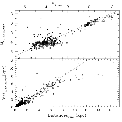
Figure 9: The same as Fig. 8 but for the full range of distances and absolute magnitudes. The dashed lines show one-to-one relations. The open squares indicate TO stars, filled diamonds BS–TO, open diamonds BS, filled squares MS, filled triangles SG, open triangles RG, filled inverted triangles RHB–AGB, open inverted triangles HB, filled circles BHB, open circles SL–BHB, and asterisks the SL stars. The comparison is shown for all VMP stars of this paper and of S96 for which distances have been derived from the two photometric systems.

During analyses and comparisons which followed those of this paper, a few possibly discrepant stars and their distances have come to light. For example, the distance of the RG star 22949–037 has been estimated at $\approx 14.7$ kpc from the $uvby$ photometry. This distance leads to very extreme Galactic velocities for this star, (U’,V’,W’) $\approx$ ($-622$, $-1420$, $-849$), probably implying that it is not bound to the Galaxy (see Fig. 1 of Garcia-Cole et al. 1999). A more likely explanation is that the $c_{\rm 0}$ index is distorted by large CNO overabundances (Depagne et al. 2002), leading to an unrealistic distance. (22949–037 has not been labeled as a CH star in Tables 3 and 5 since its medium-resolution spectrum of the HK survey did not extend far enough into the red to capture the G band.) The VMP RG star 29498–043 has similar overabundances of C and N (Aoki et al. 2002a, 2002b), and so its $uvby$ distance in Table 9 is probably similarly in error. The stars 30339–041 and 31083–069 have both been classified as RHB–AGB stars, but their $uvby$ photometry falls within the limits of our Hipparcos-based calibration giving $M_{\rm V}$ more like SG stars. The explanation here may be anomalous chemical abundances for AGB-like stars, binary contamination, or photometric variability, especially the latter for 31083–069 for which the SPM and La Silla $uvby$ observations do not agree well. The stars 29515–060 (classified MS) and 31081–003 (classified SG) have widely different $M_{\rm V}$ values from different methods which should be applicable, such as the Hipparcos-based calibration and the comparison with GCs. The former shows a difference $\Delta M_{\rm V}\approx 1\aas@@fstack{m}06$, and the latter $\approx 3\aas@@fstack{m}6$, and these differences may again imply anomalous chemical abundances or a binary companion for these two stars. As discussed above the $uvby$ data for 22955–032 can be used to appreciate the effects of photometric contamination by a nearby, fainter star; the three entries for this star show a range in $M_{\rm V}$ of nearly one magnitude and distance variations of nearly a factor of two.

7 Age comparisons

Figure 10 shows a $c_{\rm 0},(b$–$y)_{\rm 0}$ diagram comparing the VMP stars, the metal-poor GC M92, and isochrones from the work of Bergbusch & VandenBerg (2001). For the VMP stars, the dereddened photometry and classifications are taken from Table 5. The $uvby$ data for M92 is that of Grundahl et al. (2000a), as provided by Grundahl (2000), has been corrected for a reddening of $E(b-y)=0\aas@@fstack{m}016$, as suggested by these authors, and this CCD data has been plotted only for those stars with more than eight observations in the $u$–band and abs(SHARP) $\leq$ 0.05, from the DAOPHOT reduction package (Stetson 1987); this latter parameter measures the goodness of fit between the PSF of the object and the model PSF and is used to exclude non-stellar objects, double stars and stars affected by cosmic rays.

Also, the CCD $uvby$ data for M92 has been shifted by $-0\aas@@fstack{m}03$ in $c_{\rm 0}$, slightly less than the correction suggested by Grundahl et al. (2000a). They compared their $uvby$ data for M92 to that of local metal-poor stars from SN, especially the Hipparcos stars HD84937 and HD140283, using the $c_{\rm 0},(v-y)_{\rm 0}$ and M${}_{\rm V},(v-y)_{\rm 0}$ diagrams, and concluded that their $c_{\rm 0}$ values should be corrected by about $\approx-0\aas@@fstack{m}04$; they suspect that this problem is due to a $u$–band zero-point error. Indeed, in the $c_{\rm 0},(b$–$y)_{\rm 0}$ diagrams to follow (Figs. 10 and 11) we have noted a better overlap of the TO and SG distributions in $c_{\rm 0}$ if the M92 data is shifted downward by 0$\aas@@fstack{m}$02–0$\aas@@fstack{m}$03, slightly less than that recommended by Grundahl et al. (2000a).

This is surprising since the $uvby$ data of our VMP stars and that of the M92 stars should both be closely on the same photometric system, that of Olsen (1983, 1984), which is also that of SN. For the present catalogues the photometric standard stars were selected as described above, from Olsen (1983, 1984), from SN, and from S96. SN took great care to transform their $uvby$ data onto the system of Olsen (1983, 1984), and for the S96 catalogue the photometric standards were taken from Olsen and from SN. Grundahl et al. (2000a) also selected their 55 $uvby$ standard stars used to calibrate the M92 data from Olsen (1983, 1984) and from SN. So it all returns to that stated at the beginning of this paragraph: both sets of data (VMP and M92) should be closely on the standard $uvby$ system defined by Olsen (1983, 1984).

Plausibly, there might also be a shift in the relative $(b-y)$ systems as large as $0\aas@@fstack{m}01$ between the data of Grundahl et al. (2000a) and the present paper. However, the $(b-y)$ observations are usually the easiest to transform to the standard system of all the $uvby$ colors and indices, and these transformations are linear over a wide color range (Grønbech et al. 1976). For the photoelectric observations, typical instrumental errors in $(b-y)$ for the standard stars are $\pm 0\aas@@fstack{m}003$, and typical transformation dispersions, $\pm 0\aas@@fstack{m}005$. Systematic problems should be of this order or less.

The reddening value for M92 taken from Grundahl et al. (2000a) is the canonical value, and seems to be very well determined (Harris 1996, 2003; Schlegel et al. 1998). However, some authors (e.g. King et al. 1998) have argued for a much higher reddening for M92 ($0\aas@@fstack{m}09$–$0\aas@@fstack{m}10$) using indirect spectroscopic comparisons. Such a high reddening for M92 seems to be highly unlikely (VandenBerg 2000), but a possible error of $\pm 0\aas@@fstack{m}01$ in the canonical value cannot be ruled out, and should be kept in mind during the following relative-age comparisons.

In Fig. 10 clear evidence can be seen that the youngest VMP stars are somewhat younger than the GC M92. The upper extension along the isochrones of the VMP TO stars (the open squares) would indicate an age of 12–13 Gyrs, while the upper extent of M92, about 14.0–14.5 Gyrs for a difference of $\approx 1.5$–2.0 Gyrs. If one considers the transitional stars classified as BS–TO also as legitimate VMP turnoff stars, then 31066–027, plotted as a filled diamond with the values ($c_{\rm 0},(b$–$y)_{\rm 0}$, [Fe/H]) = (0$\aas@@fstack{m}$431, 0$\aas@@fstack{m}$262, $-2.11$), respectively, plus a couple of little-evolved TO stars, would indicate an even larger range of $\ga 2.0$–2.5 Gyrs between M92 and the youngest VMP stars. Our age for M92 agrees well with that derived by Grundahl et al. (2000a), 14.5 Gyrs, but we do not agree with them that “… the extremely metal-deficient field halo stars are most likely coeval with M92 to within 1 Gyr.” Other authors, such as Bell (1988), have also found that the bluest M92 stars are redder than the bluest VMP field subdwarfs, such as HD84937, by about 0$\aas@@fstack{m}$03 in $(B-V)_{\rm 0}$, corresponding to 0$\aas@@fstack{m}$02 in $(b-y)_{\rm 0}$ and an age difference of $\approx 2.5$ Gyrs, assuming similar metallicities.

However, these comparisons depend critically upon the [Fe/H] values used for the VMP field stars and for M92, i.e. upon the consistency between the [Fe/H] scale for field subdwarfs and VMP subgiants and the scale for GCs in which the metallicities have been measured mainly for the brighter red-giant stars. For example, Bergbusch & VandenBerg (2001) suggest that indeed there is an inconsistency between subdwarf and GC [Fe/H] scales based upon their fitting of isochrones to observed color-magnitude diagrams for GCs. More specifically, the above value of [Fe/H] $=-2.22$ for M92 has been obtained by Grundahl et al. (2000a) using sources based upon the high-resolution spectroscopy of the brighter red-giant stars and upon the calibration of the integrated light of GCs, while King et al. (1998) obtained [Fe/H] $=-2.52$ for M92 from high-resolution spectroscopic observations of three subgiants, a factor of two lower for the iron to hydrogen ratio. If this latter metallicity is indeed the correct one for M92, then in Fig. 10, VMP field stars with [Fe/H] $\approx-2.22$ are being compared to a GC with [Fe/H] $=-2.52$. According to the isochrones of Bergbusch & VandenBerg (2001), as transformed to $uvby$ by Clem et al. (2003), a correction for this metallicity difference would increase the age differences discussed above by about 1.5 Gyrs. A more recent study of the GC [Fe/H] scale by Kraft & Ivans (2003) suggests that at least part of the inconsistency with the subdwarf scale is due to non-LTE “overionization” effects for Fe I lines. For six red giants in M92 they obtain an average [Fe/H] = $-2.38$ from an analysis of Fe II lines only. Such a metallicity for M92 would require a correction of +0.8 Gyr to the age differences discussed above for Fig. 10.

In Fig. 11 the comparison of Fig. 10 is repeated, but now with the field VMP stars drawn from the range $-2.67<$ [Fe/H] $<-2.37$, which is centered on the value [Fe/H] $=-2.52$ for M92 obtained by King et al. (1998). This comparison would indicate age differences not that distinct from those of Fig. 10, despite the change in the mean metallicity of the field stars. Three TO stars along the axis of the isochrones would again suggest that the youngest VMP stars are 1.0–1.5 Gyrs younger than M92. The BS–TO star 22876–039 (0$\aas@@fstack{m}$486, 0$\aas@@fstack{m}$256, $-2.60$), and two little-evolved TO stars would indicate larger age differences, $\ga 3.0$ Gyrs.

These results are somewhat surprising, considering that M92 is among the more metal-poor and older GCs of the Galaxy (VandenBerg 2000), and that there is evidence that the formation of all metal-poor Galactic GCs was triggered throughout the Galaxy at the same time to within $\approx 1$ Gyr (Harris et al. 1997; Lee et al. 2001). Also, several previous studies (such as those of Pont et al. 1998 and of Grundahl et al. 2000a) have concluded that the more metal-poor field subdwarfs are coeval with M92 to within about 1 Gyr; however, these works have in general used only the more local subdwarfs, such as those from SN or Hipparcos. The VMP stars of this paper span a larger volume in the Galaxy, and the younger VMP stars of Figs. 10 and 11, which appear to be at least 1–3 Gyrs younger than M92, may reveal evidence for the belated formation of VMP stars outside of the Galactic GCs, the hierarchical infall of VMP material from the outermost parts of the proto-Galaxy after the GC system had formed (Sandage 1990), and/or the accretion of material from another galaxy with formation and chemical-enrichment histories different from that of the Galaxy (Preston et al. 1994; Ibata et al. 1994). For example, Preston et al. have concluded that their blue metal-poor stars ([Fe/H] $<-1.0$ and $0\aas@@fstack{m}15<(B-V)_{\rm 0}<0\aas@@fstack{m}35$, bluer than the GC turnoffs) are probably the result of accretion events by the Galaxy of material from dwarf galaxies, and the study of seven dwarf spheroidals by Dolphin (2002) has indeed shown recent (0.5–5 Gyrs) star formation for more than half of these (Carina, Leo I, Leo II, and Sagittarius), but higher metallicities ([Fe/H] $\approx-1.0$ to $-1.2$) than the present VMP stars. However, a previous compilation by Mateo (1998) gave [Fe/H] $\approx-1.9$ to $-2.0$ for Carina and Leo II, more in line with our VMP stars, but requiring an increase in the age estimates of Dolphin by $\approx 5$ Gyrs. Nevertheless, stars with [Fe/H] $\approx-2.0$ and ages of 5–10 Gyrs would come close to explaining the bluer VMP TO stars of Figs. 10 and 11.

Figure 10: Comparison in the $c_{\rm 0},(b$–$y)_{\rm 0}$ diagram of the VMP stars with $-2.42\leq$ [Fe/H] $\leq-2.02$ (with the same symbols as defined in Fig. 6), with the $uvby$ observations of M92 provided by Grundahl (2000a; points), and with the isochrones of Bergbusch & VandenBerg (2001) as transformed to $uvby$ photometry by Clem et al. (2003; solid curves). The isochrones are those for [Fe/H] $=-2.31$ and [$\alpha$/Fe] $=+0.30$, and have been plotted for 11, 12, 13, 14, and 15 Gyrs. The [Fe/H] of M92 has been taken here to be $-2.22$ according to the average derived by Grundahl et al. (2000a) from several high resolution spectroscopic studies of cluster giants found in the literature. Only those VMP stars with two or more $uvby$ observations have been plotted, and only those GC stars with more than eight $u$ observations and abs(SHARP) $\leq 0.05$. The M92 photometry has been shifted by $-0\aas@@fstack{m}03$ in $c_{\rm 0}$, similar to that correction suggested by Grundahl et al. (2000a).

Figure 11: The same $c_{\rm 0},(b$–$y)_{\rm 0}$ diagram as Fig. 10 but assuming that M92 has [Fe/H] $=-2.52$ according to the study of King et al. (1998) from high-resolution spectroscopy of three subgiants. The VMP stars are plotted for the range $-2.67\leq$ [Fe/H] $\leq-2.37$ (again with the same symbols as Fig. 6), with the same $uvby$ observations of M92 and with the same isochrones as in Fig. 10. Again, only those VMP stars with two or more $uvby$ observations have been plotted, and the M92 data has been shifted by $-0\aas@@fstack{m}03$ in $c_{\rm 0}$. Isochrones have been plotted for 11, 12, 13, 14, and 15 Gyrs.

8 Conclusions

1. The overall VMP HK-survey sample contains a wide range of stellar types, ranging from horizontal branch stars to subluminous, and from red giant stars to the blue horizontal branch.

2. The dereddened $c_{\rm 0},(b-y)_{\rm 0}$ diagram has been shown to be quite useful for providing photometric classifications of the VMP stars analogous to types derived from GC color-magnitude diagrams, such as Turn-Off stars (TO), SubGiants (SG), Red Giants (RG), Horizontal Branch stars (HB), Blue Horizontal Branch stars (BHB), Blue Stragglers (BS), SubLuminous stars (SL), and so forth (see Fig. 6).

3. The intrinsic-color calibration of Schuster & Nissen (1989), as modified slightly by Nissen (1994), is shown to provide reddening excesses, $E(b-y)$ or $E(B-V)$, very similar to the adopted reddening estimates derived in this publication from the maps of Schlegel, Finkbeiner, & Davis (1998) (see Eq. 1). No significant systematic offsets between these two dereddening techniques are noted (see Fig. 3).

4. A number of VMP stars have been noted with probable anomalous photometric traits, especially from the $m_{\rm 1}$ and $[m_{\rm 1}]$ indices; two such groups stand out. First, there are several stars with $(b$–$y)_{\rm 0}\la 0\aas@@fstack{m}45$ and with $m_{\rm 0}\ga 0\aas@@fstack{m}17$, much larger than would be expected for VMP stars with [Fe/H] $\la-1.5$. Most of these have been classified SG, and some show clear evidence of photometric variability. These are perhaps analogous to stars discussed in S96 with larger than expected $[m_{\rm 1}]$ values. We suggest here that these are misclassified AGB stars with unusual chemical-abundance ratios, photometric variability, and/or binary companions.

5. The second group of anomalous stars are those ten classified BS and having $m_{\rm 1}$, $[m_{\rm 1}]$, and $(U-B)_{\rm 0}$ values indicating nearly solar [Fe/H] values. There is a clear discrepancy here between these photometric indices and the KP index used to derive [Fe/H] for the HK survey. These stars are very similar to the Am stars identified by Wilhelm et al. (1999a, 1999b) and have been noted as “BS (Am)” in Table 5.

6. The photometric distances from the $UBV$ and $uvby$ photometries agree reasonably well considering the problems, lack of calibrating stars, and extrapolations needed for the more VMP stars. Our Hipparcos-based, photometric calibration for $M_{\rm v}$ seems to work quite well for the turn-off, main-sequence, and subgiant VMP stars, as suggested in Figs. 7 and 8.

7. In the $c_{\rm 0},(b-y)_{\rm 0}$ diagram, the youngest VMP stars appear to have ages 1–3 Gyrs younger than the GC M92. Uncertainties in the [Fe/H] scale for M92 would tend to increase this age difference even more. (The interstellar reddening of M92 seems to be well determined but might be as uncertain as $\pm 0\aas@@fstack{m}01$). Such younger VMP stars are showing evidence for important details upon the overall formation and evolution of the Galaxy, such as possible hierarchical star-formation/mass-infall for the VMP material, and/or accretion processes from other (dwarf) galaxies with different formation and chemical-enrichment histories.

- (1) Aoki, W., Norris, J. E., Ryan, S. G., Beers, T. C., & Ando, H. 2002a, ApJ, 576, L141
- (2) Aoki, W., Norris, J. E., Ryan, S. G., Beers, T. C., & Ando, H. 2002b, PASJ, 54, 933
- (3) Aoki, W., Ryan, S. G., Norris, J. E., Beers, T. C., Ando, H., & Tsangarides, S. 2002c, ApJ, 580, 1149
- (4) Anthony-Twarog, B. J., & Twarog, B. A. 1994, AJ, 107, 1577
- (5) Anthony-Twarog, B. J., Sarajedini, A., Twarog, B. A., & Beers, T. C. 2000, AJ, 119, 2882
- (6) Arce, H. G., & Goodman, A. A. 1999, ApJ, 512, L135
- (7) Beers, T. C. 1999, in Third Stromlo Symposium: The Galactic Halo, eds. B. Gibson, T. Axelrod, & M. Putman (ASP: San Francisco), 165, p. 206
- (8) Beers, T. C., Preston, G. W., & Shectman, S. A. 1985, AJ, 90, 2089 (BPSI)
- (9) Beers, T. C., Flynn, K., & Gebhardt, K. 1990, AJ, 100, 32
- (10) Beers, T. C., Preston, G. W., & Shectman, S. A. 1992, AJ, 103, 1987 (BPSII)
- (11) Beers, T. C., Rossi, S., Norris, J. E., Ryan, S. G., & Shefler, T. 1999, AJ, 117, 981
- (12) Beers, T. C., Chiba, M., Yoshii, Y., Platais, I., Hanson, R. B., Fuchs, B., & Rossi, S. 2000, AJ, 119, 2866
- (13) Bell, R. A. 1988, AJ, 95, 1484
- (14) Bergbusch, P. A., & VandenBerg, D. A. 2001, ApJ, 556, 322
- (15) Bonifacio, P., Monai, S., & Beers, T. C. 2000, AJ, 120, 2065
- (16) Brewer, J. & Storm, J. 1999, “Observing at the Danish 1.54-m telescope, A User’s Manual for the TCS and DFOSC”, ESO, La Silla, Chile
- (17) Budding, E. 1993, An Introduction to Astronomical Photometry (Cambridge University Press, Cambridge) 76
- (18) Burstein, D., & Heiles, C. 1982, AJ, 87, 1165
- (19) Busso, M., Gallino, R., & Wasserburg, G. J. 1999, ARA&A, 37, 239
- (20) Carney, B. W., Laird, J. B., Latham, D. W., & Aguilar, L. A. 1996, AJ, 112, 668
- (21) Christlieb, N. 2003, in Rev. in Modern Astronomy, 16, p. 191 (astro-ph/0308016)
- (22) Clem, J. L., VandenBerg, D. A., Grundahl, F., & Bell, R. A. 2003, AJ, submitted
- (23) Clementini, G., Carretta, E., Gratton, R., Merighi, R., Mould, J.R., & McCarthy, J. K. 1995, AJ, 110, 2319
- (24) Crawford, D. L. 1975a, PASP, 87, 481
- (25) Crawford, D. L. 1975b, AJ, 80, 955
- (26) Crawford, D. L. 1979, AJ, 84, 1858
- (27) Crawford, D. L., & Barnes, J. V. 1970, AJ, 75, 978
- (28) Crawford, D. L., & Mander, J. 1966, AJ, 71, 114
- (29) Depagne, E., Hill, V., Spite, M., et al. 2002, A&A, 390, 187
- (30) Doinidis, S. P., & Beers, T.C. 1990, PASP, 102, 1392
- (31) Doinidis, S. P., & Beers, T.C. 1991, PASP, 103, 973
- (32) Dolphin, A. E. 2002, MNRAS, 332, 91
- (33) ESA 1997, The Hipparcos and Tycho Catalogues, ESA SP–1200
- (34) Fujimoto, M. Y., Ikeda, Y., & Iben, I., Jr. 2000, ApJ, 529, L25
- (35) Garcia Cole, A., Schuster, W. J., Parrao, L., & Moreno, E. 1999, Rev. Mex. Astr. Astrofis., 35, 111
- (36) Gautschy, A., & Hideyuki, S. 1996, ARA&A, 34, 551
- (37) Girard, T. M., Dinescu, D. I., van Altena, W. F., Platais, I., Monet, D. G., & Lopez, C. E. 2003, AJ, submitted
- (38) Grønbech, B., Olsen, E. H., & Strömgren, B. 1976, A&AS, 26, 155
- (39) Grundahl, F. 2000, private communication
- (40) Grundahl, F., Briley, M., Nissen, P. E., Feltzing, S. 2002, A&A, 385, L14
- (41) Grundahl, F., VandenBerg, D. A., & Andersen, M. I. 1998, ApJ, 500, L179
- (42) Grundahl, F., VandenBerg, D. A., Bell, R. A., Andersen, M. I., & Stetson, P. B. 2000a, AJ, 120, 1884
- (43) Grundahl, F., VandenBerg, D. A., Stetson, P. B., Andersen, M. I., & Briley, M. 2000b, in: The Galactic Halo: From Globular Clusters to Field Stars, Proceedings of the 35th Liege International Astrophysics Colloquium, eds. A. Noels, P. Magain, D. Caro, E. Jehin, G. Parmentier, & A. A. Thoul, Liege, Belgium: Institut d’Astrophysique et de Geophysique
- (44) Hansen, C. J., & Kawaler, S. D. 1994, Stellar Interiors: Physical Principles, Structure, and Evolution (Springer-Verlag, New York)
- (45) Harris, W. 1994, A New Catalog of Globular Cluster Parameters, McMaster University
- (46) Harris, W. E. 1996, AJ, 112, 1487
- (47) Harris, W. E. 2003, “Catalogue of Milky Way Globular Cluster Parameters”, http://www.physics.mcmaster.ca/Globular.html
- (48) Harris, W. E., Bell, R. A., VandenBerg, D. A. et al. 1997, AJ, 114, 1030
- (49) Ibata, R. A., Gilmore, G., & Irwin, M. J. 1994, Nature, 370, 194
- (50) Johnson, H. L., Mitchell, R. I., Iriarte, B., & Wisniewski, W. Z. 1966, Comm. Lunar and Planetary Lab., No. 63, Univ. of Arizona, Tucson
- (51) King, J. R., Stephens, A., Boesgaard, A. M., & Deliyannis, C. P. 1998, AJ, 115, 666
- (52) Kraft, R. P., & Ivans, I. I. 2003, PASP, 115, 143
- (53) Kravtsov, V., Ipatov, A., Samus, N., Smirnov, O., Alcaíno, G., Liller, W., & Alvarado, F. 1997, A&AS, 125, 1
- (54) Lee, J. W., Carney, B. W., Fullton, L. K., & Stetson, P. B. 2001, AJ, 122, 3136
- (55) Mateo, M. 1998, ARA&A, 36, 435
- (56) Nissen, P. E. 1994, in: Stars, Gas and Dust in the Galaxy, Invited Reviews at a Symposium in Honor of Eugenio E. Mendoza, eds. A. Arellano Ferro & M. Rosado, Rev. Mex. Astr. Astrofis., 29, 129
- (57) Nissen, P. E., & Schuster, W. J. 1991, A&A, 251, 457
- (58) Norris, J. E., Ryan, S. G., & Beers, T. C. 1997, ApJ, 488, 350
- (59) Olsen, E. H. 1983, A&AS, 54, 55
- (60) Olsen, E. H. 1984, A&AS, 57, 443
- (61) Pilachowski, C. A., Sneden, C., & Booth, J. 1993, ApJ, 407, 699
- (62) Pont, F., Mayor, M., Turon, C., & VandenBerg, D. A. 1998, A&A, 329, 87
- (63) Preston, G. W., Shectman, S.A., & Beers, T. C. 1991, ApJS, 76, 1001
- (64) Preston, G. W., Beers, T. C., & Shectman, S. A. 1994, AJ, 108, 538
- (65) Rey, S., Yoon, S., Lee, Y., Chaboyer, B., & Sarajedini, A. 2001, AJ, 122, 3219
- (66) Rossi, S., Beers, T. C., & Sneden, C. 1999, in Third Stromlo Symposium: The Galactic Halo, eds. B. Gibson, T. Axelrod, & M. Putman (ASP Conference Series), 165, p. 268
- (67) Ryan, S. G., & Norris, J. E. 1991, AJ, 101, 1835
- (68) Sandage, A. 1990, J. Roy. Astron. Soc. Canada, 84, 70
- (69) Schlattl, H., Salaris, M., Cassisi, S., & Weiss, A. 2002, A&A, 395, 77
- (70) Schlegel, D. J., Finkbeiner, D. P., & Davis, M. 1998, ApJ, 500, 525
- (71) Schuster, W. J., & Nissen, P. E. 1988, A&AS, 73, 225 (SN)
- (72) Schuster, W. J., & Nissen, P. E. 1989, A&A, 221, 65
- (73) Schuster, W. J., Nissen, P. E., Parrao, L., Beers, T. C., & Overgaard, L. P. 1996, A&AS, 117, 317 (S96)
- (74) Schuster, W. J., Parrao, L., & Contreras Martínez, M. E. 1993, A&AS, 97, 951 (SPC)
- (75) Schuster, W. J., & Parrao, L. 2001, Rev. Mex. Astr. Astrofis., 37, 187
- (76) Stetson, P. B. 1987, PASP, 99, 191
- (77) Strömgren, B. 1966, ARA&A, 4, 443
- (78) VandenBerg, D. A. 2000, ApJS, 129, 315
- (79) Villeneuve, B., Wesemael, F., & Fontaine, G. 1995, ApJ, 450, 851
- (80) Weidemann, V. 1968, ARA&A, 6, 351
- (81) Wesemael, F., Fontaine, G., Bergeron, P., Lamontagne, R., & Green, R. F. 1992, AJ, 104, 203
- (82) Wilhelm, R., Beers, T. C., & Gray, R. 1999a, AJ, 117, 2308
- (83) Wilhelm, R., Beers, T. C., Sommer-Larsen, J., Pier, J. R., Layden, A. C., Flynn, C., Rossi, S., & Christensen, P. R. 1999b, AJ, 117, 2329
- (84) Zacharias, N. 2002, in Survey and Other Telescope Technologies and Discoveries, eds. J. A. Tyson & S. Wolff (Proc. of the SPIE), 4836, p. 279
- (85) Zac̆s, L., Nissen, P. E., & Schuster, W. J. 1998, A&A, 337, 216