The Scaleheight of Giant Molecular Clouds is
Less than that of Smaller Clouds

Abstract

We have used an antenna temperature thresholding algorithm on the Bell Laboratories ${}^{13}\mathrm{CO}$ Milky Way Survey to create a catalog of 1,400 molecular clouds. Of these, 281 clouds were selected for having well-determined kinematic distances. The scaleheight, luminosity, internal velocity dispersion, and size of the cloud sample are analyzed to show that clouds smaller than $\sim 10^{5.5}\,\mathrm{M_{\odot}}$ have a scaleheight which is about 35 pc, roughly independent of cloud mass, while larger clouds, the Giant Molecular Clouds, have a reduced scaleheight which declines with increasing cloud mass.

1 Introduction

Since star formation occurs in molecular clouds, the formation of molecular clouds is an essential first step to the star formation process. The overall evolution of galactic metallicity implies that hot ejecta from old stars must somehow return to the cold molecular phase in order to form new stars, and that the timescale for this process is short compared to the age of the Galaxy (e.g. Freeman & Bland-Hawthorn, 2002). Giant Molecular Clouds (GMCs) are the largest concentrations of molecular material, amounting to $2\times 10^{5}\mathrm{M_{\odot}}$ or more in a region about 50 pc in size (Stark & Blitz, 1978). GMCs are strongly concentrated to spiral arms (Stark, 1979; Lee et al., 2001), suggesting that they are transient phenomena: hundreds of thousands of solar masses of molecular material collect during the passage of a spiral density wave, and then dissipate some thirty million years later. Thousands of stars are formed during the lifetime of the GMC, including the generators of the giant H II regions that trace spiral structure. How molecular clouds form, and why they form, has been the subject of ongoing theoretical investigation (Elmegreen, 2000; Pringle et al., 2001). Computer simulations of cloud formation have become increasingly complex and realistic (Hartmann et al., 2001; Zhang et al., 2002).

The cloud formation process gathers and concentrates interstellar matter. However this happens, we expect that the random velocity of the resulting cloud would be less than the velocity dispersion of the precursor material, so that the velocity dispersion of GMCs as a class would be less than that of smaller interstellar clouds. This hypothesis is amenable to observational test. The purpose of this Letter is to describe such an observational test, and then to quantify the effect in a way which may make for useful comparisons with theory.

In §2, we take the Bell Laboratories ${}^{13}\mathrm{CO}$ Survey data and use a brightness temperature thresholding algorithm to create a catalog of molecular clouds. We then use our knowledge of Milky Way structure in order to select a subset of clouds with well-determined kinematic distances. This allows us to determine the physical size of the cloud and its distance above the galactic plane. These data are analyzed in §3 to show that the scaleheight of large clouds is less than that of smaller clouds.

2 Cloud Identification and Selection

The version of Bell Laboratories ${}^{13}\mathrm{CO}$ Survey used here is described by Lee et al. (2001). The survey covers 244 square degrees from $\ell=-5{{}^{\circ}}\,{\mathrm{to}}\,117{{}^{\circ}}$, $b=-1{{}^{\circ}}\,{\mathrm{to}}\,+1{{}^{\circ}}$ sampled on a $3^{\prime}$ or $6^{\prime}$ grid with ${}^{13}\mathrm{CO}$ spectra having an rms noise level of $T_{R}^{*}=0.1\,{\mathrm{K}}$ in channels $0.68\,{\mathrm{km\,s^{-1}}}$ wide. The survey data consists of 23 million data points (pixels) in a 3-dimensional $(\ell,\,b,\,v)$ space; these are shown in Lee et al. (2001) as a series of $\ell$—$v$ maps. The survey is not fully sampled, but it is sufficiently well-sampled that no cloud within the survey volume larger than $\sim 1\times 10^{3}\mathrm{M_{\odot}}$ would be missed due to undersampling.

Catalogs of clouds were generated from the survey data by a standard thresholding technique (Solomon et al., 1987; Lee et al., 1990; Lee, 1992). In this method, pixels having $T_{R}^{*}>T_{\mathrm{th}}$ are identified for some value of a threshold brightness temperature $T_{\mathrm{th}}$. The value of $T_{\mathrm{th}}$, typically 1, 2, or 3 K, is the defining parameter of the catalog. Pixels exceeding the threshold are then grouped together in $(\ell,\,b,\,v)$ space to make a “cloud”, where all the pixels constituting the cloud are above the threshold and adjacent to at least one other pixel which is also above the threshold. What we mean by a “cloud” is then a connected volume of pixels, all of which are above the threshold. This cloud recognition method has the advantage of non-subjectivity—not only is it automated and unambiguous, it makes no assumptions about cloud properties aside from the requirement that a cloud be a connected region which is brighter than its surroundings. A disadvantage of the thresholding method is that physically separated molecular clouds can be bundled together into a single catalog entry if they are projected onto each other such that above-threshold pixels within them appear to touch from our point of view. This happens more often for small values of $T_{\mathrm{th}}$. If the clouds are truly unassociated, the resulting catalog entry will be systematically too large and have too high an internal velocity dispersion. Another disadvantage is that all emission below $T_{\mathrm{th}}$ is discarded, cutting off the outer envelopes of the clouds and systematically underestimating their total emissivity and extent. This happens more often for large values of $T_{\mathrm{th}}$. A choice of $T_{\mathrm{th}}=1\mathrm{K}$ for our ${}^{13}\mathrm{CO}$ data is an acceptable compromise. This is approximately $10\times$ the rms noise level of the survey; since we require that a “cloud” be at least two pixels wide in each of the three dimensions $(\ell,\,b,\,v)$, there are probably no cloud catalog entries referring to non-existent clouds. Fewer than 1% of survey pixels exceed the 1 K threshold, as discussed in §2 of Lee et al. (2001), so the number of above-threshold adjacencies occurring by chance will be small. Applying the thresholding method with $T_{\mathrm{th}}=1\mathrm{K}$ on the Bell Laboratories ${}^{13}\mathrm{CO}$ Survey yields a catalog of 1,400 clouds.

We know the position of each cloud in $(\ell,\,b,\,v)$, but we would also like to know its distance along the line of sight in order to estimate its size and its height above the galactic plane. That can be done, to a greater or lesser extent, by fitting the cloud’s position in $(\ell,\,b,\,v)$ to our knowledge of the velocity field of the Galaxy. Many molecular clouds are on a nearly circular orbit around the Galactic Center at a velocity which differs little from $\Theta=215\,{\mathrm{km\,s^{-1}}}$, the rotation curve velocity. Other clouds, particularly those near the Galactic Center, can have significant non-circular motions. For each cloud, there are various possible distances, given our knowledge of motions in the Milky Way. We can quantify this situation by considering the set of possible distances. Consider first the simple case of a cloud in the second quadrant at $\ell=110{{}^{\circ}}$, $b=0{{}^{\circ}}$ and $v=-20\,{\mathrm{km\,s^{-1}}}$. It is most likely to be at the point 2 kpc distant along the line of sight corresponding to circular motion at that position and velocity, since its total velocity probably does not deviate from the rotation velocity by more than the typical cloud-cloud velocity dispersion. We can set approximate limits to range of possible distances by first adding, then subtracting, the one-dimensional velocity dispersion of $7\,{\mathrm{km\,s^{-1}}}$ (Stark & Brand, 1989) from its observed velocity, finding that it is likely no more than 2.6 kpc distant nor less than 1.3 kpc distant. Next, consider a cloud in the first quadrant at, e.g., $l=30{{}^{\circ}}$, which will have two ranges of possible distances because of the rotation curve distance ambiguity, resulting in four endpoints to the two (possibly overlapping) ranges of distances. Another cloud with a large velocity which is projected onto the Galactic Center could be anywhere from 6 to 10 kpc distant. Any cloud with a small velocity ($|v|<14\,{\mathrm{km\,s^{-1}}}$) at any longitude could be as near as 0.15 kpc or as distant as 1 kpc, or could be at other distances permitted by the galactic rotation at its longitude and velocity. Table 1 lists the ranges of possible distances for clouds in various regions of $(\ell,\,v)$ space. Each cloud will fall within one or more of these regions, resulting in a cumulative set of several possible distances. Call the largest member of that set $d_{\mathrm{far}}$, and the smallest member $d_{\mathrm{near}}$. These values serve as approximate bounds on the distance to the cloud, but they are not Gaussian errors—in most cases, the true distance will be somewhere between these values, but the distribution of true distances may be bimodal or asymmetric. These limits do, however, allow us to select a subset of the data whose distance ambiguity is not too large.

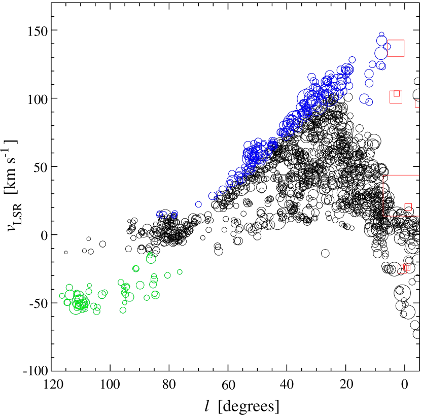
Figure 1: Distribution in $\ell$ and $v$ of 1400 clouds from a cloud catalog with $T_{th}=1\,\mathrm{K}$ made from the Bell Laboratories ${}^{13}\mathrm{CO}$ Survey. The linear size of each symbol is proportional to the velocity width of the corresponding cloud. The 218 clouds which satisfy our distance accuracy requirement are shown in color: red squares for Galactic Center clouds, blue circles for the molecular ring tangent velocities, and green circles for outer Galaxy clouds.

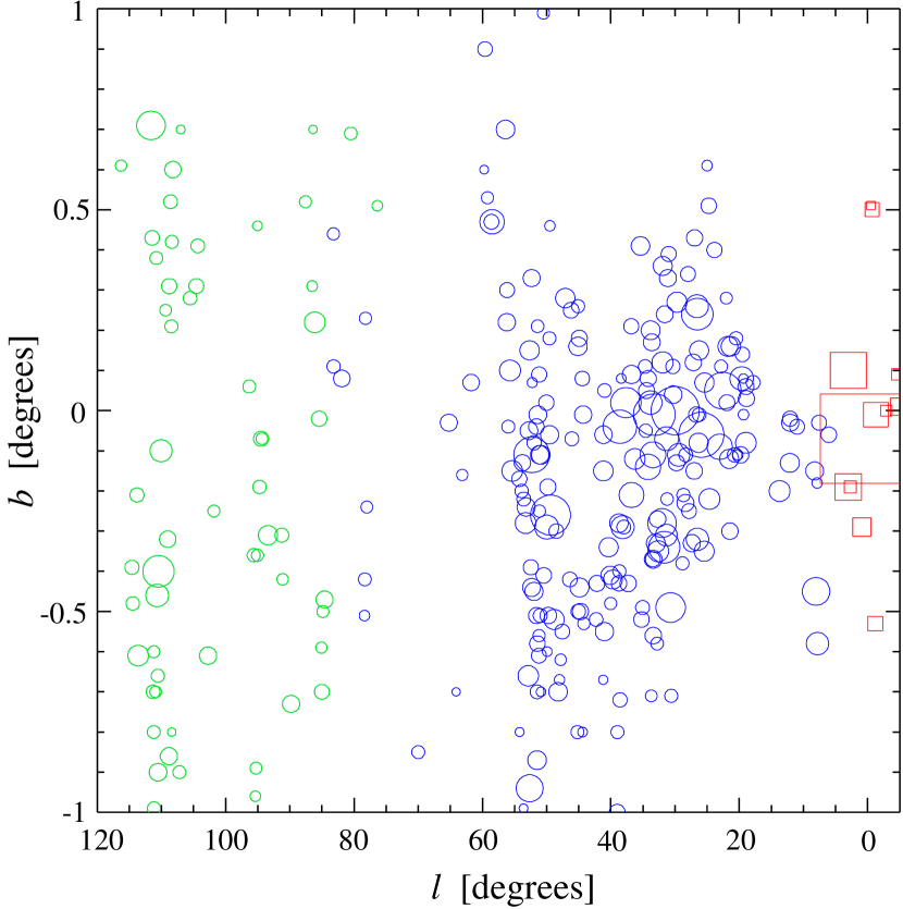
Figure 2: Distribution in $\ell$ and $b$ of 281 distance-selected clouds. The clouds are color coded as in figure 1. Note that the clouds as they appear on the sky are very much smaller than the size of the symbols used here, especially in the $\ell$ direction, and that the clouds are also separated in velocity. Chance superposition of clouds is therefore unlikely. The limit of the survey in $b$ probably cuts off some clouds which should be in the sample.

In the analysis below, we select only those clouds for which $d_{\mathrm{far}}/d_{\mathrm{near}}<\sqrt{3}$. This limit is sufficiently large that it does not exclude all clouds in the Galactic Center region. Since luminosity varies as $d^{2}$, the ambiguity in the luminosity of the distance-selected clouds is less than a factor of 3, and so we know their luminosity within half an order of magnitude. The distance-selected clouds are shown in color in figure 1. The selected sample consists of 281 clouds, and they come from three general locations: the Perseus arm (at $\ell>80{{}^{\circ}}$ and $v<-14\,{\mathrm{km\,s^{-1}}}$), the first quadrant near the tangent velocity, and the Galactic Center. Most of these clouds are several kiloparsec distant. This is good, because one source of bias in the analysis below comes from the limited range of the survey in galactic latitude, $|b|<1{{}^{\circ}}$. We do not want this limit to exclude many clouds that would otherwise be in the sample, and that will be true only if most of the selected clouds are distant. Figure 2 shows that only a few of the distance-selected clouds are near the $b$ limit of the survey, while the unselected set of survey clouds have a larger range and fill the survey space.

3 Cloud Scaleheights

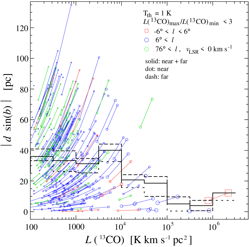
Figure 3: Scaleheight vs. luminosity for 281 molecular clouds selected for small distance uncertainty. Each cloud is shown at its near distance and its far distance, and these symbols are joined by a line. The data points are averaged into bins half an order of magnitude wide. The averages are shown as three histograms: the dotted line includes only the near distance values, the dashed line includes only the far distance values, and the solid line includes both. The linear dimension of each symbol is proportional to the cloud’s linewidth.

The scaleheights of the distance-selected sample are shown in figure 3, as a function of cloud luminosity. Each cloud is shown twice, once for the values corresponding to $d_{\mathrm{near}}$, and once for the values corresponding to $d_{\mathrm{far}}$. These points are connected by a line. The true values for each cloud probably lies somewhere near that line. Here we have chosen to simply define scaleheight as the height above the galactic equator at $b=0{{}^{\circ}}$, rather than try to better define the galactic midplane. Also shown in this plot are three very similar histograms, where the scaleheights have been averaged in bins an order of magnitude wide in ${}^{13}\mathrm{CO}$ luminosity. The dotted histogram only includes values of $d_{\mathrm{near}}$, the dashed histogram only includes values of $d_{\mathrm{far}}$, and the solid histogram includes both. The essential similarity of these three histograms shows that in the current sample of 281 clouds, the remaining distance ambiguities are not important to the result. For small, low luminosity clouds, the scaleheight is roughly constant at 35 pc, independent of cloud size. This value may be systematically small because of the cutoff at $b=\pm 1{{}^{\circ}}$, but it is not significantly different from the scaleheight of the overall CO brightness distribution found by Malhotra (1994b) using data with a much larger range in $b$. Note that at a cloud luminosity of about $10^{4}\,\mathrm{K\,{\mathrm{km\,s^{-1}}}\,pc^{2}}$, there is a break in the distribution and the larger clouds have a reduced scaleheight of about 20 pc for clouds in the range $L(^{13}\mathrm{CO})=10^{4}$ to $10^{5}\,\mathrm{K\,{\mathrm{km\,s^{-1}}}\,pc^{2}}$, and 5 or 10 pc for the few clouds brighter than $10^{5}\,\mathrm{K\,{\mathrm{km\,s^{-1}}}\,pc^{2}}$. For the largest clouds, the derived scaleheight is smaller than the cloud’s size and the galactic midplane falls within the boundary of the cloud.

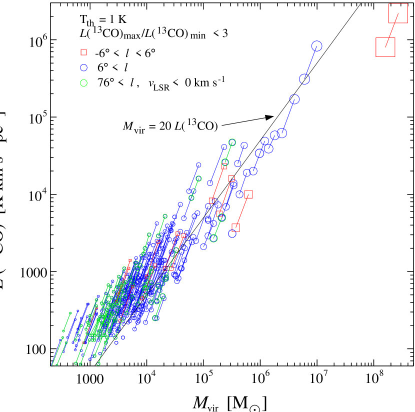
Figure 4: Luminosity in ${}^{13}\mathrm{CO}$ vs. estimated virial mass for the 281 molecular clouds selected for small distance uncertainty. The linear dimension of each symbol is proportional to the cloud’s linewidth. Galactic Center objects are shown as squares. The line $M_{\mathrm{vir}}=20\,L(^{13}\mathrm{CO})$ is shown for reference.

Since ${}^{13}\mathrm{CO}$ is in general not optically thick in these clouds, the ${}^{13}\mathrm{CO}$ luminosity will be approximately proportional to cloud mass (Lee, 1994). This is illustrated in figure 4, where the luminosity of the clouds in this sample is plotted against an estimate of the mass obtained from the linewidth and the cloud size. What we have done here is to ignore all terms in the magnetohydrodynamic virial equation (Spitzer, 1978) except for the kinetic and potential energy volume integrals. This is likely to be a valid approximation, since the internal pressure in molecular clouds is higher than the surrounding medium, the internal magnetic pressure is in approximate equipartition with other pressures, and the timescale for large-scale dissipation of the clouds is somewhat greater than a free-fall time. The absence of serious outliers in figure 4 is further evidence that the GMCs in our sample are real objects and not chance superpositions of small clouds. The data are well-represented by the relation $M_{\mathrm{vir}}=[20\,\mathrm{\mathrm{M_{\odot}}/K\,km\,s^{-1}}]L(^{13}\mathrm{CO})$, which corresponds to a galactic conversion factor (e.g., Sanders et al., 1984) $X(^{13}\mathrm{CO})=1.25\times 10^{21}\mathrm{cm^{-2}/K\,km\,s^{-1}}$. The scaleheight breakpoint at a luminosity of $10^{4}\,\mathrm{K\,{\mathrm{km\,s^{-1}}}\,pc^{2}}$ is therefore seen to correspond to a cloud mass $\sim 2\times 10^{5}\mathrm{M_{\odot}}$, the size of a small GMC. The scaleheight of GMCs is less than that of smaller clouds.

4 Conclusion

The data show that small molecular clouds have a scaleheight which is approximately independent of cloud size. Larger clouds, the GMCs, have a scaleheight which falls off with mass. This has been demonstrated with a relatively small sample of clouds, but it is a clean sample, chosen from a large-scale survey by an algorithmic method. The implication is that the Giant Molecular Clouds, those clouds which are concentrated in the spiral arms of the Galaxy, are also concentrated to the galactic plane. We can understand this as a manifestation of the molecular cloud formation process. Atomic gas clouds, with a scaleheight of $\sim 100\,\mathrm{pc}$ and a velocity dispersion $\sim 12\,{\mathrm{km\,s^{-1}}}$, condense out of the diffuse atomic gas. Their cores become molecular and increasingly more condensed, resulting in a population of high-latitude ($\sim 70\,\mathrm{pc}$), low mass ($M\mathrel{\raise 1.50696pt\hbox{$\scriptstyle<$}\kern-6.00006pt\lower 1.72218pt\hbox{{$\scriptstyle\sim$}}}100\,\mathrm{M_{\odot}}$) partially-molecular clouds with a dispersion $\sim 8\,{\mathrm{km\,s^{-1}}}$ (Malhotra, 1994a; Dame & Thaddeus, 1994). These clouds become larger, more centrally condensed, and more bound, with only a slight reduction in scaleheight and velocity dispersion, to become molecular clouds ($100\,\mathrm{M_{\odot}}\mathrel{\raise 1.50696pt\hbox{$\scriptstyle<$}\kern-6.00006pt\lower 1.72218pt\hbox{{$\scriptstyle\sim$}}}M\mathrel{\raise 1.50696pt\hbox{$\scriptstyle<$}\kern-6.00006pt\lower 1.72218pt\hbox{{$\scriptstyle\sim$}}}10^{5}\,\mathrm{M_{\odot}}$), with dispersion $\sim 7\,{\mathrm{km\,s^{-1}}}$ (Stark & Brand, 1989). These clouds can form stars, but are uniformly distributed throughout the galactic disk, and may survive for many galactic rotations. The largest clouds, the GMCs, are rapidly assembled by the passage of a spiral arm. This process is dissipative, different from the slow addition of material that forms smaller molecular clouds. It results in a significant loss of random velocity per unit mass, and the resulting GMCs are found at the galactic midplane, in the spiral arm. The ensuing formation of massive stars destroys the cloud, fragmenting it into stars, ionized gas, and small clouds before the next interarm passage.

Table 1: Possible cloud distances.

Location	$\ell$	$v$	Possible Distances
all	any	any	$R_{\sun}\left(\mathrm{cos}\,\ell\,+\,\sqrt{\mathrm{sin^{2}}\,\ell\,[({v\over\Theta}+\mathrm{sin}\,\ell\,)^{-2}-1]}\,\right)$  ,
			$R_{\sun}\left(\mathrm{cos}\,\ell\,+\,\sqrt{\mathrm{sin^{2}}\,\ell\,[({{v+v_{\sigma}}\over\Theta}+\mathrm{sin}\,\ell\,)^{-2}-1]}\,\right)$  ,
			$R_{\sun}\left(\mathrm{cos}\,\ell\,+\,\sqrt{\mathrm{sin^{2}}\,\ell\,[({{v-v_{\sigma}}\over\Theta}+\mathrm{sin}\,\ell\,)^{-2}-1]}\,\right)$
$1^{\mathrm{st}}$ and $4^{\mathrm{th}}$ quandrants	$|\ell\,|<90{{}^{\circ}}$	$v\,\mathrm{sin}\,\ell\,>0$	$R_{\sun}\left(\mathrm{cos}\,\ell\,-\,\sqrt{\mathrm{sin^{2}}\,\ell\,[({v\over\Theta}+\mathrm{sin}\,\ell\,)^{-2}-1]}\,\right)$  ,
			$R_{\sun}\left(\mathrm{cos}\,\ell\,-\,\sqrt{\mathrm{sin^{2}}\,\ell\,[({{v+v_{\sigma}}\over\Theta}+\mathrm{sin}\,\ell\,)^{-2}-1]}\,\right)$  ,
			$R_{\sun}\left(\mathrm{cos}\,\ell\,-\,\sqrt{\mathrm{sin^{2}}\,\ell\,[({{v-v_{\sigma}}\over\Theta}+\mathrm{sin}\,\ell\,)^{-2}-1]}\,\right)$
Galactic Center region	$|\ell\,|<8{{}^{\circ}}$	any	${5\over 4}R_{\sun}\,$,
			${3\over 4}R_{\sun}$
3 kpc arm	$|\ell\,|<11{{}^{\circ}}$	$5\ell-61{{}^{\circ}}<{v\over{1\,{\mathrm{km\,s^{-1}}}}}<5\ell-41{{}^{\circ}}$	${5\over 8}R_{\sun}$
$135\,{\mathrm{km\,s^{-1}}}$ arm	$|\ell\,|<5{{}^{\circ}}$	$5\ell+125{{}^{\circ}}<{v\over{1\,{\mathrm{km\,s^{-1}}}}}<5\ell+145{{}^{\circ}}$	${11\over 8}R_{\sun}$
solar vicinity	any	$|v|<2v_{\sigma}$	0.15 kpc,
			1 kpc

Note. — The galactic parameters used are: the Sun’s distance to the Galactic Center, $R_{\sun}=8\,\mathrm{kpc}$, the velocity of the flat rotation curve, $\Theta=215\,{\mathrm{km\,s^{-1}}}$, and the one-dimensional velocity dispersion of molecular clouds, $v_{\sigma}=7\,{\mathrm{km\,s^{-1}}}$. Galactic longitude, $\ell$, expressed in degrees, ranges from $-180{{}^{\circ}}$ to $+180{{}^{\circ}}$. Any possible distances which are not positive real numbers are discarded.

References

- Dame & Thaddeus (1994) Dame, T. M. & Thaddeus, P. 1994, ApJ, 436, L173
- Elmegreen (2000) Elmegreen, B. G. 2000, ApJ, 530, 277
- Freeman & Bland-Hawthorn (2002) Freeman, K. & Bland-Hawthorn, J. 2002, ARA&A, 40, 487
- Hartmann et al. (2001) Hartmann, L., Ballesteros-Paredes, J., & Bergin, E. A. 2001, ApJ, 562, 852
- Lee (1992) Lee, Y. 1992, PhD thesis, University of Massachusetts
- Lee (1994) Lee, Y. 1994, Publication of Korean Astronomical Society, 9, 55
- Lee et al. (1990) Lee, Y., Snell, R. L., & Dickman, R. L. 1990, ApJ, 355, 536
- Lee et al. (2001) Lee, Y., Stark, A. A., Kim, H.-G., & Moon, D.-S. 2001, ApJS, 136, 137
- Malhotra (1994a) Malhotra, S. 1994a, ApJ, 437, 194
- Malhotra (1994b) —. 1994b, ApJ, 433, 687
- Pringle et al. (2001) Pringle, J. E., Allen, R. J., & Lubow, S. H. 2001, MNRAS, 327, 663
- Sanders et al. (1984) Sanders, D. B., Solomon, P. M., & Scoville, N. Z. 1984, ApJ, 276, 182
- Solomon et al. (1987) Solomon, P. M., Rivolo, A. R., Barrett, J., & Yahil, A. 1987, ApJ, 319, 730
- Spitzer (1978) Spitzer, Jr., L. 1978, Physical Processes in the Interstellar Medium (John Wiley & Sons)
- Stark (1979) Stark, A. A. 1979, PhD thesis, Princeton University
- Stark & Blitz (1978) Stark, A. A. & Blitz, L. 1978, ApJ, 225, L15
- Stark & Brand (1989) Stark, A. A. & Brand, J. 1989, ApJ, 339, 763
- Zhang et al. (2002) Zhang, T., Song, G., Yang, Z., Chen, L., Zhang, B., Li, N., & Cui, J. 2002, Chinese Astronomy and Astrophysics, 26, 276