A comprehensive set of simulations of high-velocity collisions between main sequence stars.

Abstract

We report on a very large set of simulations of collisions between two main sequence (MS) stars. These computations were done with the “Smoothed Particle Hydrodynamics” method. Realistic stellar structure models for evolved MS stars were used. In order to sample an extended domain of initial parameters space (masses of the stars, relative velocity and impact parameter), more than 14 000 simulations were carried out. We considered stellar masses ranging between 0.1 and $75\,{\rm M}_{\odot}$ and relative velocities up to a few thousands $\mathrm{km\,s}^{-1}$. To limit the computational burden, a resolution of 1000–32 000 particles per star was used. The primary goal of this study was to build a complete database from which the result of any collision can be interpolated. This allows us to incorporate the effects of stellar collisions with an unprecedented level of realism into dynamical simulations of galactic nuclei and other dense stellar clusters. We make the data describing the initial condition and outcome (mass and energy loss, angle of deflection) of all our simulations available on the Internet. We find that the outcome of collisions depends sensitively on the stellar structure and that, in most cases, using polytropic models is inappropriate. Published fitting formulae for the collision outcomes, established from a limited set of collisions, prove of limited use because they do not allow robust extrapolation to other stellar structures or relative velocities.

1 Introduction

1.1 Stellar collisions in galactic nuclei

Figure 1: Relaxation and collision times at 0.1 pc from a massive black hole in the centre of a galactic nucleus (inspired from a similar diagram by Arabadjis 1997). We plot curves of iso-$T_{\mathrm{relax}}$ (dashes, blue in colour version) and iso-$T_{\mathrm{coll}}$ (solid lines, magenta in colour version) in a plane parameterised by the stellar density at 0.1 pc and the mass of the central black hole. The right ordinate scale indicates the stellar velocity dispersion (Keplerian value, $\sigma_{V}=\sqrt{GM_{\rm BH}/r}$). All stars are assumed to be of solar type. The left shaded sector (cyan in colour version) corresponds to conditions for which both $T_{\mathrm{relax}}$ and $T_{\mathrm{coll}}$ are larger than Hubble time, so that such nuclei are not expected to show signs of secular evolution. In the shaded lower right corner, the black hole does not dominate the kinematics and the effect of the cluster’s self gravitation should be included in the computation of the characteristic time-scales.
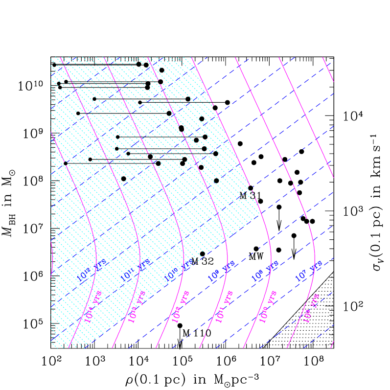
Large black dots show the estimated conditions for observed galactic nuclei. In most cases, the estimation of the stellar density at 0.1 pc requires important extrapolation from the data, as such a small radius is resolved only for a few galaxies of the local group (the Milky Way, M 31 and M 32). For this extrapolation, we use a power-law cusp of the form $\rho(r)=\rho_{0}(r_{0}/r)^{\gamma}$. The values of $\rho_{0}$, $r_{0}$ and $\gamma$ are taken from Gebhardt et al. (2003) or Faber et al. (1997). The densities for M 31 and M 32 are from Lauer et al. (1998) and the Milky Way’s value from Genzel et al. (1996). The values of $M_{\mathrm{BH}}$ are estimates by Magorrian et al. (1998), van der Marel (1999) or better constrained values gathered by Kormendy (2004, see http://chandra.as.utexas.edu/~kormendy/bhsearch.html for these data and a list of original references). In some cases, $\rho_{0}$ and $r_{0}$ have already been extrapolated from larger radii! Cases with an horizontal line connected to a second smaller dot are nuclei for which the slope $\gamma$ is observational compatible with $0$, according to Faber et al. (1997). The second point indicates the density value at 0.1 pc if constant $\rho$ is assumed up to $r_{0}$.

In the recent years, the study of stellar collisions has received renewed interest from researchers studying the dynamics of dense stellar systems, either open/globular clusters or galactic central regions (see the contributions in Shara 2002). Our own motivation is to perform simulations of the long-term evolution of dense stellar systems, particularly galactic nuclei, with a new Monte Carlo stellar dynamics code which incorporate collisions as “micro-physics” (Freitag & Benz, 2001b, 2002).

Before going into a brief description of the astrophysical motivations of these works, some clarification about the notion of “stellar collision” is called for. In this paper we shall use this term to refer to a process during which two stars, previously unbound to each other, get so close that not only gravitational forces but also hydrodynamical ones come into play to determine the outcome of the interaction. So, strictly speaking, collisions are not only contact encounters but also comprise tidal interactions. However, for reasons to be exposed in Sec. 2.8, we restrict here to events leading to physical contact at first periastron passage.

To assess the importance of collisions in a given astrophysical context, the key quantity to monitor is the collision time, which we define here as the average time needed for “test-star” 1 to experience a collision with any “field-star” 2,

$$T_{\mathrm{coll}} = \left(n_{2}Sv_{\mathrm{rel}}\right)^{-1}$$ (1)

$$\mbox{with\ }S = \pi d_{\mathrm{coll}}^{2}\left(1+\frac{2G(M_{1}+M_{2})}{d_{\mathrm{coll}}v_{\mathrm{rel}}^{2}}\right),$$ (2)

where $n_{2}$ is the number density of the field stars, $v_{\mathrm{rel}}$ the relative velocity and $d_{\mathrm{coll}}$ the pericentre distance leading to a collision ($d_{\mathrm{coll}}=R_{1}+R_{2}$ for contact at first passage, neglecting tidal deformation). $S$ is the collisional cross-section. At low relative velocity, it is greatly enhanced over the geometric value by gravitational attraction. This effect, dubbed “focusing” is expressed by the second term in the brackets of Eq. 2. In most astronomical contexts, the velocity dispersion is much smaller than the stellar escape velocity $V_{\star}=\sqrt{2GM_{\star}/R_{\star}}$ ($\simeq 620$ $\mathrm{km\,s}^{-1}$ for sun-like stars) and gravitational focusing dominates. In these cases, integrating over a Maxwellian distribution for relative velocities yields (Binney & Tremaine, 1987, Eq. 8–125):

$$T_{\mathrm{coll}} \simeq 7\times 10^{14}\,\mathrm{yrs}\,\times$$

$$\left(\frac{R_{\star}}{{{\rm R}_{\odot}}}\right)^{-1}\left(\frac{M_{\star}}{{{\rm M}_{\odot}}}\right)^{-1}\left(\frac{n}{\mathrm{pc}^{-3}}\right)^{-1}\left(\frac{\sigma_{v}}{\mathrm{km}\,\mathrm{s}^{-1}}\right).$$

In systems with $T_{\mathrm{coll}}$ smaller than typical stellar ages, collisions have expectedly imprinted not only the stellar population but also the global dynamical structure. Very high densities are necessary for such situations to take place but even when collisions occur at frequencies too low to be of dynamical relevance, they still can be of great astrophysical interest per se because they are suspected to lead to the formation of unusual individual stellar objects, such as blue stragglers or stripped giants (Davies, 1996; Shara, 1999, and references therein). Collisions are unimportant in the bulk of a galaxy; the probability for the sun to suffer a collision during its 10 Gyr main sequence life, amounts to no more than $10^{-7}$! Only in stellar clusters and galactic nuclei, is there a non-vanishing probability for at least some stars to experience collisions. For reviews about the role of collisions in various environments, we refer to the various papers in Shara (2002).

Among known stellar environments, galactic nuclei are those in which the most extreme values of the stellar density and velocity dispersion are attained. The best known case is our own Galaxy. Inside a sphere of radius 0.4 pc at the Galactic centre, the stellar density exceeds $4\times 10^{6}\,{{\rm M}_{\odot}}\mathrm{pc}^{-3}$ and a velocity dispersion of order 500 km s^-1 has been reported at a distance of 0.01 pc of the $2-3\times 10^{6}\,{{\rm M}_{\odot}}$ central black hole (Genzel et al., 1996, 2000). Most other galactic nuclei are not resolved yet so we can only produce very uncertain estimates of $T_{\mathrm{coll}}$ for these systems. Some of them are indicated in Fig. 1. As a bias toward our own interests, we treat only the situation of a massive black hole dominating the kinematics of the surrounding stars.

From this diagram, we see that there are very few galaxies for which we can be certain that collisions played a important dynamical role. Using Nuker model fits to represent the density profiles and the empirical relation between the mass of the central object and the velocity dispersion in the spheroidal component (Tremaine et al., 2002) as a proxy for the BH’s mass, Yu (2003) estimated the collision times for a series of observed galactic nuclei. She found only a few cases with $T_{\mathrm{coll}}$ possibly shorter than the Hubble time and that, in present-day nuclei, collisions do not produce observable colour gradients in the stellar populations. It may be that the importance of these processes has been somewhat overestimated in the past (van den Bergh, 1965; Sanders, 1970b).

The centre of the Galaxy is a particularly complex and fascinating environment (Genzel et al., 2003; Ghez et al., 2005; Schödel et al., 2003). The “SO” stars orbiting the $3-4\times 10^{6}\,{\rm M}_{\odot}$ BH Sgr A^∗ at distances smaller than 0.04 pc seem to be on the MS with masses of at least 10 ${\rm M}_{\odot}$ (Ghez et al., 2003). Recent stellar formation at this place seems impossible and scenarios to bring them from a few pc away in less than their short lifetime require considerable fine tuning (Kim et al., 2004, and references therein). Consequently, it is tempting to hypothesise they were created in a sequence of mergers of older, lighter MS stars (Genzel et al., 2003). Using simple Fokker-Planck modelling (not including a central BH), Lee (1994, 1996) concluded that mergers can not account for the formation of the massive stars found near the centre. On the other hand, whether collisions are responsible for the observed relative depletion of red giants at the Galactic centre is still a debated issue (Gerhard, 1994; Davies et al., 1998; Alexander, 1999; Bailey & Davies, 1999). Clearly, more detailed stellar dynamical models, that take into account the presence of the central BH and include a realistic treatment of collisions and stellar evolution are called for to establish the role of collisions in the MW central cluster.

There are however strong theoretical motivations to believe that stellar encounters may have taken place in large numbers in the past evolution in many galactic centres with sufficiently high stellar densities. The main reason is the presence of massive compact dark objects in the centre of many, if not most, galaxies. These mass concentrations are most probably supermassive black holes (SMBHs) with masses $10^{5}-5\times 10^{9}\,{{\rm M}_{\odot}}$ (Kormendy & Richstone 1995; Barth 2004; Barth, Ho, Rutledge, & Sargent 2004; Ferrarese & Ford 2004; Kormendy 2004; Pinkney et al. 2003). From a series of works published in the 70’s (Peebles, 1972; Shapiro & Lightman, 1976; Bahcall & Wolf, 1976, 1977; Dokuchaev & Ozernoi, 1977a, b; Young, 1977b, among others), it is known that a SMBH-surrounding stellar system whose long-term evolution is driven by 2-body gravitational encounters will relax to a density profile, close to a power-law $\rho(r)\propto r^{-\gamma}$, which yields a constant flux of stars toward the centre where they are destroyed either by tidal disruptions or energetic collisions. If all stars have the same mass, the exponent is $\gamma=1.75$. In the innermost regions of such a cusp, a high collision rate is expected. But the collisions themselves could act as a feed-back mechanism on the evolution of the stellar system and the growth of the black hole so that the actual formation of relaxational cusp is questionable. From analytical considerations, Frank (1978) concludes that collisions in the cusp are never of importance, when compared to tidal disruptions, but this statement is seriously challenged by other studies and, in particular, more recent numerical simulations (Young et al. 1977; Young 1977a; Duncan & Shapiro 1983; David et al. 1987a, b; Murphy, Cohn, & Durisen 1991; Rauch 1999). Unfortunately, the discussion of the contribution of various dynamical processes to the evolution of galactic nuclei has been blurred by uncertainties about the precise outcome of these individual processes. For instance the amount of gas that is accreted by the SMBH following a tidal disruption is still debated (Ayal et al., 2000, and references therein). As for stellar collisions, most previous works relied on quite unrealistic prescriptions, like complete destruction (Young et al., 1977; Young, 1977a; McMillan et al., 1981; Duncan & Shapiro, 1983) or on a semi-analytical recipe proposed by Spitzer & Saslaw (1966, hereafter SS66) that completely neglects the real hydrodynamical nature of the process (Sanders, 1970a; David et al., 1987a, b; Murphy et al., 1991). The work of Rauch (1999) is a noticeable exception; he used the results of a set of hydrodynamical simulations of stellar collisions by Davies to derive fitting formulae for the quantitative outcome of these events. The present work originated in our wish to get rid of these annoying uncertainties about the role of collisions in dynamical simulations of galactic nuclei (Freitag & Benz, 2001a, 2002).

Many of the papers we have just cited were not only concerned with the past evolution of galactic nuclei but also (or mainly) with scenarios to feed SMBH and provide quasars’ luminosities. Gas-dynamical processes are now favoured candidates for the fuelling of active galactic nuclei (AGN) and the dense cluster hypothesis seems somewhat out-of-fashion (Shlosman et al., 1990; Combes, 2001, and references therein). On the other hand, AGN models have been proposed in which large luminosities in electro-magnetic radiation and/or relativistic particles are emitted by the hot gas clouds created by very energetic stellar collisions. First propositions along that line (Woltjer, 1964; Sanders, 1970b) postulated that the stars’ velocities were due to the cluster’s self gravity. More recent models (Keenan, 1978; Dokuchaev et al., 1993; Courvoisier et al., 1996; Torricelli-Ciamponi et al., 2000) invoke a SMBH to provide velocity dispersions ranging from a few $10^{3}$ km s^-1 to a few $10^{4}$ km s^-1. These non-standard AGN models may be successful in reproducing observed luminosity-variability relations that are otherwise difficult to explain, but they should be re-examined in the light of a more refined treatment of stellar collisions and stellar dynamics. A third possibility for collisions to contribute directly to the luminosity of AGN is to boost the rate of supernovae through creation of massive stars by mergers (Colgate, 1967; Shields & Wheeler, 1978).

Finally, even though they are not the dominating luminosity source in AGNs, stellar collisions may be responsible for the formation of massive black holes in dense galactic nuclei, either by run-away merging (Sanders 1970a; Quinlan & Shapiro 1990; Portegies Zwart & McMillan 2002; Rasio, Freitag, & Gürkan 2004; Gürkan, Freitag, & Rasio 2004; Freitag, Gürkan, & Rasio 2004b, a, 2005a) or by creating a massive gas cloud that subsequently evolves to a black hole (Spitzer & Saslaw, 1966; Begelman & Rees, 1978; Langbein et al., 1990).

1.2 Previous simulations of collisions between main sequence stars.

Table 1: Hydrodynamical simulations of high-velocity collisions between MS stars in the literature.

Reference	Abbrev.	Stellar models	$q=M_{1}/M_{2}$	$V_{\mathrm{rel}}^{\infty}/V_{\ast}$(a)	$M$–$R$ relation	Method
Seidl & Cameron (1972)		polytropes $n=3$	1	0, 1.6, 3.2		Head-on, 2D finite diff.
Benz & Hills (1987)	BH87	polytropes $n=1.5$	1	0–2.33		SPH 1000 part.
Benz & Hills (1992)	BH92	polytropes $n=1.5$	0.2	0–1.5(b)	$R_{\ast}\propto M_{\ast}^{0.85}$	SPH 7000 part.
Lai et al. (1993)(c)	LRS93	polytropes $n=3$(d)	0.1–1	0.2–3.8	$R_{\ast}\propto M_{\ast}^{0.8}$	SPH 8000 part.
Davies (Rauch, 1999)(e)	R99	polytropes $n=3$	0.25, 0.5, 1	1–25	$R_{\ast}\propto M_{\ast}$	SPH $\sim 40\,000$ part.
This work		realistic	0.0013–1	0.1–30	realistic	SPH 4000–36 000 part.
(a)See symbols definition in Sec. 2.1.
(b)Up to 5 for head-on collisions.
(c)Fitting formulae are given.
(d)Eddington models.
(e)Results only given as fitting formulae.

Table 1 lists the previous computations of high-velocity collisions between MS stars. We only mention “realistic”, multi-dimensional hydrodynamical simulations. This excludes early calculations that were based either on semi-analytical methods (SS66) or on one-dimensional numerical schemes (Mathis, 1967; DeYoung, 1968). Such approaches were clearly over-simplifications in which the real 3D hydrodynamical nature of the problem was not properly accounted for. The importance of these “pre-hydrodynamics” works should not be underestimated, however. For instance, even though it was always deemed too simplistic to yield better than order-of-magnitude estimates, the SS66 method had been adapted and used in a few key simulation works. We postpone a presentation of this “historical” method to Sec. 3.2 where we compare our results to predictions of this approach.

With the historical exception of Seidl & Cameron (1972), all cited works were realised using SPH (Smoothed Particle Hydrodynamics). When featured with a tree to compute gravitation, SPH is a grid-less method which can cope with any asymmetrical three dimensional geometry. It ignores void spaces completely, imposes no physical limits beyond which matter cannot be tracked, does not come into trouble with large dynamic range as long as variable smoothing lengths are implemented. SPH is better suited to highly dynamical problems than to near-equilibrium configurations (Steinmetz & Müller, 1993). For all these reasons, SPH is particularly well suited to the simulation of stellar collisions.

From Table 1, it is clear that the study of the outcome of high-velocity collisions has not attracted much interest in the last few years, in contrast to parabolic encounters (Lombardi et al., 1996; Sills & Lombardi, 1997; Sills et al., 2001, 2002, among others). As a consequence, the resolutions used seem very modest, by present-day standards; for instance, Sills et al. (2002) present a parabolic collision simulated with $10^{6}$ particles. Obviously, the simulations presented in this work do not correspond to a break-through in terms of resolution. This reflects the fact that most computations were realised a few years ago, when computing power was more limited and, most importantly, that we had to cover a huge parameter-space, requiring more than 10 000 simulations (see Sec. 2.7). This sheer quantity, combined with the use of realistic stellar models instead of polytropes, represent the main improvements over previous works.

For simplicity, in the remaining of this article, we refer to the work of Benz & Hills (1987) as BH87, to Benz & Hills (1992) as BH92, to Lai, Rasio, & Shapiro (1993) as LRS93 and to Rauch (1999) as R99. For a more comprehensive list of references on simulations of all kind of stellar collisions, see the web site maintained by MF in the framework of the “MODEST” collaboration.

1.3 Collisions with non-main-sequence stars

Figure 2: Cumulative collision probability (normalised to 1) integrated over the lifetime of three stellar models. The second star is assumed to be sun-like. In each case, three velocity regimes are considered. At low relative velocities ($V_{\mathrm{rel}}^{\infty}\ll V_{\ast}$), the collisional cross-section scales like $R_{\ast}+{\rm R}_{\odot}$ (solid lines); at very high velocities ($V_{\mathrm{rel}}^{\infty}\gg V_{\ast}$), we recover the geometrical cross section, $\propto(R_{\ast}+{\rm R}_{\odot})^{2}$ (dashed lines). We also plot the case for a relative velocity of 200 $\mathrm{km\,s}^{-1}$, an intermediate value typical for galactic nuclei. The end of the MS phase corresponds to the point where the slope of the curves increases suddenly. Stellar evolution models are from the compilation of Lejeune & Schaerer (2001), available on-line at http://vizier.cfa.harvard.edu/viz-bin/VizieR?-source=VI/102.

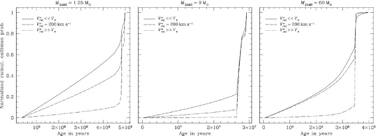
In this work, we only treat collisions between two main-sequence (MS) stars. The motivations for this choice was to keep the number and variety of collisions to consider at a manageable level and that the present version of our Monte Carlo code only includes simplified stellar evolution which skips over the giant phase and turns MS stars directly into remnants. However, in a real stellar system, MS-MS encounters may not dominate the global collision rate. Indeed, a given star of mass $>1\,{{\rm M}_{\odot}}$ may have a smaller probability for colliding with another star during its MS life than during its red giant (RG) phase despite the latter being about 10 times shorter (Bressan et al., 1993, for instance). This is made very clear by integrating the collisional cross-section over the lifetime of the star, as we did in Fig. 2. In many cases, the collision probability during the red giant phase exceeds its MS counterpart for high relative velocities. RG-RG collisions are less likely than RG-MS events. Indeed, the ratio of probabilities can be estimated as follows

$$\frac{P_{\mathrm{RG-MS}}}{P_{\mathrm{RG-RG}}}\sim\frac{n_{\mathrm{MS}}}{n_{\mathrm{RG}}}\cdot\frac{R_{\mathrm{RG}}^{2}}{(2R_{\mathrm{RG}})^{2}}\simeq 0.25\frac{T_{\mathrm{MS}}}{T_{\mathrm{RG}}}\simeq 3-10.$$

Although probably more common than MS-MS encounters, RG-MS collisions may not be more important. RG envelopes have very low densities so only little mass is lost in most cases and the RG recovers its appearance. At relative velocities found in galactic nuclei, the MS star cannot be captured unless it is aimed nearly directly at the RG centre (Bailey & Davies, 1999). Furthermore, as giants will loose their envelope anyway through winds and a planetary nebula or SN phase, collision with giants will probably make little difference as far as the feeding of a central SMBH is concerned.

Due to mass segregation in clusters and nuclei, collisions between compact remnants (CRs) and MS (or RG) stars are probably much more common than the small CR fractional number would suggest. For instance, the innermost 0.1 pc of the Sgr A^∗ cluster is likely dominated by invisible stellar BHs (Miralda-Escudé & Gould, 2000) which may collisionally destroy MS and RG stars. CR-MS and CR-RG collisions may also be of great interest as a way to produce exotic objects, such as cataclysmic variables. Unfortunately, due to the high dynamical range involved, the hydrodynamical simulation of these events is challenging and comprehensive predictions for their outcome are still lacking.

Now that the astrophysical stage is set, we can proceed with a description of our simulation work. In Sec. 2, we describe the choice and setting of initial conditions and present the numerical methods we use to compute and analyse stellar collisions. In Sec 3, results are reported and we explain how to exploit them in stellar dynamical simulations. Finally, in Sec 4, some general conclusions and a discussion of further work to be done are presented.

2 Description of the approach

2.1 Definitions, basic formulae and units

Figure 3: Sketch of a gravitational 2-body hyperbolic encounter in the centre of mass reference frame.

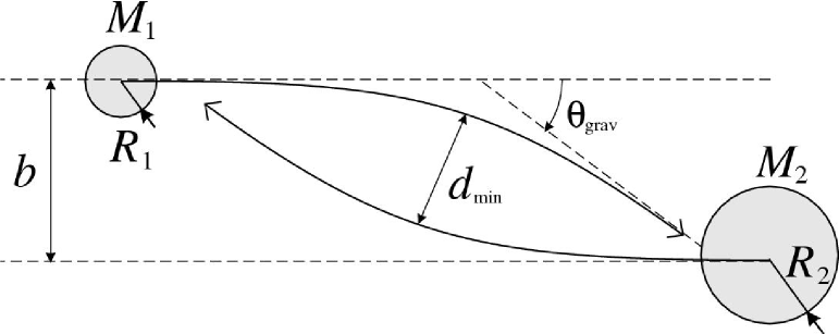
As some quantities will be referred to again and again, we find it useful to define them once for all at the beginning of this article. Collisions between two main sequence (MS) stars are considered. In the centre of mass frame, the collision is completely determined by 4 quantities: the masses $M_{1}$ and $M_{2}$ (in our work, we made the unconventional notation choice: $M_{1}\leq M_{2}$), the impact parameter $b$ (see Fig. 3) and the relative velocity at infinite separation, $V_{\mathrm{rel}}^{\infty}$. The stellar radii are $R_{1}$ and $R_{2}$. Instead of applying a simple but unrealistic power-law mass-radius relation, the values for the radii are taken from the stellar models described in Sec. 2.2.

We shall often refer to the situation of a 2 point-mass hyperbolic encounter where all finite-size (hydrodynamical) effects are neglected. In this case, we define the periastron distance,

$$d_{\mathrm{min}}=(R_{1}+R_{2})\,\frac{2\hat{b}^{2}\hat{v}^{2}}{1+\sqrt{1+4\hat{b}^{2}\hat{v}^{4}}}$$ (4)

with $\hat{b}=b/(R_{1}+R_{2})$ and $\hat{v}=V_{\mathrm{rel}}^{\infty}/V_{\star}$ (see Eq. 6). When gravitational focusing is important, $d_{\mathrm{min}}$ is a more convenient parameter than $b$. Ignoring tidal effects such as deformations and trajectory modification until strong hydrodynamical interactions begin, we assume that only collisions with $d_{\mathrm{min}}<R_{1}+R_{2}$ lead to contact between stars at the first periastron passage.

In case both stars survive the encounter and are left unbound to each other, we define a collisional deflection angle $\theta_{\mathrm{coll}}$. This is the angle between the direction of the initial relative velocity (at infinite separation) with the direction of the final relative velocity (at $\infty$). To assess the importance of finite-size hydrodynamical effects, it is useful to compare $\theta_{\mathrm{coll}}$ with the value for a Keplerian hyperbolic orbit $\theta_{\mathrm{grav}}$,

$$\tan\left(\frac{\theta_{\mathrm{grav}}}{2}\right)=\frac{G(M_{1}+M_{2})}{b(V_{\mathrm{rel}}^{\infty})^{2}}.$$ (5)

A natural velocity scale for collisions is the relative velocity at contact for stars initially at rest at infinity,

$$V_{\star}=\sqrt{\frac{2G(M_{1}+M_{2})}{R_{1}+R_{2}}}.$$ (6)

The structure of MS stars with $M_{\ast}>0.5\,{{\rm M}_{\odot}}$ is very concentrated (see Fig 4 and the appendix) and the total radius is not a good indicator of the extension of the stellar matter. It is thus often useful to normalise quantities with reference to the half-mass radius $R_{\ast}^{\mathrm{(h)}}$, i.e. the radius of a sphere that contains half the stellar mass. These radii can be read from the 50 % curve in Fig. 4. We can then define a “half-mass velocity” scale through

$$V_{\star}^{\mathrm{(h)}}=\sqrt{\frac{2G(M_{1}+M_{2})}{R_{1}^{\mathrm{(h)}}+R_{2}^{\mathrm{(h)}}}}.$$ (7)

This quantity gives a better idea of the relative velocity when strong hydrodynamical effects begin to play an important role. Note that we use total masses in this definition. We often normalise initial parameters by these half-mass quantities so handy definitions are

$$\lambda=\frac{d_{\mathrm{min}}}{R_{1}^{\mathrm{(h)}}+R_{2}^{\mathrm{(h)}}}\mbox{~{}~{}and~{}~{}}\nu=\frac{V_{\mathrm{rel}}^{\infty}}{V_{\star}^{\mathrm{(h)}}}.$$ (8)

Typical scales are set by “solar units”, i.e.:

$${{\rm R}_{\odot}} := 7\times 10^{8}\,\mathrm{m},$$

$${{\rm M}_{\odot}} := 2\times 10^{30}\,\mathrm{kg},$$

$${\rm V}_{\odot} := \left(G{{\rm M}_{\odot}}/{{\rm R}_{\odot}}\right)^{1/2}=436.5\,\mathrm{km\,s}^{-1},$$

$${\rm T}_{\odot} := \left({{\rm R}_{\odot}}^{3}/(G{{\rm M}_{\odot}})\right)^{1/2}=1604\,\mathrm{s}.$$

These values are also referred to as “code units”.

2.2 Stellar models

Figure 4: Mass-Radius relation for the stellar models. The thick line shows the total radius as a function of the mass of the star. Thin lines are for inner Lagrangian radii containing 25 to 95 % of the mass. Data for $M_{\star}\geq 0.4\,{{\rm M}_{\odot}}$ (dots) is from realistic stellar structure models (Schaller et al., 1992; Meynet et al., 1994; Charbonnel et al., 1999). Below $0.4\,{{\rm M}_{\odot}}$, a polytropic ($n=1.5$) structure is applied with a power-law M-R relation extrapolated from higher masses. The run of various Lagrangian radii makes it obvious that stellar models for different stellar masses cannot be deduced from each other through any homologous scaling. The “real” mass, determined through relation 9, is given in abscissa, not the ZAMS value.

In our simulations, we use realistic main sequence (MS) models to set up the initial stellar structures. Models from the Geneva stellar evolution group (Schaller et al., 1992; Meynet et al., 1994) have been applied for ZAMS masses ranging from $0.8$ to $85\,{{\rm M}_{\odot}}$, and models by Charbonnel et al. (1999) for masses down to $0.4\,{{\rm M}_{\odot}}$. For each (initial) stellar mass, we had to select one particular model among those spanning the main sequence evolutionary track. We chose the instant $t_{\mathrm{model}}$ which divides the MS life in two parts with approximately equal collision probabilities. Assuming strong gravitational focusing and neglecting any mass loss, the collision probability per unit time is $\mathrm{d}P_{\mathrm{coll}}/\mathrm{d}t\propto R_{\star}(t)$, so that,

$$\int_{0}^{t_{\mathrm{model}}}\!\!R_{\star}(t)\,\mathrm{d}t\simeq\int_{t_{\mathrm{model}}}^{\min(t_{\mathrm{MS}},12\,\mathrm{Gyr})}R_{\star}(t)\,\mathrm{d}t$$ (9)

with $t=0$ on the ZAMS. For high-mass stars ($\geq 20\,{{\rm M}_{\odot}}$) mass loss by stellar winds is already important on the MS (Schaller et al., 1992; Meynet et al., 1994) so that the adopted models have real masses lower than their nominal (i.e. ZAMS) masses, for instance, the largest star we consider, a “$85\,{{\rm M}_{\odot}}$” model, has an actual mass of only $74.3\,{{\rm M}_{\odot}}$. The mass-radius relation is shown in Fig. 4. For $M\geq 0.4\,{{\rm M}_{\odot}}$, it is given by the stellar models just discussed. For smaller masses, we simply extrapolated a power-law relation from the $0.4\,{{\rm M}_{\odot}}$ and $0.5\,{{\rm M}_{\odot}}$ points. It appears that this gave radii in good agreement with detailed structure models by Chabrier & Baraffe (1997) who yield $R\simeq 0.12\,{{\rm R}_{\odot}}$ at $0.1\,{{\rm M}_{\odot}}$ and $R\simeq 0.22\,{{\rm R}_{\odot}}$ at $0.2\,{{\rm M}_{\odot}}$.

We used models with solar composition ($Y=0.30$, $Z=0.02$). A population II metallicity ($Y=0.24$, $Z=0.001$) would introduce significant alterations in the stellar structures. Most noticeably, low-$Z$ stars are initially more compact, with radii smaller by 10–40 %, and have larger convective cores for $M_{\star}>1\,{{\rm M}_{\odot}}$ (Kippenhahn & Weigert, 1994). For high-mass stars, the most important difference is probably the much weaker mass-loss at lower metallicity (Maeder, 1992). We made no attempt to assess the impact of these effects on collision outcomes. We hope that they can be partially scaled out by a proper dimensionless parameterisation of the initial conditions and results of the collisions (see Sec. 3). While the structure of stars less massive than $0.5\,{\rm M}_{\odot}$ is very close to that of an $n=1.5$ polytrope, more massive evolved MS stars do not match any polytropic model. In particular, stars with $M_{\ast}\geq 1\,{\rm M}_{\odot}$ are more concentrated than $n=3$ polytropes (see appendix for density profiles).

The lowest stellar masses considered are 0.1 and $0.2\,{\rm M}_{\odot}$. For such objects we didn’t use detailed stellar structure models like those by Chabrier & Baraffe (1997) because they rely on a very complex equation of state (EOS) accounting for degeneracy and electrostatic effects. Such an EOS was not available to us for use in the SPH code at the time we embarked on this project. Also, solving this kind of complicated EOS (for each particle at each time step) is done using an iterative scheme and represents a significant computational burden. Instead, we note that the interior of stars with masses lower than $\sim 0.4\,{{\rm M}_{\odot}}$ is nearly completely convective, so their internal structure is very close to that of a $n=1.5$ polytrope (Hansen & Kawaler, 1994; Chabrier & Baraffe, 2000). Given the mass and radius, we can build an initial polytropic star in hydrostatic equilibrium using the EOS for a fully ionised ideal gas. For $0.2\,{\rm M}_{\odot}$, we have compared our simple polytropic model with ideal-gas EOS to a state-of-the-art stellar structure provided by Isabelle Baraffe and found that discrepancies in the density and temperature profiles are below 10 % except for the outermost envelope, a thin layer which is not represented in the SPH structure. Inspecting the realistic $0.2\,{\rm M}_{\odot}$ model, we see that only of order 0.01 % of the stellar mass has temperatures below $10^{5}$ K for which incomplete molecule dissociation and ionisation may be important. Neglecting molecules and partially ionised gas may lead to a slight overestimate of the mass loss because some of the available kinetic energy has to be used to break up molecules and ionise atoms. This is certainly a very small effect as the energy required to completely ionise one gram of stellar matter of solar composition is $1.5\times 10^{6}$ J (Kippenhahn & Weigert, 1994) but the kinetic energy at $500\,\mathrm{km\,s}^{-1}$ (a typical contact velocity for a parabolic collision) is of order 100 times larger.

2.3 The SPH code

Smoothed Particle Hydrodynamics is a Lagrangian particle-based method that has been widely used to tackle all kinds of astrophysical problems, from planetesimal fragmentation to cosmological structure formation. For a description of the method and of its achievements, we refer to reviews by Benz (1990) and Monaghan (1992). See also Steinmetz & Müller (1993) for a critical examination of the pros and cons of the method and Monaghan (1999) for a presentation of its most recent developments.

We used a version of the SPH code that corresponds to the description in Benz (1990). The kernel function is the standard spline introduced by Monaghan & Lattanzio (1985). This code implements a binary tree to compute gravitational forces and find neighbours (Press, 1986; Benz et al., 1990). “Bulk” and von Neumann-Richtmyer artificial viscosity terms are included with $\alpha=2.5$ and $\beta=1.0$.

For the stellar matter, we assume the EOS of a completely ionised mono-atomic ideal gas with account of the radiation pressure:

$$\rho = \frac{\mu}{\mathfrak{R}}\frac{1}{T}\left(P-\frac{a}{3}T^{4}\right)$$ (10)

$$u = \frac{3}{2}\frac{\mathfrak{R}}{\mu}T+\frac{aT^{4}}{\rho},$$ (11)

where $\rho$ is the mass density, $T$ the temperature, $P$ the total pressure, $u$ the specific internal energy, $\mu$ the mean molecular weight, $a=7.56\times 10^{-16}\,\mathrm{J}\,\mathrm{m}^{-3}\mathrm{K}^{-4}$ and $\mathfrak{R}=8314\,\mathrm{J}\,\mathrm{K}^{-1}\mathrm{kg}^{-1}$. The molecular weight of each particle is attributed from the initial stellar structure (see next subsection). It remains constant during the complete SPH simulation. In hydrostatic main sequence stars, the radiation pressure becomes important for masses larger than $5-10\,{{\rm M}_{\odot}}$ (Kippenhahn & Weigert, 1994).

Release of nuclear energy has been shown to have none or very small hydrodynamical influence (Mathis, 1967; Różyczka et al., 1989). We thus do not include nuclear reactions in the energy equation. We also neglect radiative transport. As long as the gas is optically thick (and the bulk of it certainly is during the whole collisional process), energy transport by radiation is a diffusion process which time scale, for a sun-like star is $T_{\mathrm{KH}}\simeq 1.6\times 10^{7}$ years (Kippenhahn & Weigert, 1994, Kelvin-Helmholtz time). This is enormously larger that the hydrodynamical time-scales (a few tens of hours, at most). For a gas cloud of radius $R$ and mass $M$, the diffusion time is:

$$t_{\mathrm{diff}}\simeq\frac{l}{c}N\mbox{~{}~{}with~{}~{}}N=\left(\frac{R}{l}\right)^{2}$$ (12)

where $l$ is the mean free path of photons. It is connected to the opacity $\kappa$ by $l=(\kappa\rho)^{-1}$. Thus,

$$t_{\mathrm{diff}}\approx\frac{\kappa}{c}\frac{M}{R}=120\,{\rm yrs}\times\left(\frac{\kappa}{\kappa_{\mathrm{es}}}\right)\left(\frac{M}{{{\rm M}_{\odot}}}\right)\left(\frac{R}{100\,{{\rm R}_{\odot}}}\right)^{-1},$$ (13)

where $\kappa_{\mathrm{es}}\simeq 0.04\,\mathrm{kg}^{-1}\mathrm{m}^{2}$ is the opacity due to electron scattering (a lower bound for $\kappa$ in ionised gas). It follows that radiation cooling is negligible even long after the end of the collision simulation.

2.4 Building of initial SPH stellar models

Building an SPH star from a given stellar structure model is not completely straightforward. First, the spatial positions of the particles have to be chosen. Then, each particle must be given a mass and smoothing length in such a way that the total mass is respected and the model’s density profile $\rho_{\star}(R)$ is well approximated by the SPH interpolate. A second thermodynamical variable (the internal energy $u(R)$, in our case), as well as the chemical composition, is also specified by the structure model. These quantities determine the pressure through the EOS. If the EOS is similar to the one used in the stellar structure code, the SPH structure should be in hydrostatic equilibrium.

If all particles are attributed the same mass, their number density must closely follow $\rho_{\star}(R)$, which, unless a huge number of particles are used, results in a severe under-sampling of the outer regions where the “action” takes place during most collisions. On the other hand, using a constant particle density throughout the star, by placing them on a periodic grid for instance, will lead to a very inaccurate core representation as a small set of very massive particles. This could expectedly yield unstable initial models and noisy collisional results in case these few heavy particles strongly participate to the hydrodynamics of the encounter. We thus had to find some compromise between these two extreme options. If we neglect particles overlap, the relation $\rho_{\star}(R)\simeq m_{\mathrm{part}}(R)n_{\mathrm{part}}(R)$ holds, with $m_{\mathrm{part}}$ being the local mass of each SPH particle at distance $R$ from the star’s centre and $n_{\mathrm{part}}$ their number density at that position. Thus, we decided to impose

$$n_{\mathrm{part}}\propto\rho_{\star}^{\alpha}\mbox{\ \ and\ \ }m_{\mathrm{part}}\propto\rho_{\star}^{(1-\alpha)}$$ (14)

with $\alpha=0.5$ (the two above mentioned extremes correspond to $\alpha=1$ and $\alpha=0$ respectively). To obtain a $R$-dependent $m_{\mathrm{part}}$, we place particles on concentric spheres with variable spacing. On each sphere particles are arranged on constant “latitude” circles. When this is done, the smoothing lengths $h_{i}$ are adjusted until each particle overlaps approximately with the same number ($\simeq 40$) of neighbours’ centres. Finally, particles’ masses are iteratively adjusted in order to bring the SPH interpolate for the density (at the centre of particles) closer to the model’s $\rho_{\star}$. This is done by repeating the assignments

$$m_{i}\leftarrow m_{i}\left(0.3+0.7\frac{\rho_{\star}(R_{i})}{\rho_{i}}\right)\ \ i=1\ldots N_{\rm part}$$

20 times. As this procedure doesn’t conserve the total mass $M_{\ast}$ exactly, all $m_{i}$ are then slightly rescaled by a uniform factor to obtain the required $M_{\ast}$. This method is fast and effective to give a good match to $\rho_{\star}$ for the bulk of the stellar interior, as testified by the profiles shown in the appendix. But, despite the use of lighter particles to represent the gas in the stellar envelope, the outermost layers of the star are poorly modelled. In particular the SPH realisation fails at precisely reproducing the stellar radius. This had to be expected in models with a limited number of particles.

Nonetheless, in grazing collisions, our use of low-mass SPH particles to represent the outer parts of a star apparently leads to a reliable determination of fractional mass losses as small as $10^{-4}$–$10^{-3}$. This claim is grounded on diagrams like Fig. 5 which shows the fractional mass loss for two sets of simulations, the first one with the “normal” (low) resolution and the second one with a number of particles about four times larger. The differences are obviously very small for all cases but the most distant interactions.

Figure 5: Fractional losses of mass (top panel) and energy (bottom) as functions of the distance of closest approach (in Keplerian approximation) for fixed $(M_{1},M_{2},V_{\mathrm{rel}}^{\infty})$. Three sets of simulations are reported. In the first one (solid lines) we use a relatively low number of SPH particles and our standard (rather large) value for the binary tree accuracy parameter acc (Benz et al., 1990). In the second series, we used about four times more particles. In the third, we used a lower acc value which gives a more precise computation of gravitational forces. The results are nearly coincident. $T_{\mathrm{cont}}$ is the kinetic energy at contact, i.e. for a separation between centres of $R_{1}+R_{2}$.

An extended coverage of the four dimensional $(M_{1},M_{2},V_{\mathrm{rel}},b)$ parameter space requires a huge number of collisions to be computed. On the other hand, we don’t need very accurate results; a relative precision of about 10 % on mass and energy loss should be sufficient for our purposes. More precise results would not make much sense anyway as any application will probably require some sort of inter- or extrapolation from our simulation data, to apply it to stars with different masses or metallicities, for instance. Thus we decided to tune numerical parameters to values that allow relatively fast computations while ensuring reasonable accuracy. This means that we generally used 1000–8000 SPH particles for each stellar model (a few collisions have been computed with the most massive star having $\sim$16 000 or $\sim$32 000 particles). In most simulations the total number of particles ranges between 2000 and 10 000. Thus, a collision is computed in a few hours to a few days on a run-of-the-mill workstation. We use a higher number of particles in high mass stars in an attempt to resolve both the high density centre that contains most of the mass and the low density envelope which is more likely to interact with the other star. We also adapt the number of particles of both stars in order to get spatial and mass resolution not too dissimilar for stars of unequal sizes. As an example, for equal mass stars we generally use 2000$+$2000 particles for low masses ($\leq 1\,{\rm M}_{\odot}$) and 4000$+$4000 particles for high masses. These numbers are certainly not impressive by present-day standards but already corresponded to considerable computational burden given the large number of collision to simulate and the typical speed of computers at the time this study was initiated, more than five years ago. We now discuss the test computations we made to ensure these particle numbers were sufficient for our aims.

2.5 Determination of the required resolution

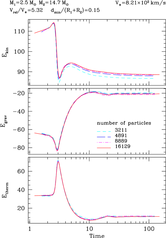
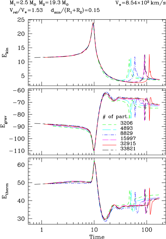
To determine the minimal desirable number of particles to be used in our simulations, we computed the same physical collision with various $N_{\mathrm{part}}$. Fig. 6 shows the evolution of the energies during two typical collisions simulated with increasing numbers of particles. In all these cases but one, the number of particles in the small star is $\sim$1000 while the large star consist of $\sim$2000 to $\sim$32 000 particles. The first collision is a high-velocity quasi-hyperbolic “fly-by”. In the second example, the stars are left bound to each other after the first periastron passage. A second collision ensues that leads to a rapid merging of the small star into the centre of the big one. In the “fly-by” case, the energy evolution curves for the various $N_{\mathrm{part}}$ values are very similar to each other as soon as more than 2000 particles are used to represent the large star. Contrariwise, in the “merger” case, the time between the two successive periastron passages exhibits a strong dependency on $N_{\mathrm{part}}$. Not only does it not converge to some “real” value as the resolution is increased but the opposite occurs! This intriguing behaviour casts important doubts on the ability of this version of the SPH code to follow reliably the formation and evolution of tidal binaries. However we note that a simulation with $32000+2000$ particles (the last one in the right panel of Fig 6) gives nearly exactly the same energy evolution as another one with $16000+1000$ particles (the fourth one). This is a hint at the importance of a good resolution in both stars and not only the larger. Convergence in the results is attained only if we increase both resolutions. It is not clear to us why this is so but it is obviously connected to the poorly resolved envelope structure which determines how much orbital energy is dissipated at first passage. This turns out to have very little implication for the amount of mass loss, the only quantity we want to determine in case of a merger. As shown on Fig. 5, it is only for grazing fly-bys that one get significant relative discrepancy between different resolutions, as long as energy and mass loss are concerned. This also is due to inaccuracies in the SPH realisation of the outer layers. But given the very small absolute values of these losses, this can only have very small impact when SPH results are used to implement collisional effects in simulations of high-velocity stellar systems.

In any case, in our work, we are mostly interested in the final outcome of collisions in terms of global quantities, like the mass and energy loss. The dependency of these quantities on $N_{\mathrm{part}}$ turns out to be very weak. The fractional mass and energy losses and the fractional deviation from the Keplerian deflection angle typically vary by less than 20 % over the whole range of particle numbers used in these tests (see appendix for diagrams). While the lowest $N_{\mathrm{part}}$ produce results that are somewhat off, as compared to higher resolution runs, 1000$+$2000 particles seem to be already sufficient.

Figure 6: Evolution of the system energies during two collisions. Each collision has been computed with different resolutions (3000 to 34 000 particles). Code units are used here. The quantities describing the collisions are specified on top of the diagrams. See text for further comments. The left column is a “fly-by” encounter. The right column corresponds to a merger (see Fig. 7).

2.6 Starting, ending and analysis of a collision simulation

Any collision to be computed requires the specification of both stellar models and of the relative velocity at infinity $V_{\mathrm{rel}}^{\infty}$ and the impact parameter $b$. We neglect any finite-size effect until the separation between the stars’ centres is $3(R_{1}+R_{2})$. Hence we analytically advance the stars to this situation on hyperbolic trajectories. At this point, we start the SPH simulation and set $t=0$.

The computation stops at $t_{\mathrm{end}}\geq 20\,T_{\mathrm{dyn}}$ with $T_{\mathrm{dyn}}=\sqrt{(R_{1}+R_{2})^{3}/(G(M_{1}+M_{2}))}$. If, at this time, two surviving stars are present with separation less than $3(R_{1}+R_{2})_{\mathrm{ini}}$ or if the amount of gas with uncertain fate (see next paragraph) exceeds 1 % of the total mass, the simulation is integrated further (by setting $t_{\mathrm{end}}\leftarrow 2t_{\mathrm{end}}$) until it passes these tests or some maximal integration time is reached. In practise, no collision required integration past $t=2500\sqrt{{{\rm R}_{\odot}}^{3}/(G{{\rm M}_{\odot}})}$. Unfortunately, these simple termination prescriptions are probably inadequate when a bound binary forms after first periastron passage. They can indeed force integration for many orbital periods although we expect the SPH scheme (at least when used with our set of numerical parameters) to lose reliability in that regime whose outcome is very likely to be a merger (see Sec. 3.1). A wiser approach would have been to identify such encounters, stop computation after first passage at periastron and, if needed, to rely on other theoretical considerations to assess the outcome.

One monitors the energy (non-)conservation with $\delta_{E}=\left|E_{\rm end}-E_{\rm ini}\right|/E_{\rm norm}$ with $E_{\rm norm}=E_{\rm kin}^{\infty}+E_{\rm bind}$, where $E_{\rm ini}$, $E_{\rm end}$ are the initial and final total energies, $E_{\rm kin}^{\infty}$ the initial kinetic energy at infinity (orbital energy) and $E_{\rm bind}$ the sum of the binding energies of the stars (positive definite). Using the total energy, $E_{\rm ini}=E_{\rm kin}^{\infty}-E_{\rm bind}$ for normalisation isn’t appropriate because it may be very close to zero, leading to misleadingly large values of $\delta_{E}$. $E_{\rm norm}$ gives a natural energy scale for the problem. Using $E_{\rm bind}$ for normalisation doesn’t change much the $\delta_{E}$ statistics. The worst non-conservation amongst all simulations is $\delta_{E}\simeq 0.06$; all but 15 simulations have $\delta_{E}<0.01$; 66 % of all runs have $\delta_{E}<0.001$.

The SPH code yields quantities describing every particle at the end of the computation, i.e. their positions, velocities, internal energies…This raw “microscopic” data has to be analysed to provide a useful description of the outcome of the collision in terms of “macroscopic” quantities, i.e. properties of outgoing star(s) (if any). Namely, we want to know how many stars survive (0, 1 or 2) and what their masses, positions and velocities at the end of the computation are. This, and any other aspect of the structure of the star(s) (see Sec. 3.3) and of the ejected gas, can be easily determined if we manage to build a list stating to which star each particle belongs or whether it is unbound to any surviving star. This data is provided by an analysis algorithm which proceeds in two steps:

1. A first guess attribution is realised by a code which tries to identify, through density and proximity criteria, zero, one or two concentrated lumps of particles. To this end, we use the freely available HOP algorithm by Eisenstein & Hut (1998). These groups are regarded as first approximations of stars to be refined in the second stage of the method.

2. We then iteratively cycle through all particles to compute the energies of each one relative to both stars (“A” and “B”). For iteration $k$, the energy of particle $i$ relative to star A as identified at the previous iteration (“A_k-1”) reads

   $$\left.E^{\mathrm{A}}_{i}\right|_{k} = u_{i}+\frac{1}{2}m_{i}\left(\vec{v}_{i}-\vec{V}_{\mathrm{A}_{k-1}}\right)^{2}$$ (15)

   $$-Gm_{i}\!\sum_{j\in\mathrm{A}_{k-1}}\!\frac{m_{j}}{\left\|\vec{x}_{i}-\vec{x}_{j}\right\|}.$$

   In this formula, $u_{i}$, $m_{i}$, $\vec{v}_{i}$ and $\vec{x}_{i}$ are the internal (thermal) energy, mass, velocity and position of particle $i$. $\vec{V}_{\mathrm{A}_{k-1}}$ is the velocity of “star” A_k-1, i.e.

   $$\vec{V}_{\mathrm{A}_{k-1}}=\sum_{\mathrm{A}_{k-1}}\!m_{j}\vec{v}_{j}\left/\sum_{\mathrm{A}_{k-1}}\!m_{j}\right..$$

   If either $\left.E^{\mathrm{A}}_{i}\right|_{k}$ or $\left.E^{\mathrm{B}}_{i}\right|_{k}$ is negative, the particle is ascribed to the “star” relative to which its energy is the most negative. Particles with positive energies relative to both stars but with negative total energy in the collision centre-of-mass reference frame (CMRF) are tagged as “doubtful”. At the end of the iteration we thus get new sets of particles making up “stars” A_k and B_k. We go on iterating until no modification in the composition of these sets occurs anymore.

This procedure deserves a few comments.

• The energy criterion may fail to predict the correct attributions. For instance, a particle with high velocity toward a given star may happen to have positive energy relative to this star even if it will impact it and thus merge into it. Furthermore, even without resorting to hydrodynamical processes, we learn from studies of the gravitational 3-body problem that the eventual fate of a particle submitted to the gravitational forces of two massive bodies can not generally be predicted just through energy consideration. However, if we carry on the SPH integration to a physical time large enough for the stars to have moved away from each other to a large separation and/or for the large amplitude hydrodynamical processes to have ceased, we expect the final SPH configuration to be essentially free of such problematical particles and the energy criterion to be reliable.

• “Doubtful” particles generally lie between the two stars so that they gain negative gravitational contributions to their total energy from both potential wells even though they are not bound to any one star. In such cases, their number should decrease as the distance between the stars increases. Another situation that can leave a relatively important doubtful mass fraction (i.e. $>1$ % of the total mass) occur in high velocity head-on collisions that result in an expending gas cloud. Its central part, lying in the potential well of the surrounding gas has negative total energy but nevertheless expands to infinity. Although these cases seem to have genuine physically interpretations, there are situations where a high $M_{\mathrm{doubt}}$ is indicative of some error in the analysis. One such case consist of a close tidal binary being erroneously identified as a single particle group in the first step. The iterative steps then progressively interpret one of the stars as a group of doubtful particles while retaining only the other lump as a “real” star.

• This last example illustrates how critical the first attribution stage is. Its failure to detect independent stars cannot be recovered by the iterative process! There is probably room for improvement in this part of our analysis procedure and the use of HOP, an algorithm aimed at finding structures in large cosmological simulations, is arguably an inefficient overkill. A simple-minded approach that first divides particles in the same two groups that built up the pre-encounter stars proves to allow convergence to real stars in cases that confuse HOP. To account for mergers, when the distance between the centres of the two groups is much smaller than some typical size, we can ascribe all particles to a single group to be then “eroded” down to the bound star (if it exists) by the iterative energy test.

All simulations were first analysed using HOP to produce the initial particle attributions. The results of the iterative procedure were then visually inspected by plotting $\log\rho$ versus spatial coordinate $x$ for all SPH particles and using different colours to code the attributions. Errors are immediately spotted in such a diagram allowing one to integrate the simulation for a longer time if the separation between “stars” (density peaks) is deemed too small or switching to the just-mentioned simple-minded scheme for initial attributions in the few cases HOP clearly made a wrong guess.

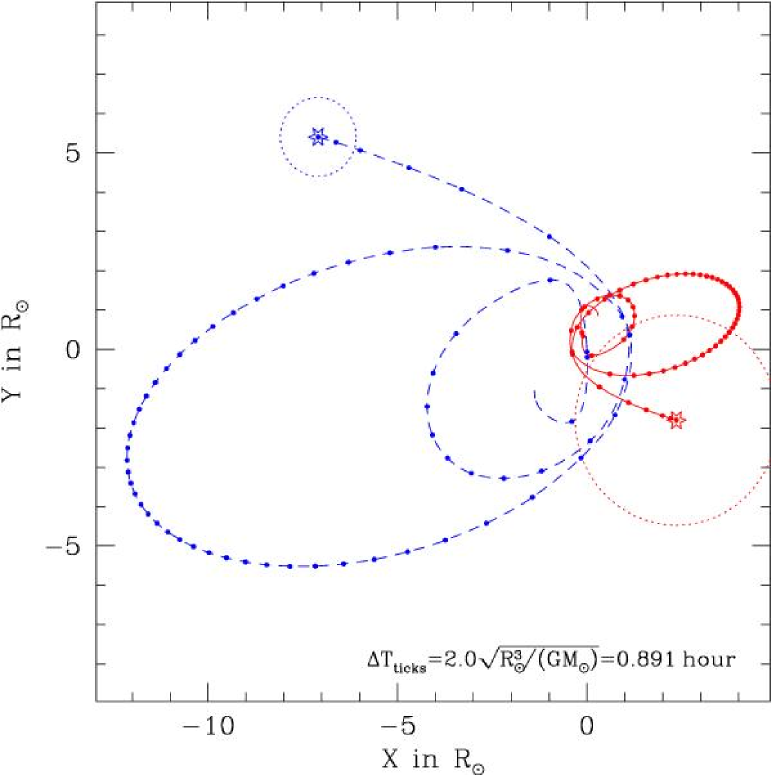
In the vast majority of simulations, we only run the analysis software just described on the final SPH file. As mentioned above, if, for that configuration, $M_{\mathrm{doubt}}$ exceeds some fraction of the total mass (1 %) or wrong attribution is seen, we compute the interaction for a longer physical time. When the integration is deemed over and the properties and kinematics of the surviving star(s) have been determined, we assume that the stars’ masses have reached constant values and that the subsequent orbital evolution is purely Keplerian again. This allows to compute $\theta_{\mathrm{coll}}$ as an asymptotic value. The physical time $t_{\mathrm{end}}$ over which the SPH simulation is computed has thus to be long enough for the strong hydrodynamical regime to be over. On the other hand, choosing too large a value for $t_{\mathrm{end}}$, is not only computationally expensive but could result in inaccurate results due to the accumulation of small numerical errors. Hence, it is of interest to analyse a few typical collisions at a number of increasing times during the SPH computation to test whether the outcome quantities have reached steady values and whether these values show sign of numerical drift at large $t$. Fig. 7 is an example of such computations. The plot of the trajectories (panel (a)) testifies that, in most cases, the analysis procedure identifies the stars correctly, even during close interaction. The curves for the evolution of predicted mass and energy losses show abrupt increases at periastron passages and stay nearly constant quickly after the last close encounter (leading to a merger) is over. Although the analyse software gets confused when the stars penetrate each other, this is of no practical concern because it is only a transitory situation. For fly-bys (including the case the small star emerges as an unbound, expanding cloud), we integrate until the stars are again very well separated; when stars capture each other, the analysis is only done after a merged object has formed or when the stars, forming a binary, do not overlap. We conclude that the way we terminate SPH collisions and analyse their results is sound.

(a)	(b)

Figure 7: Collision between stars with $M_{1}=1\,{{\rm M}_{\odot}}$, $M_{2}=3\,{{\rm M}_{\odot}}$, $V_{\mathrm{rel}}^{\infty}=0.07V_{\ast}=43.7\,\mathrm{km}\,\mathrm{s}^{-1}$, $d_{\mathrm{min}}/(R_{1}+R_{2})=0.39$. Panel (a): Trajectories of colliding stars, as identified by the algorithm used to analyse the outcome of collisions. This encounter leads to the formation of a binary which coalesce after two orbits. The analysis algorithm is unable to tell one star from the other during the final merging. Panel (b), top: Evolution of the separation between both stars. Panel (b), bottom: Evolution of the amount of gas unbound to any star, with positive or negative energy in the centre-of-mass reference frame ($\delta M_{\mathrm{loss}}$ and $\delta M_{\mathrm{doubt}}$ respectively). This diagram illustrates how the mass loss increases abruptly at each periastron passage and reaches a steady value after complete merging. The amount of gas with doubtful fate also gets quickly to a vanishingly small value. This ensures that the interaction has been integrated for a sufficiently long time.

2.7 Building a comprehensive table of collisions

Figure 8: Diagram depicting the initial conditions for all the collision simulations we performed. Dots in each small box represent the pericentre distance $d_{\rm min}$ (in units of the stellar radii) and relative velocity at infinity $V_{\rm rel}^{\infty}$ (in units of $V_{\odot}=436.5\,\mathrm{km\,s}^{-1}$) of all simulations for a given $(M_{1},\,M_{2})$ pair. The enlarged box displays the $(d_{\rm min},\,V_{\rm rel}^{\infty})$ plotting area. Note that the masses axis are neither linear nor logarithmic but simply represents the differents masses in a sequence.

This study was first embarked on as a sub-project. It is part of a work aimed at simulating the stellar dynamical evolution of dense galactic nuclei hosting black holes. To this end, a new Monte Carlo code for cluster dynamics has been developed (Freitag & Benz, 2001b, 2002). In order to incorporate the effects of stellar collisions with a high level of realism into it, we decided to compute a large number of SPH simulations spanning all the relevant values of the initial conditions. Our hope was then to extract fitting formulae from this database of results to get an efficient description of the outcome of any arbitrary collision that could occur during a cluster simulation run. Figuring out such mathematical descriptions proved too difficult and we have resorted to an interpolation procedure. This will be explained in Sec. 3.3.

Contrary to globular clusters where all collisions are essentially parabolic due to the velocity dispersion being much lower than the escape velocity from a stellar surface, galactic nuclei may have deep potential wells, or even harbour massive black holes and thus force some of their inhabiting stars to collide on high-velocity hyperbolic trajectories. For instance, at the centre of the Milky Way, “SO” stars are on orbits with pericentre velocities of up to $\sim 12\,000\,\mathrm{km\,s}^{-1}$ (Ghez et al., 2005; Schödel et al., 2003) and even higher values will probably show up in future higher resolution observations reaching closer to the $\sim 3-4\times 10^{6}\,{{\rm M}_{\odot}}$ black hole Sgr A^∗. Hence, we cannot restrict ourselves to collisions with $V_{\mathrm{rel}}^{\infty}\simeq 0$ but have to go up to a few thousands of $\mathrm{km\,s}^{-1}$.

Moreover, the population in galactic nuclei does not consist of old stars all born at the same time but may include MS stars with an extended range of masses. High mass stars are particularly important in the first phases of the system evolution: relaxation-induced mass segregation may quickly concentrate them in the high density central regions where, having large cross sections, they get relatively high collision probabilities, despite their overall scarcity and their short MS lifetimes. Consequently, we have also to span a large range of initial masses, extending far beyond the $\sim 1\,{{\rm M}_{\odot}}$ tun-off mass that would be sufficient for a study of collisions in present-day Galactic globular clusters.

Finally, to further extend the domain in parameter space to be explored, we note that stars of different masses have very different internal structures (see density profiles in appendix) so we cannot hope to scale out the absolute mass from the collision process. For instance, we would expect the (dimensionless) results to depend only on the mass ratio $M_{1}/M_{2}$ only if stellar structures were homologous to each other and a power-law $M$–$R$ relation was obeyed. As this is not true, we have to consider the masses of the in-coming stars as two independent variables.

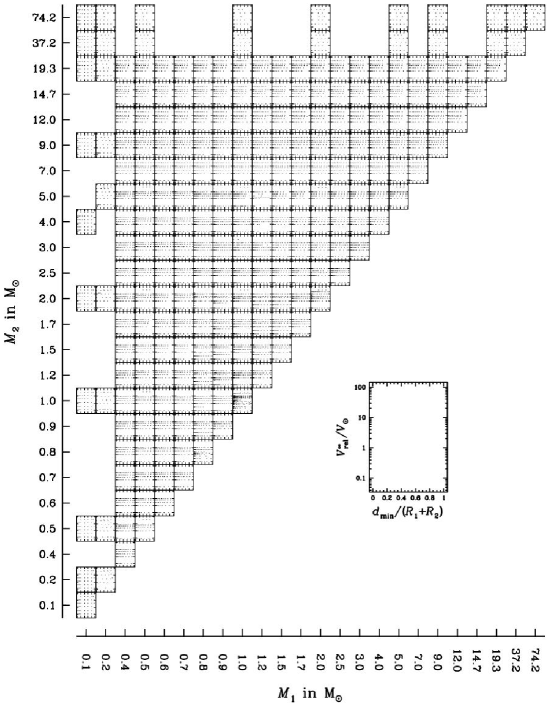
Summing it up, we have to deal with a fully 4-dimensional parameter space in which we have sampled a domain which is more or less the following:

• Stellar masses from 0.1 to 74.3 ${{\rm M}_{\odot}}$ (the latter value corresponds to a ZAMS mass of 85 ${{\rm M}_{\odot}}$).

• Relative velocities in the range $V_{\mathrm{rel}}^{\infty}/V_{\ast}\simeq 0.03$–$30$.

• Impact parameters corresponding to $d_{\mathrm{min}}/(R_{1}+R_{2})=0$–$0.9$.

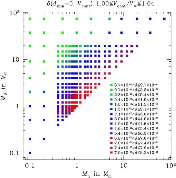
A mere 10 points resolution for each parameter already turns to a total of 10 000 collisions to be computed, a number clearly beyond what can be managed “by hand”. This high number grounded our decision to neglect other, “second order”parameters such as metallicity, rotation or evolutionary stage along the MS track. A complete software system, consisting of many UNIX shell scripts has been developed to run these SPH simulation in a (nearly) completely automatic way. The system looks through a table for collision simulations that have not yet been computed to their end and makes them run on idle workstations available through the local computer network. The system interrupts a simulation job when the computer on which it’s running ceases to be “available” (basically during daytime) and calls the analysis software when a run is over. If no further integration is required, the results are added to an output table. Supervising this automatic system is not as painless as it may sound: due to the number of simulations that run concurrently (10 to 50, typically), “exceptional” problems mainly originating from malfunctions in the local network occur nearly every day and have to be fixed manually. All in all, obtaining a system reasonably crash-proof revealed itself to be unexpectedly difficult. This paper reports on the results of the $\sim$14 000 simulations we managed to compute with this approach. On Fig. 8, we attempt to show the initial conditions for all simulations.

2.8 Formation of binaries through tidal interactions

Even when the periastron distance is larger than the sum of the stellar radii, close encounters at low relative velocity can rise tides in the interacting stars and lead to the formation of a bound binary. As already pointed out by Fabian et al. (1975), in globular clusters, the cross section for such tidal captures is a factor 1–2 times as large as for collisions (assuming a typical relative velocity of 10 $\mathrm{km\,s}^{-1}$). Determining through SPH simulations the critical impact parameter for tidal captures in (quasi-)parabolic, non-touching encounters is a demanding task, requiring high resolution of the stellar envelopes where tides transfer energy from the orbital motion to stellar oscillations. This phenomenon is not treated in this paper because, in typical galactic nuclei, the relative velocities are in excess of 50 $\mathrm{km\,s}^{-1}$, a regime where tidal binaries can form only for very close encounters, requiring contact interaction in most cases, with the possible exception of less concentrated, low-mass stars (Lee & Nelson, 1988; Kim & Lee, 1999). Hence, we restricted ourselves to the range $d_{\mathrm{min}}<(R_{1}+R_{2})$.

3 Results

3.1 Overall survey of the results

Trying to get a complete coverage of collision parameter space implies a huge volume of simulation results. The difficulty of our approach is to extract useful information in manageable form out of these data. As the database was nearing completion, we looked for mathematical relations between various input and output quantities. Due to the deterministic nature of collisions, many strong correlations are clearly visible but finding fitting formulae for them eluded us. The basic difficulty stems from dimensionality of the initial parameter space which seems to be genuinely 4D.

Here we do not show the results from specific collision simulations nor discuss the physical mechanism at play during them, as this has been done extensively in previous works (Benz & Hills, 1987, 1992; Lai et al., 1993; Lombardi et al., 1996). For the interested reader a few specific simulations are presented in the appendix. What concerns us here is a description of the simulation database as a whole.

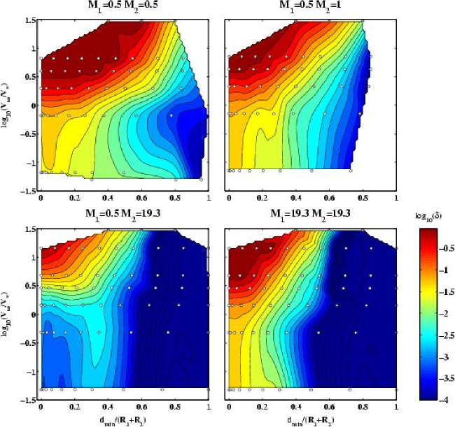
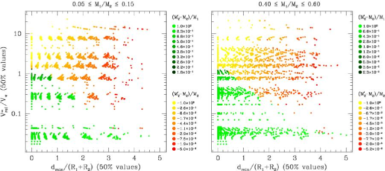
The simplest, most qualitative, description of the collisional outcome is the number of outgoing star(s). For given initial masses, we can plot a 2D diagram indicating this number for all collision simulations performed, as a function of the impact parameter and the relative velocity (Fig. 9).

Figure 9: Number of stars surviving collisions. Red dots are for collisions leading to complete disruption, blue dots for cases with one surviving star, orange dots for tidal binaries (very likely to eventually merge) and green dots for encounters with two surviving stars. See text for further explanations and comments.

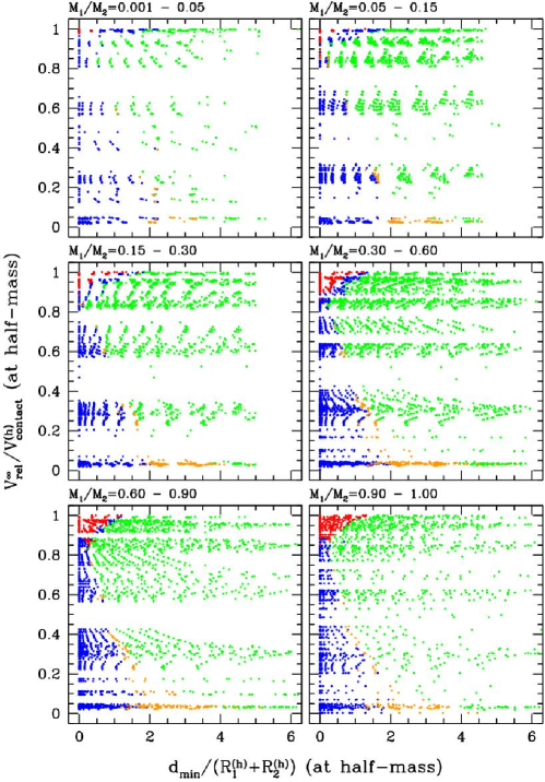
Before we comment on that figure, some explanations are called for. $V_{\mathrm{contact}}^{(\mathrm{h})}$ is an approximate value of the relative velocity at “half-mass contact”. It is defined through

$$V_{\mathrm{contact}}^{(\mathrm{h})}=\sqrt{\left(V_{\mathrm{rel}}^{\infty}\right)^{2}+\left(V_{\ast}^{(\mathrm{h})}\right)^{2}}.$$ (16)

It should be noticed that such a “deep” contact does not occur during encounter with large impact parameters; this value only serves as a convenient parameterisation that allows to map the $[0,\infty[$ $V_{\mathrm{rel}}^{\infty}$ range onto $[0,1[$. In these plots, each dot represent one SPH simulation. Green dots are collisions survived by both stars (although significant amount of mass loss may have occurred). Blue dots indicate that there is only one star left at the end of the encounter. Orange dots stand for tidal binaries and red dots for complete disruption of both stars. One sees that, for this half-mass parametrisation of the initial conditions, the borders between these various regimes are primarily set by the mass ration $q=M_{1}/M_{2}$, quite independently of the actual masses. Unfortunately, as will be stressed below, this appears generally not to hold for more quantitative results.

These diagrams provide a division of the collisions into a few different regimes. Most of the $(d_{\mathrm{min}},V_{\mathrm{rel}})$ plane is occupied by “fly-bys”, i.e. encounters from which two unbound stars escape. In some cases, this domain extends to $d_{\mathrm{min}}=0$ like a small wedge between the merger regime (lower velocities) and disruptions (higher velocities). It is thus possible for a small star to pass right through the centre of a larger one and not being disrupted. We detected about 250 such cases in our survey, all with $q$ between 0.04 and 0.25 and $M_{1}$ (small star) between 0.7 and $2\,{{\rm M}_{\odot}}$. Moreover, in about one third of these simulations (with $\nu<1.7$), the small star gains mass during the interaction while the larger star always suffers from important mass loss. It seems even possible that in some collisions, the small star, acting like a bullet, shatters its target but remains nearly intact. Similar outcomes were obtained by BH92 for $n=1.5$ polytropes with $q=0.2$. LRS93 did not find any head-on collision with a surviving small star. As pointed out by these author, such discrepancies –as well as other differences between our results and published data, see Sec. 3.2– probably originate in the fact that different stellar models have been used. The ratio of stellar central densities is likely to be a key parameter in allowing such “fly-through” collisions. In all the cases identified by us, this ratio exceeds 6. However, the astrophysical importance of this phenomenon is low because, at large relative velocities, collisions with small $d_{\mathrm{min}}$ are unlikely as gravitational focusing is quenched.

Mergers or bound binaries are formed during encounters with low relative velocities and impact parameter below some critical $\lambda_{\rm merg}$. This value depends on the relative velocity and the masses (mostly through the mass ratio). It is apparent as the transition between green and orange or blue dots on Fig. 9. It is generally larger than $R_{1}^{({\rm h})}+R_{2}^{({\rm h})}$ for $\nu<0.6$ and smaller at larger velocities. An ad-hoc analytical parametrisation of $\lambda_{\rm merg}$ as a function of $M_{1}$, $M_{2}$ and $\nu$ will be published soon (Freitag et al., 2005b). Remarkably, the maximum velocity for a head-on collision that still leads to merger is $\nu\simeq 1.7-2.1$, quite independently of the stellar models. The border between this region and the “fly-by” regime at higher $d_{\mathrm{min}}$ is also rather well defined if half-mass variables are used.

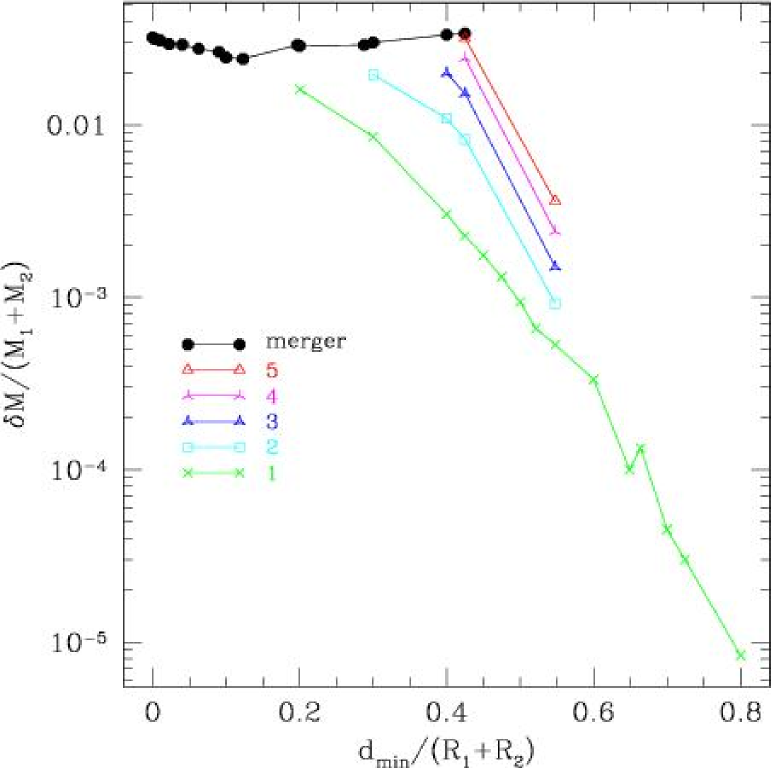
All binaries formed in our simulations will presumably merge into single stars after a few orbits. The reason for this is that, at each periastron passage with $d_{\mathrm{min}}<(R_{1}+R_{2})$, some orbital energy is converted into heat by shocks and the stellar radii expand so that at next periastron passage the hydrodynamical interaction is stronger and more energy is dissipated (Benz et al., 1989). Hence, the fate of these binaries is not as complex an issue as the long-term orbital evolution of systems formed through more distant encounters (Mardling, 1995a, b). Thus, the border between the regions of merging and binary formation probably results from the criteria we use to stop the SPH computations and has no strong physical meaning. If it were possible to integrate the evolution for many orbital periods, there is little doubt that any binary would eventually merge. Fig. 10 illustrates this point. To produce this diagram we computed a set of collisions with increasing $d_{\mathrm{min}}$ for given stellar models and a fixed value of $V_{\mathrm{rel}}^{\infty}$ which is sufficiently low that every collision leads either to direct merger or binary formation. Unlike the bulk of our simulations for which we analysed only the “final” state, here we report the mass loss after each successive periastron passage. Obviously, as $d_{\mathrm{min}}$ is increased, the number of orbits preceding the final coalescence get higher and higher, as does the orbital period. Consequently, the required CPU time grows up to unacceptable values. A noticeable feature of Fig. 10 is that all the collisions apparently converge to nearly the same total mass loss at merging. The reason for this behaviour is unknown to us.

Figure 10: Fractional mass loss for collisions between stars of masses $1$ and $5\,{{\rm M}_{\odot}}$ with a relative velocity at infinity of $43.7$ km s^-1. We indicate the mass loss for each successive periastron passage. The line with crosses (green in the colour on-line version) shows the mass loss after the first passage, the line with open squares (cyan) the mass loss after the second passage and so on until the stars have merged. The total mass loss is shown by the line with round dots (black). For the most central collisions ($d_{\mathrm{min}}<0.425$), the evolution was integrated up to final merging. This was not possible for more distant encounter due to the important increase in computing time this would require and the loss of numerical precision to be expected in such long SPH integrations.

Apart from the low velocity merging zone, another region with one surviving star is present in the diagrams of Fig. 9. This second zone is more or less confined between cases where stars are completely destroyed (for lower impact parameters) or both survive (for higher impact parameter). This “one-star band”, which does not show up when the two stars are (nearly) identical, is populated by collisions during which the small impactor is disrupted without being accreted into the large star. In such high velocity collisions, the small star accumulates so much thermal energy as it flies through the massive one, that it turns into an unbound, expanding gas cloud.

The most spectacular collisions are those that lead to complete disruption of both stars. However, to achieve this result, we note that both a high relative velocity and a small impact parameter are required, a combination made unlikely by the absence of gravitational focusing at such high velocities so it is clear that neither mergers nor complete disruptions are likely outcome in galactic nuclei, as confirmed by Monte Carlo simulations (Freitag & Benz, 2002; Freitag et al., 2004a).

3.2 Comparison with literature

Figure 11: Collisional fractional mass loss. We compare some of our simulations (dots and solid line spline interpolation) with results from the literature (see text). To obtain the “Spitzer & Saslaw 66” (SS66) curves we applied the method of these authors to our stellar models. Panels (a) and (b): for such small mass stars, the structure is quasi-identical to a $n=1.5$ polytrope. This is why we get a good agreement with BH87 and BH92 but big discrepancies with formulae from LRS93 and R99, as these authors use more concentrated $n=3$ structures. Note that the SS66 prescription gives very satisfying prediction for off-axis encounters! Panel (b) This is a case with relatively good agreement with published formulae. Still, the predictions from R99 and LSR93 are 2–3 times larger than our mass losses. The agreement with SS66 is excellent as soon as $d_{\mathrm{min}}/(R_{1}+R_{2})>0.15$. Panel (d): Here, the best agreement is obtain with the R99 formula, despite the velocity being a bit lower than the range explored for this work. SS66 gives satisfactory results, but not LRS93. The reason for this discrepancy is unknown. See caption of Fig. 14 for the probable explanation of the bump at $d_{\mathrm{min}}/(R_{1}+R_{2})\simeq 0.2$ in our curve.

Figure 12: Similar to Fig. 11. Here we push results from the literature somewhat beyond their natural range to test for their predictive power. Panel (a): the poor agreement between us and R99 and LRS93 is due to $0.5\,{{\rm M}_{\odot}}$ MS stars being much less concentrated than $n=3$ polytropes. Panel (b): the disagreement with R99 originates in the low velocity we use. The same may be true for LRS93. Note that our result for large impact parameter is probably an under-estimate. For such low initial velocities, we expect the formation of a binary and a subsequent merging to occur. However, it is likely that we did not integrate past the first pericentre passage (see Fig.10). The flatness of the curve of LRS93 may reflect this phenomenon. Panel (c): here, we have smaller mass ratio than any simulations from LRS93 and R99. The agreement with R99 at large $d_{\mathrm{min}}$ is probably fortuitous. Panel (d) The discrepancy with BH87 stems from our use of completely different stellar models. R99 provides not so bad an agreement, given the low value of velocity. The mismatch with LSR93 is of more mysterious nature. This is one of the few cases where SS66 prescription fails at large impact parameters.

Figure 13: Similar to Figures 11 and 12. In these diagrams, we make comparisons with individual simulation results from LRS93 (crosses, from their Fig. 13). In the legends for the LRS93 data, $q$ is the mass ratio, $\alpha_{1}$ ($=\alpha_{>}$ in our text) the $\alpha$ value (see text) of the more massive star (beware that, contrary to us, LRS93 use “1” to designate the the massive star), $v_{\infty}=V_{\rm rel}^{\infty}(GM_{>}/R_{>})^{-1/2}$ where $M_{>}$, $R_{>}$ are the mass and radius of the massive star. Note that, when applying LRS93’s formulae for the mass loss (long dashes), we determine $\beta_{>}$ (equivalent to $\alpha_{>}$, see text) for our stellar models, through the relation $\beta\simeq 2E/W$ where $E$ is the total energy of the star (thermal plus gravitational) and $W$ its gravitational energy. In general, this corresponds to a value of $\alpha$ different from the one used in the LRS93 simulations. This explains the possible mismatch between the long-dashed line and the crosses.

In this section, we perform critical comparisons between our results and data and methods previously published (see Sec. 1.2).

The first attempt at quantitatively predicting the outcome of off-axis stellar collisions was presented by SS66. As it is both elegant and simple (but also very approximate), we implemented it for comparison purposes. This allowed us to apply it to the same stellar models that we used in SPH computations. With no particular optimisation or numerical tricks, this algorithm computes the results of 50 stellar collisions in less than 3 seconds on a standard workstation! In comparison, a typical SPH run takes about one day of CPU time. In our version of this method, which is nearly identical to that of Murphy et al. (1991), we consider that the stars encounter on straight line trajectories with an impact parameter (distance between parallel trajectories) set to $d_{\mathrm{min}}$ (Eq. 4) and a relative velocity equal to $V_{\mathrm{rel}}=V_{\mathrm{max}}=V_{\mathrm{rel}}^{\infty}(b/d_{\mathrm{min}})$ (see Sec. 2.1 for the definitions of these quantities). We then proceed by dividing both colliding stars into small sticks of square cross-section that are parallel to the trajectory. The result of the collision, in terms of mass and energy loss, is computed by considering completely inelastic (i.e. “sticking”) collisions between one mass stick from each star in the overlapping cross-section. Stick $i$ of star 1 collides with stick $j$ of star 2 if they have coincident position in the plane perpendicular to the rectilinear trajectories. No energy or momentum exchange is taken into account between stick $i$ and other mass elements from its “parent” or the other star. We further assume that all kinetic energy to be dissipated to merge $i$ and $j$ is converted into thermal energy to be shared between these two elements and that there is no heat exchange between them so that the thermal energy is given to $i$ and $j$ in proportion to their pre-collision kinetic energies in the collision centre-of-mass frame. Finally, the condition for mass element $i$ to be liberated is that its acquired specific energy is larger than the initial escape velocity of its parent star, $V_{\ast}^{(1)}$. As demonstrated by Murphy et al. (1991), this results in the following simple escape condition for element $i$ of star 1:

$$\frac{\Delta m_{j}}{\Delta m_{i}+\Delta m_{j}}>\frac{V_{\ast}^{(1)}}{V_{\mathrm{rel}}}$$ (17)

where $\Delta m_{i,j}$ are the masses of sticks i and j. For a given collision, we iterate this procedure a few times with increasing resolution (decreasing the cross-section of the sticks) until the result converges to some prescribed precision level. As can be judged from this description, the number and importance of simplifications in this approach is impressive. It is thus difficult to figure out the regime(s) in which we expect them to hold true. The assumptions on rectilinear motion, the use of $V_{\mathrm{max}}$, and the escape criterion leave little hope that sensible results can be obtained either for low velocity encounters, or for nearly head-on collisions or for cases where high fractional mass-loss is expected (high $V_{\mathrm{rel}}$ but small $d_{\mathrm{min}}$). In an attempt to get better prediction at low impact parameters, we implemented the following trick, inspired by Sanders (1970a). For each star, a “core radius” is defined; it it the radius enclosing $1/4$ of the total mass. An “effective” transverse distance is used instead of $d_{\rm min}$, $d_{\rm eff}=\min(d_{\rm min},R_{\rm core,1}+R_{\rm core,2})$. $d_{\rm eff}$ is used to determine the overlapping sections of the stars and to set the effective relative velocity during the collision, through $V_{\rm rel}^{2}=(V_{\mathrm{rel}}^{\infty})^{2}+2G(M_{1}+M_{2})/d_{\rm eff}$. This recipe is admittedly quite arbitrary and, if SS66-like treatment of collision is to be used in stellar dynamical simulations, one should experiment with other similar prescriptions to find the most satisfying one.

All the other literature results included in our comparison were obtained through SPH simulations. The pioneers in this field were Benz & Hills (1987, 1992). They did not try to describe their results with fitting formulae, so we can only compare their simulations to cases with very similar initial conditions. Lai et al. (1993) performed a more extended numerical survey from which they devised a general empirical mathematical description to represent the fractional mass loss as well as the critical $d_{\mathrm{min}}$ for merger/binary formation. Although it is already clear from the figures of their paper that this all-encompassing fit does not provide a very precise adjustment of their mass-loss results, we use it anyway for our comparison. This permits an assessment of the utility of such formulae as an interpolation tool. To the best of our knowledge these formulae have never been adopted to incorporate the effect of collisions in stellar dynamics simulations. For his study of the collisional evolution of a star cluster bound to a supermassive black hole, Rauch (1999) derived another set of fitting formulae from a set of collision simulations performed by Melvyn Davies. Individual results from these simulations are not published but it’s worth mentioning that Rauch-Davies’ formulae give not only the mass loss but also the energy loss and the (non-Keplerian) angle of deviation for the trajectories.

These comparisons are motivated by two complementary goals:

1. To test our results. Although the SPH code has be throughly tested in the past, we had to develop new tools for the present work. For instance, we developed the program to compute initial conditions and stellar structures and the one that carries out the analysis of the stellar outcome at the end of the simulation. To perform this check, we have to choose, in our runs and in the literature, cases that have initial conditions and stellar structures agreeing as closely as possible with each other.

2. To assess whether already published results, which covered only a limited region in the parameter space, still yield meaningful results when extended beyond this zone. We thus dare to compare some of our results with data obtained using quite different stellar models or with prediction of formulae that we apply outside the parameter domain for which they were established. Such confrontations should certainly not be seen as a way to cast doubt on those published results but as an a posteriori motivation for our own work.

All our comparisons focus on the fractional mass loss. This quantity is presumably the most important for inclusion of the effect of star-star collisions in stellar dynamics models and it is given in all previous works. In Sec. 3.3, we explain that, in a general case, the description of the outcome of a collision requires at least 4 quantities.

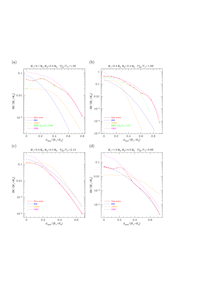
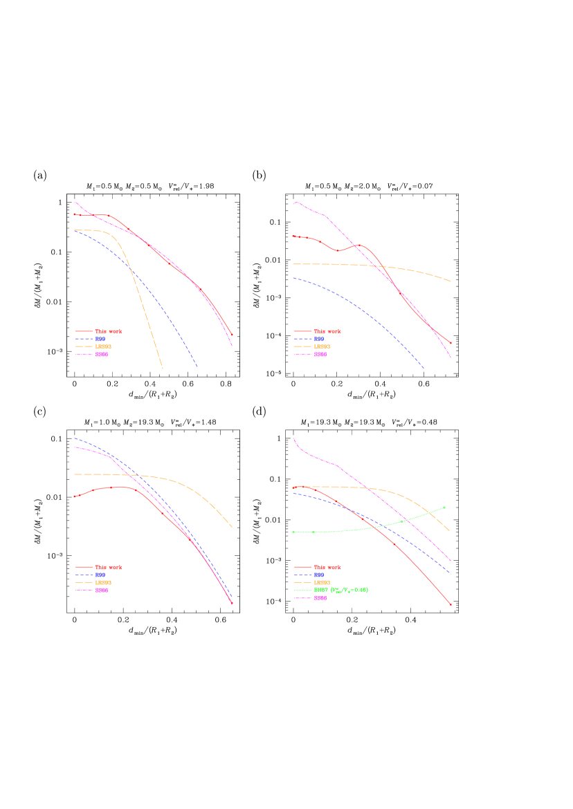
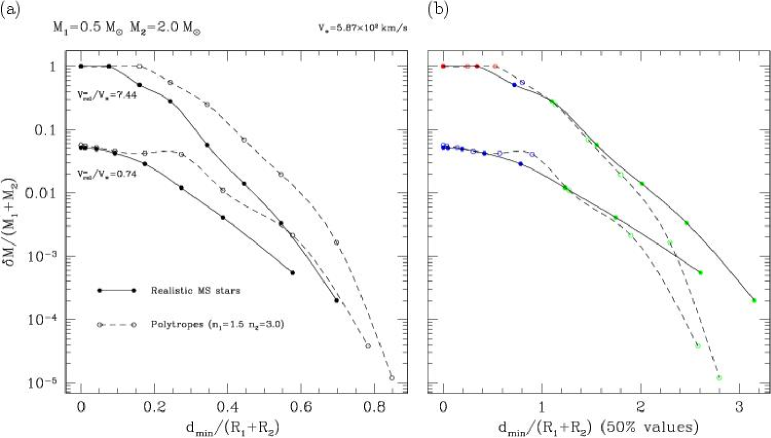
In Fig. 11, we show some selected cases for which we expect a good agreement with the literature results. There are however some exceptions that we explain in the caption of this figure. In Fig 12, more extreme comparisons are made. With Fig. 13, we concentrate on comparisons with simulation results of LRS93.

After inspection of these plots and many others not shown here, the following comments can be made:

1. When comparing some of our simulations to other individual computations with very similar initial parameters, a comforting, if not surprising, agreement emerges. This is particularly true of results from BH87 and BH92 . The situation with LRS93 (Fig. 13) is more complicated and we discuss it in detail below.

2. The initial stellar structure plays a central role in determining the results. But this strong dependency may probably be compensated to a large amount by some “clever” parameterisation of the initial conditions (see below).

3. Fitting formulae can not be used as extrapolation tools. This means not only that we cannot trust them when applied to larger or smaller velocity, masses or impact parameter values than the ones the have been forged for, but also that they will fail at predicting outcomes for other stellar models.

4. Predictions from LRS93 and R99 formulae are generally quite different, even when applied to the parameter domain in which they should both be relevant. This may be due to variations in the stellar structure (the $M$–$R$ relation) and/or amplified from small differences at the SPH level by the fitting procedures themselves. This is another indications that such formulae should be use with extreme caution.

5. An unexpected result from these confrontations is that the best match at $d_{\mathrm{min}}/(R_{1}+R_{2})>0.15$ and $V_{\mathrm{rel}}^{\infty}\geq 1$ is obtained with the SS66 method, which incorporates nearly no real physics! Furthermore, some of the crudest assumptions it relies on, which are certainly to be blamed for its breakdown at low impact parameter may probably be improved on. An exploration of the real potentialities of this simple approach would be an interesting follow-up of the present study, mainly because it reduces stellar collisions to very simple considerations about momentum and energy conservation and could thus be a useful guide toward a deeper insight into these processes. Once again, this unexpectedly good agreement strongly hints toward the central importance of the stellar structure in collision simulations. We should add that the SS66 approach also apparently breaks down for very high velocities $V_{\mathrm{rel}}^{\infty}>10$ where it yields too small a mass loss as compared to our simulations. It is interesting to note that the parameter domain for which SS66 gives very good results is well suited for collisions occurring in dense galactic nuclei. It may thus be that this recipe, when complemented with some prescription describing the domain of complete disruption, can be made into a useful ingredient for the study of such systems.

Let’s now focus on to comparison with results of LRS93, illustrated by Fig. 13. This work is of special importance as it constitutes the only survey of some breadth, also including high-velocity encounters, published so far. These authors used Eddington models with $n=3$ polytropic density profiles and assumed $R_{\ast}\propto M_{\ast}^{0.8}$. Eddington models have a constant $\beta=P_{\rm gas}/P_{\rm tot}$; they can be parametrised by $\alpha=7.89(1-\beta)^{1/2}\beta^{-2}$. LRS93 further assume $q=M_{<}/M_{>}=\alpha_{<}/\alpha_{>}\leq 1$ where subscripts $<$ and $>$ indicate the more and less massive star in the encounter, respectively. LRS93 have parametrised their results through a set of formulae that give the fractional mass loss as a function of $q$, $\alpha_{>}$, $v_{\infty}:=V_{\rm rel}^{\infty}(GM_{>}/R_{>})^{-1/2}$ and $d_{\rm min}/(R_{<}+R_{>})$. When comparing our results to this parametrisation, we set $\beta_{>}:=2E_{>}/W_{>}$ where $E_{>}$ is the total energy of the massive star (thermal plus gravitational) and $W_{>}$ the gravitational contribution. This relation is exact for Eddington models and is used here to define some “effective” $\beta$ parameter. $\beta$ is very close to 1 for $M_{\ast}<10\,{\rm M}_{\odot}$, leading to small $\alpha$ values. Hence, most LRS93 results (with $\alpha_{>}=10$, panels a and c of Fig. 13) are adapted to $M_{>}\gg 10\,{\rm M}_{\odot}$. This probably explains why LRS93 get considerably more mass loss than us; their stellar model have little binding energy compared to our realistic MS stars. Indeed, the best agreement is reached with the few $\alpha_{>}=1$ models, see Fig. 13b,d. Also, we stress again that $n=3$ polytropes do not represent in a satisfactory way the mass distribution of any (evolved) MS star except, maybe, around $M_{\ast}=0.9$ (see appendix).

Figure 14: Fractional mass loss as obtained in simulations with polytropes (dashed lines) and realistic stellar models (solid lines). For the simulations with polytropes, we used models of indices $n=1.5$ and 3 for the small and the large star, respectively. The same M-R relation was used for both sets of simulations. In panel (a), we normalised the Keplerian closest approach distance by the sum of the total stellar radii, We note that, except for head-on collisions which result in the same mass-loss, polytropes lead to a systematic over-estimate of $\delta M$. This is probably due of less concentrated density structure of the $n=3$ polytrope as compared to a “real” $2\,{{\rm M}_{\odot}}$ star. In panel (b), we use the half-mass radii as a normalisation. In this representation, the agreement is much better up to $\sim 2(R_{1}^{\mathrm{(h)}}+R_{2}^{\mathrm{(h)}})$. The small bump on the low velocity curve for polytropes at $\sim 0.9(R_{1}^{\mathrm{(h)}}+R_{2}^{\mathrm{(h)}})$ is probably the sign that this collision is a two-stage merger, i.e., that a short-lived binary is formed at first periastron passage that merge into a single object at second passage. The symbol type indicates the outcome of the collision: triangle for a complete disruption, open square for a binary, filled square for a fly-by and round dot when only one star remains (merger or disruption of the smaller star).

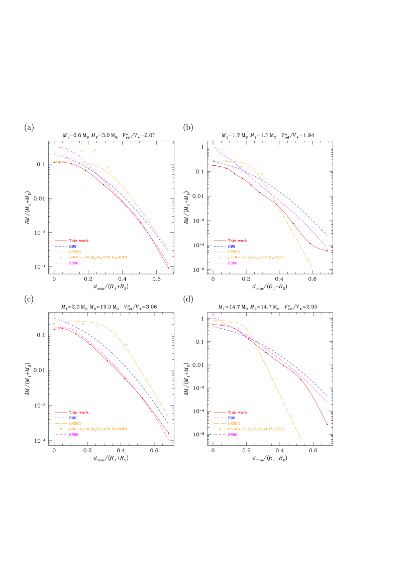
We now turn to an examination of the impact of the stellar models on collision results. In Fig. 14, we compare two sets of simulations. In both series, we computed collisions between stars of masses $0.5$ and $2.0\,{{\rm M}_{\odot}}$ for two different relative velocities and a sequence of impact parameters. In the first set, we used realistic stellar models, while in the second series, the small star is represented as a $n=1.5$ polytrope (which is a very good approximation) and the large one as a $n=3$ polytrope (a poorer model). Panel (a) in this diagram strongly confirms point 2 of the previous enumeration. Except for head-on encounters, the polytropic models systematically overestimate the mass-loss by factors as large as 5! This seems to strongly justify our use of realistic stellar structure instead of the traditional polytropes but panel (b) slightly weakens this statement. There we use the half-mass radii to normalise $d_{\mathrm{min}}$. This simple change of parameter, scales out the discrepancy to a large amount. Only for large $d_{\mathrm{min}}$ is the mismatch still strong (actually stronger!). This fact suggests that it could be possible to scale out much of the dependency on the stellar structure by use of some subtle parameterisation of the “closeness” of the collision that is a better representation than $d_{\mathrm{min}}/(R_{1}+R_{2})$ of the amount of stellar matter which is highly affected by the collision. In cases with stars of very different sizes, a good variable could be the mass fraction of the larger star inside $d_{\mathrm{min}}$ or some more realistic closest approach distance that includes corrections for non-Keplerian effects at small distances. In the same spirit, rather than using $V_{\mathrm{rel}}^{\infty}/V_{\ast}$ (or the half-mass version of this quantity), we could look for a parameterisation of the encounter’s severity that reflects the energy input compared to the total binding energy of the stars, for instance. In other words, our only hope to find a general description of our results that is both relatively simple and robust enough to allow some amount of extrapolation, is to trade apparent complexity in the results for physically motivated complexity in the parameters! At any rate clever parameterisations can possibly bring together the results of collisions for different stellar structures only as long as general quantities such as the mass and energy losses are concerned. Because the entropy and chemical profile of an evolved MS star is very different from a homogeneous polytrope, the structure and evolution of the collision products strongly depend on the use of realistic initial models, as demonstrated by Sills & Lombardi (1997).

Such remarks, as well as our comments on the strong limitations to the use of published fitting formulae (point 3, above) convinced us that any successful mathematical description of the collisions’ outcome should stem from physical considerations if it has to be used not only as a handy summary of the computed collisions but also to extrapolate to somewhat different initial conditions. Unfortunately, due to the complexity of the physical processes at play during collisions, such a “unifying” description seems very difficult to find and has escaped us so far. This pushed us to cover as completely as possible the relevant domain of initial conditions and motivated the use of an interpolation algorithm to determine the outcome of any given collision with parameters inside this domain.

3.3 Using the collision results in stellar dynamics simulations

3.3.1 The struggle for fitting formulae

Figure 15: Collisional fractional mass losses for four different $(M_{1},M_{2})$ pairs (values in ${{\rm M}_{\odot}}$). Simulation Data. White dots show the SPH simulations. The contours and colour maps are a bi-cubic interpolation of the SPH results. $\delta$ is the fractional mass loss $\delta=\delta M/(M_{1}+M2)$. Masses are in units of ${{\rm M}_{\odot}}$. In each frame, the upper left contour indicates fractional mass loss larger than 85 %.

Figure 16: Fractional mass loss ($\delta$) for all head-on, “zero-velocity” collisions. Here, $V_{\mathrm{cont}}$ is the contact velocity (at separation $R_{1}+R_{2}$). $\delta$ is not constant on lines of constant $M_{1}/M_{2}$.

Figure 17: Fractional mass loss for all collisions between a star of mass $19.3\,{{\rm M}_{\odot}}$ and stars that are at least 10 times less massive. Here we normalise the distance by $R_{2}$, the total radius of the large star. Points are colour-coded according to the kinetic energy of the impactor at contact (in solar units, $G{\rm M}_{\odot}^{2}/{\rm R}_{\odot}$).

Figure 18: Plots of the relative modification of the mass $M_{2}$ of the larger colliding star as a function of $d_{\mathrm{min}}$ and $V_{\mathrm{rel}}^{\infty}$. Mass decreases, colour-coded in red to yellow, are normalised as fractions of $M_{2}$. Mass increases, colour-coded in green tones are normalised as fractions of $M_{1}$. We choose this two different normalisations so these relative mass changes are always comprised between 0 and 1 in absolute value. $(M^{\prime}_{2}-M_{2})/M_{2}$ can me interpreted as the “fractional damage” caused by the “bullet” (small star) to the target, while $(M^{\prime}_{2}-M_{2})/M_{1}$ is the “efficiency” by which mass of the small star is added to the more massive one.

The result of a collision is described through a small set of quantities: the fractional mass loss $(M_{1}+M_{2}-{M_{1}}^{\prime}-{M_{2}}^{\prime})/(M_{1}+M_{2})$, the new mass ratio, the fractional loss of orbital energy and the angle of deviation of the relative velocity. Note that these values completely describe the kinematic outcome of a collision only if the centre-of-mass reference frame for the resulting star(s) (not including ejected gas) is the same as before the collision. Asymmetrical mass ejection violates this simplifying assumption by giving the resulting star(s) a global kick (Benz & Hills, 1987). However, we checked that the kick velocity is generally much lower than the relative velocity. Thus, this simplification, which greatly reduces the complexity of the situation, should not lead to an important bias in the global influence of collisions in the energy balance of a star cluster.

We have kept the final SPH particle configuration for (nearly) all our simulations. This would allow us to re-analyse these files and extract other quantities of interest, like the amount of rotation imparted by the collision, a quantity worth investigating because it can deeply influence the subsequent evolution of the star(s) (Maeder & Meynet, 2000; Sills et al., 2001) and lead to observational signatures that would reveal the importance of collisions and close encounters in given environments (Alexander & Kumar, 2001). Another interesting issue is the resulting internal stellar structure. This is key to a prediction of the subsequent evolution and observational detectability of collision products (Sills et al., 1997, 2001, for instance). Unfortunately, according to Lombardi et al. (1999), low resolution and use of particles of unequal masses can lead to important spurious particle diffusion in SPH simulations so that our models are probably not well suited for a study of the amount of collisional mixing, for instance.

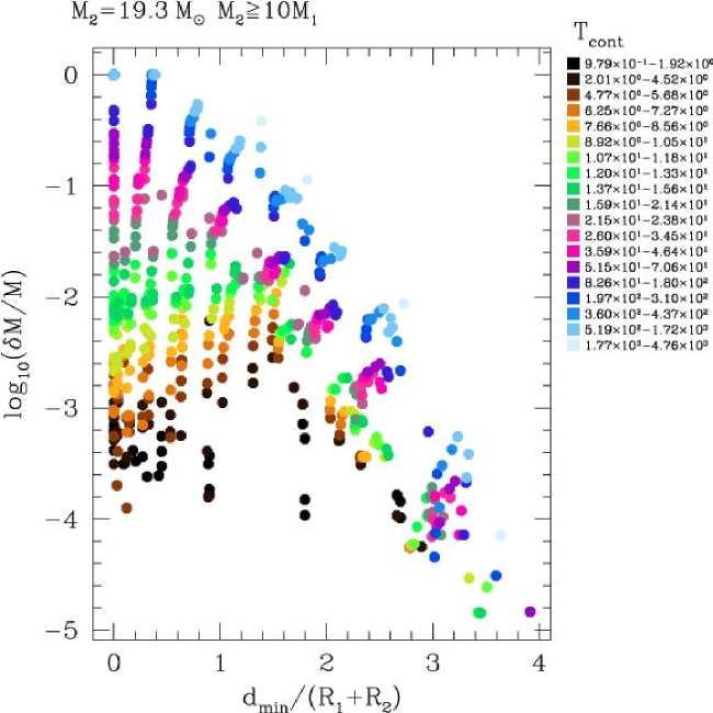
Fig. 15 shows the (interpolated) fractional mass loss in the $(d_{\mathrm{min}},\,V_{\mathrm{rel}}^{\infty})$ plane for various $(M_{1},M_{2})$ pairs. Note how the “landscape” changes from one choice of $(M_{1},M_{2})$ to another one. Such relatively complex structure obviously is a challenge to attempts of describing the results by fitting formulae.

Let’s report some unsuccessful attempts at finding easy-to-express regularities in the simulation data. We first convinced ourselves that the outcome of a collision does depend on both stellar masses and not only on the mass ratio $q=M_{1}/M_{2}$. This is demonstrated in Fig 16 in which we plot the total fractional mass loss for head-on mergers with $V_{\mathrm{rel}}^{\infty}\simeq 0$. If this quantity depended on $M_{1}$ and $M_{2}$ only through $q$, we would obtain constant $\delta$ values along diagonals, which is not the case. Fig. 17 depicts another wrong guess, namely that for stars of very different sizes, the mass loss would only depends on the kinetic energy of the impactor (and on $d_{\mathrm{min}}$) and not on its mass. There is not much interest in explaining in detail all the strategies we have tried to reduce our huge dataset to a more manageable mathematical formulation. As a last illustration of the difficulty of such a programme, let’s mention our attempt at a global parameterisation of the mass-loss curves. We found a 3-parameter formula that allowed good fits of individual $d_{min}/(R_{1}+R_{2})\longrightarrow\delta M/(M_{1}+M_{2})$ relations (for fixed $M_{1}$, $M_{2}$ and $V_{\mathrm{rel}}^{\infty}$). This looked very promising but we were left with 1180 sets of parameters to be adjusted in turn by some “meta-formula”, with the added difficulty that they displayed a lesser level of regularity than the raw collisional data itself. This proved unmanageable. Furthermore, this parameterisation had no sound physical justification.

To end this subsection on a more positive note, let’s turn to Fig. 18. In this diagram, we plot the relative mass gain or loss for the larger star, $\delta_{2}$, as a function of the usual half-mass normalised $\lambda$ and $\nu$. The figures are remarkably smooth in the sense that collisions with comparable mass ratios, but otherwise different $M_{1}$ and $M_{2}$, and same $(\lambda,\nu)$, produce very similar $\delta_{2}$. There is thus some hope that, in further investigations, we could discover some “universal” $\delta_{2}=\delta_{2}(q,\nu,\lambda)$ relation to describe this regularity. Such a description would be particularly useful to explore, with analytical or semi-analytical models, the possibility of run-away merging sequences in the evolutions of dense clusters. Using realistic SPH results to re-examine these scenarios is one important application of the present work (see Sec. 1.1).

3.3.2 Interpolation of the collision results

Figure 19: Delaunay triangulation in two dimensions. In our interpolation method we would get the value for the point $P$ (small square) from data points 1, 2 and 3 that are the vertices of the triangle $P$ lays in. Although they are much closer to $P$ than 1 or 3, points 4 and 5 would not contribute at all!

Figure 20: Four slices through our interpolation grid for the collisional fractional mass loss. We performed cuts that correspond to $(M_{1},M_{2})$ values close to those of Fig. 15. $\delta$ is the fractional mass loss $\delta=\delta M/(M_{1}+M2)$. Masses are in units of ${{\rm M}_{\odot}}$. The Delaunay interpolation produces some artifacts at low and high relative velocities, in particular for the top-left and bottom-right panels (compare with Fig. 15). This is due to the simplices being very elongated near the border of the convex hull of our data (in four dimensional space).

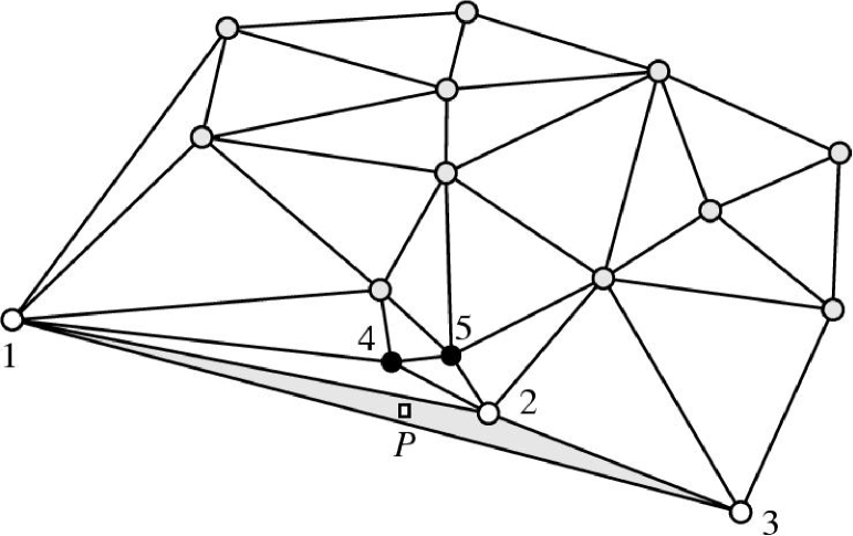
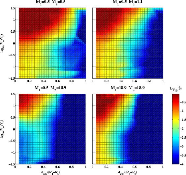
Being unable to distillate the results of our SPH simulations into any compact mathematical formulation without losing most of the information, we resorted to the following interpolation strategy. In the 4D initial parameter space, the simulations form a irregular grid of points. We compute a Delaunay triangulation of this set (Sedgewick, 1988, Chap. 28) using the program QHULL (Barber et al., 1996) which allows us to interpolate the results onto a regular 4D grid. To evaluate the value of any of the four quantities that summarise the outcome of a collision, $\mathfrak{Q}$, we first find the simplex $\mathcal{S}$ of the triangulation, if any, that contains the 4D point $P$ of the initial conditions of the collision. This simplex has 5 vertices: $Q_{i},i=1\ldots 5$. By removing one of these vertices, say $Q_{k}$ and replacing it by $P$, one forms another, smaller simplex $\mathcal{S}_{k}$ that is contained in $\mathcal{S}$. We compute the interpolated value of $\mathfrak{Q}$ at point $P$, $\tilde{\mathfrak{Q}}(P)$ from its values at the vertices $Q_{i}$, $\mathfrak{Q}(Q_{i})$ by linear combination with weights $V_{\mathcal{S}_{k}}/V_{\mathcal{S}}$ where $V_{\mathcal{S}}$ stands for the (hyper-)volume of $\mathcal{S}$. Of course, this procedure does not allow extrapolation outside the convex hull of our simulation initial conditions. Another, more tricky problem is that, near the borders of this convex hull, simplices can be very elongated which means that the interpolations can be done with data points corresponding to very remote initial conditions instead of using more local information. This is illustrated, for two dimensions, in Fig. 19.

However, we did not find a better procedure. We tried to use a kernel-based method, à la SPH, but it produced very poor results. The main problem with this class of algorithms is to adapt locally the 4 independent axis of the kernel ellipsoid in such a way that only neighbouring data points contribute to the evaluation at a given point. Defining “neighbours” is unfortunately not obvious in a parameter space with no natural metrics.

The quality of the data obtained through our interpolation mechanism is illustrated on Fig. 20. It shows four 2D slices of the fractional mass loss interpolated onto the 4D grid. Each slice corresponds to a $(M_{1},\,M_{2})$ pair chosen as to be as close as possible to the values used for Fig. 15, allowing a direct comparison. The general dependency of the mass loss on impact parameter and relative velocity is well reproduced but some details are smoothed out while small artifacts have appeared near the borders of the domains for the reason explained above. We interpret the horizontal “peninsula” of high mass loss for $M_{1}=M_{2}=0.5\,{\rm M}_{\odot}$ as the result of the interpolation between a simulation which was integrated long enough for complete merger (visible on Fig. 15 for the lowest relative velocity value at $d_{\rm min}/(R_{1}+R_{2})=0.8$) and led to relatively high mass loss and others which were stopped at an earlier phase (unmerged binary).

The table thus computed is the backbone of the routine that implements stellar collisions in our Monte Carlo simulations of stellar clusters. Collision outcome quantities are indeed easily obtained through a second, much quicker, interpolation stage using this regular grid. Of course, extrapolation prescriptions have to be specified for events whose initial conditions fall outside the convex hull of the SPH simulation points. Most commonly, this happens when a collisionally produced star with mass outside the $0.1$–$74\,{{\rm M}_{\odot}}$ range experience a further collision. In such cases, we try to re-scale both masses while preserving $M_{1}/M_{2}$ to get a “surrogate collision” lying in the domain covered by the SPH simulations. If $V_{\mathrm{rel}}$ is too low or too high, we increase or decrease it to enter the simulation domain. In its present state, this treatment of “extreme” velocities is not completely satisfying. At very high $V_{\mathrm{rel}}$, our data do not show convergence toward a unique mass loss curve. Instead, the domain of complete disruption keeps extending to higher and higher impact parameters with a progressive steepening of the mass loss curves for “fly-bys”. At very small velocities, the values of the table can be trusted only when no binary has formed or if the binary evolution has been followed up to merging. In case of binary formation, some constant fractional mass loss could be used in order to reflect our finding that the process of binary merging, that requires more and more pericentre passages for larger and larger $d_{\mathrm{min}}$, eventually leads to an amount of mass loss relatively independent of this impact parameter. A more precise determination of the maximal $d_{\mathrm{min}}$ that still leads to binary formation for small initial velocities would allow us to know where to switch between this prescription and interpolation in the table. Finally, cases with too high $d_{\mathrm{min}}$ are treated as purely Keplerian hyperbolic encounters with no mass loss, which is a very good approximation. Recently, in the frame of our work on collisional run-away formation of very massive stars, we have implemented a few more small tricks to complement our “blind” interpolation routine and reduce its artifacts (Freitag et al., 2005b, a).

An important aspect of the work reported here is that we make the data describing the initial conditions and outcome of all our simulations available on the web, on the site of the “MODEST” working group on stellar collisions at http://obswww.unige.ch/~freitag/MODEST_WG4/FB_Collision_Data/. We provide a description of the outcome of a given collision in terms of the number and masses of star(s) at the end of the simulation and their orbital properties. Colleagues are invited to develop their own methods to use this data and share their experience with others, including the authors of the present paper. Files containing detailed information for all SPH particles at the end of a simulation are available upon request to MF.

4 Conclusions and future work

In this article, we presented a large set of simulations of collisions between two main sequence stars. More than 14 000 SPH simulations have been computed over about four years to complete that database. Initial conditions span $M_{\ast}=0.1-75\,{\rm M}_{\odot}$ for the stellar masses, impact parameters corresponding approximately to $d_{\mathrm{min}}/(R_{1}+R_{2})=0-0.9$ and relative velocities at infinity ranging, more or less, from 0.03 to 30 times the stellar escape velocity. This represents a effort of unprecedented breadth in this field.

Our motivation in this work was to incorporate the effects of stellar collisions into models of dense stellar systems like galactic nuclei with as much realism as possible. To reach this goal we developed a module that interpolates between our results to predict the outcome of any collision with initial conditions inside the (large) domain of parameter space we explored. Results of our dynamical simulations of dense clusters including collisions are presented elsewhere (Freitag & Benz 2001a, 2002; Rasio et al. 2004; Freitag et al. 2004b, a, 2005b, 2005a).

The quest for a handy mathematical description of these results has been unsuccessful so far. This was a source of disappointment but we hope that further study of our simulation data will eventually reveal some way of casting our results in a compact and physically enlightening formulation. Exploring when and why the excellent match with the SS66 prescription is found is a possible way to this goal.

Beyond the scientific exploitation of this important database, –either to develop a better understanding of the physics of collisions or as an ingredient for collisional stellar dynamics studies– we are aware that other kinds of stellar collisions, not treated here, are also of great astrophysical interest. First, in galactic nuclei, collisions with red giants are certainly more frequent than MS-MS encounters. So we should assess the importance of this process (for stellar evolution and stellar dynamics) and, if needed, compute a set of simulations similar to the one presented here. This would complement the work of Bailey & Davies (1999). Collisions with compact remnants should also be taken into account as they may be of great importance in producing peculiar objects.

Our work is not well adapted to the physical conditions that are typical in globular clusters. Indeed, we did not study with particular care the low velocity, quasi parabolic encounters, by far the most common in those environments. However, they have already been quite thoroughly studied by other researchers. The conditions for tidal binary formation are probably better determined using other methods and their long term evolution, whose nature and result is still debated (Mardling, 1995a, b), extends over much too many hydrodynamical time scales to be tackled by SPH. Still in the domain of globular clusters, the study of hydrodynamical effects (including direct collisions) in interactions with or between binary stars is still in its infancy (Goodman & Hernquist, 1991; Davies et al., 1993, 1994).

Finally, going back to galactic nuclei in which we are mostly interested, let’s mention that the connected problem of the destructive close encounter between a central massive black hole and a star, even though it has been the focus of many papers (Carter & Luminet, 1983; Bicknell & Gingold, 1983; Evans & Kochanek, 1989; Laguna et al., 1993; Fulbright, 1996; Marck et al., 1996; Ayal et al., 2000; Bogdanović et al., 2004, and many others), has still not been explored systematically. For instance, all studies so far have assumed simplified stellar models. In this problem, however the main uncertainties probably lurk in the post-disruption evolution of the stellar gas, rather than in the “collision” process itself.

Appendix A Smoothed Particle Hydrodynamics stellar models.

A.1 Stellar structure used in the simulations

Figure 21: Density profiles for realistic star models (Schaller et al., 1992; Charbonnel et al., 1999) for low (top) and high (bottom) mass stars. The dashed lines are polytropic models for $n=1.5$, 3 and 4, in order of increasing concentration. Below $0.4\,M_{\odot}$, the density structure is well represented by a polytrope with $n=1.5$ but no good polytropic fit is possible for higher masses.

Figure 22: SPH realisation of a $3\,M_{\odot}$ stellar model with $\sim$2000 particles. Round dots show the positions of SPH particles with a symbol surface proportional to the particle’s mass. The big dashed circle shows the size of the star according to the structure model. Plain line circles depict the concentric spheres on the surface of which the particles’ centres are placed. Particles on the $x,y>0$ corner of the diagram have been removed to show the actual half-size of particles on each sphere (dotted circles of radius $h$).

Figure 23: Comparison between the theoretical internal structure of a $2\,M_{\odot}$ stellar model (solid lines) and SPH realisations of it with increasing number of particles (dashed and dotted lines). We show the mass density (left column) and the internal energy (right column). In the top row, we use the radius as the abscissa, while we use the enclosed mass for the diagrams of the bottom row. The top plots show that the outermost part of the star are poorly represented. However, it is clear from the bottom plots that only a tiny mass fraction suffers from this mismatch. The SPH profiles are the kernel-interpolated values along the line $z=0$.

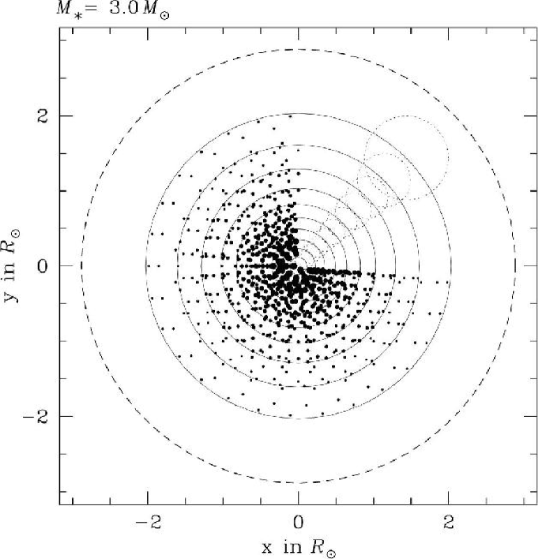
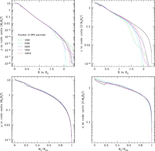
In Fig. 21, we show the density profiles for some realistic models for MS stars and compare them with polytropic stars. It is readily seen that for $M>0.4\,M_{\odot}$, stellar structures are highly non-homologous and that polytropes do not match, even if allowance is made for a $M$-variable $n$ index. If such a fit is required anyway, a value of $n\simeq 3.5$ seems more appropriate for $M\geq 1\,M_{\odot}$ than the commonly used $n=3$.

An SPH particle configuration for a star is illustrated on Fig. 22. One sees that the outermost layers of the star are very poorly modelled, with a clear failure at precisely reproducing the real stellar radius. Fig. 23 is a comparison between the density and internal energy profiles of two stellar models and their SPH approximation for increasing number of particles.

A.2 Choice of the particle number

Figure 24: Study of the dependency of collision results on the particle number for 4 sets of collision simulations. (a) Fractional mass loss. (b) Fractional loss in orbital energy. The simulation set with $M_{2}=19.3\,M_{\odot}$ is not reported here because it results in a merger ($\delta E_{\mathrm{orb}}/E_{\mathrm{orb}}=1$). (c) Deviation of the collisional deflection angle $\theta_{\rm coll}$ from the value for pure Keplerian point-mass trajectory $\theta_{\rm grav}$.

In Fig. 24, we show how the overall results of SPH collision simulations (mass and energy loss, deflection angle) depend on the resolution, i.e. the number of particles used to represent the stars. We considered resolution ranging from 1000$+$2000 to 2000$+$32 000 particles.

Appendix B Results of SPH simulations

B.1 A few specific collision simulations

Figure 25: Collision between two $2.0\,M_{\odot}$ stars at $V_{\mathrm{rel}}^{\infty}/V_{\ast}=0.77$ ($465$ km s^-1) and $d_{\mathrm{min}}/(R_{1}+R_{2})=0.1$. Each plot show the position, projected onto the orbital plane, of SPH particles that lie close to this plane. Beware that the length scale may change from frame to frame. This collision creates a merged star with mass $3.81\,M_{\odot}$. The particles are colour-coded according to their rank in the initial stellar models.

Figure 26: Collision between stars of masses 1.0 and $3.0\,M_{\odot}$ at $V_{\mathrm{rel}}^{\infty}/V_{\ast}=0.07$ ($44$ km s^-1) and $d_{\mathrm{min}}/(R_{1}+R_{2})=0.0$. This collision creates a merged star with mass $3.80\,M_{\odot}$. The particles are colour-coded according to their rank in the initial stellar models.

Figure 27: Collision between stars of masses $0.4\,M_{\odot}$ and $4.0\,M_{\odot}$ at $V_{\mathrm{rel}}^{\infty}/V_{\ast}=3.24$ ($2180$ km s^-1) and $d_{\mathrm{min}}/(R_{1}+R_{2})=0.04$. The colours code the gas density. This collision results in a merged star with mass $3.75\,M_{\odot}$.

Figure 28: Snapshot of the collision simulation of Fig. 27 at later stage. One sees the small star spiralling into the centre of the larger star. Panel (a): density plot. Panel (b): Velocity plot with colours indicating the radial position of each particle in the initial stellar models. Particles from the large star are coded in red to yellow, from centre to surface. Particles from the small star are coded in dark to light green. The small dots are the position of the particles. The velocity scale is given by the horizontal line segment at the bottom right of the diagram.

Figure 29: Collision between stars of masses $1.7\,M_{\odot}$ and $7.0\,M_{\odot}$ at $V_{\mathrm{rel}}^{\infty}/V_{\ast}=3.68$ (2620 km s^-1) and $d_{\mathrm{min}}/(R_{1}+R_{2})=0.0$. Not only is the small star still bound as it emerges from the collision, but it has also accreted some gas from the larger star so that its final mass is $1.74\,M_{\odot}$! Much damage has been caused to the larger star, though, which has lost all but $1.94\,M_{\odot}$.

Figure 30: Same collision as in Fig. 29. In this series of plots, Positions and densities are relative to the particle that lies at the centre of the larger star at the end of the simulations. A constant length scale is applied to all diagrams but the last one which shows a larger view. The velocity scale is adapted from frame to frame.

Figure 31: Collision between stars of masses $0.5\,M_{\odot}$ and $2.0\,M_{\odot}$ at $V_{\mathrm{rel}}^{\infty}/V_{\ast}=4.48$ (2620 km s^-1) and $d_{\mathrm{min}}/(R_{1}+R_{2})=0.15$.

Figure 32: Enlargements of the last frame of Fig. 31. Position and velocities are relative to the particle with the highest density in each panel. Panel (a): remaining of the large star ($1.53\,M_{\odot}$). Panel (b): remaining of the small star ($0.05\,M_{\odot}$).

Figure 33: Collision between stars of masses $0.4\,M_{\odot}$ and $1.7\,M_{\odot}$ at $V_{\mathrm{rel}}^{\infty}/V_{\ast}=3.80$ (2180 km s^-1) and $d_{\mathrm{min}}/(R_{1}+R_{2})=0.11$.

Figure 34: Continuation of the sequence of Fig. 33.

Figure 35: Enlargements of the last frame of Fig. 34. Position and velocities are relative to the particle with the highest density in each panel. Panel (a): surviving core of the large star, a $1.26\,M_{\odot}$ rotating star. Panel (b): remaining of the core of the small star, an unbound expanding gas cloud. The velocity of this cloud in the centre-of-mass reference frame of the collision is nearly 1000 km s^-1 while the velocity of the small star was initially 1770 km s^-1.

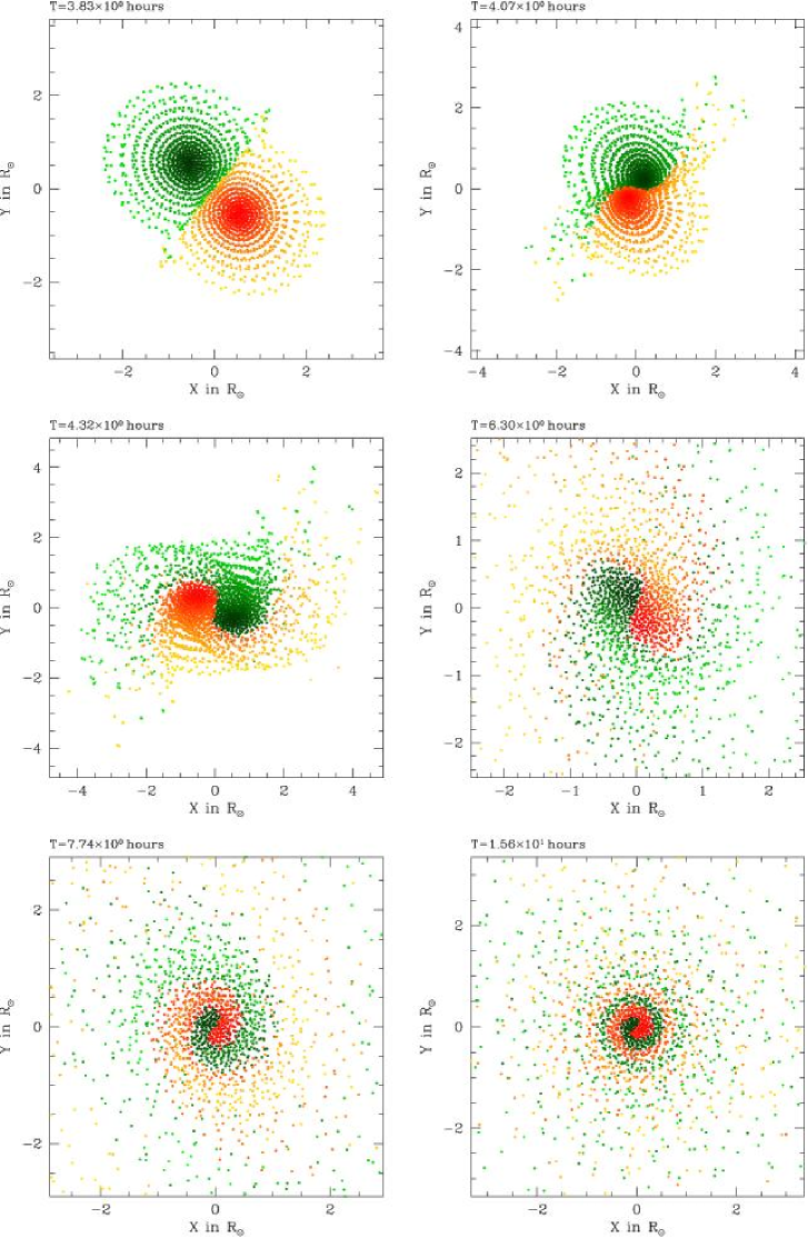
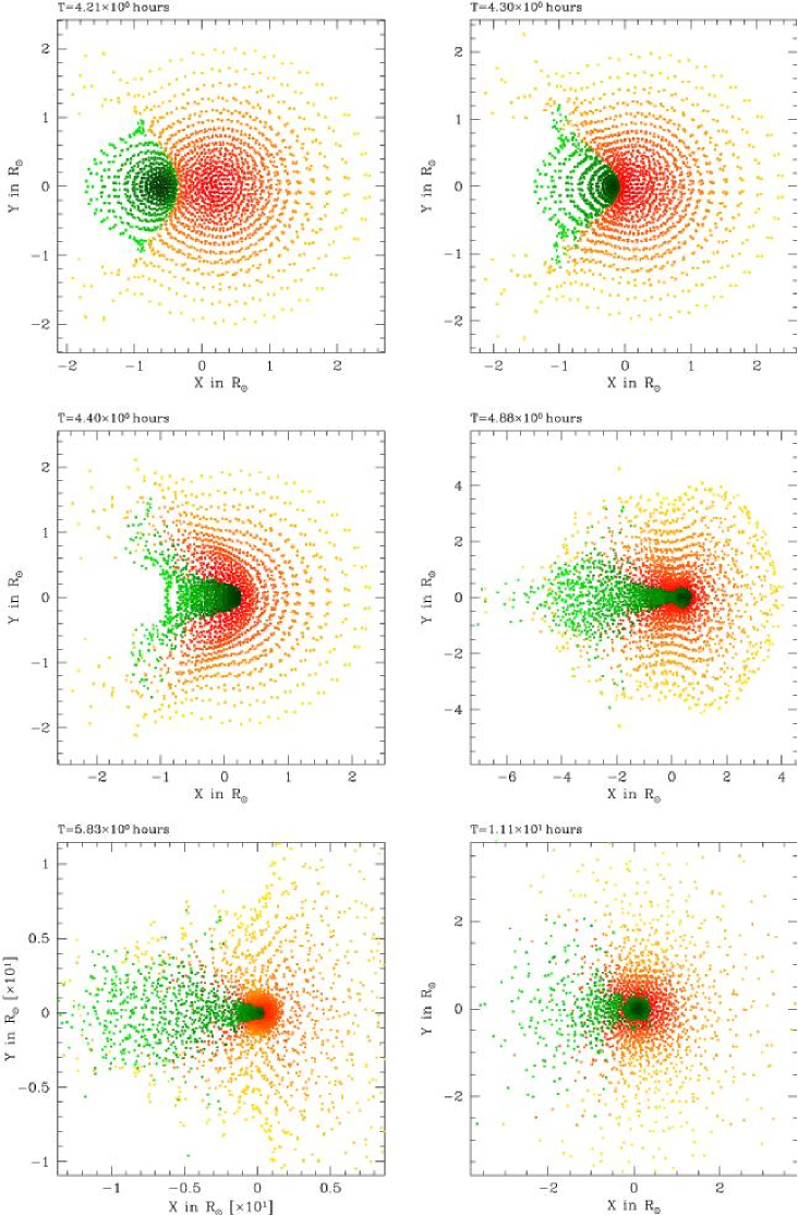
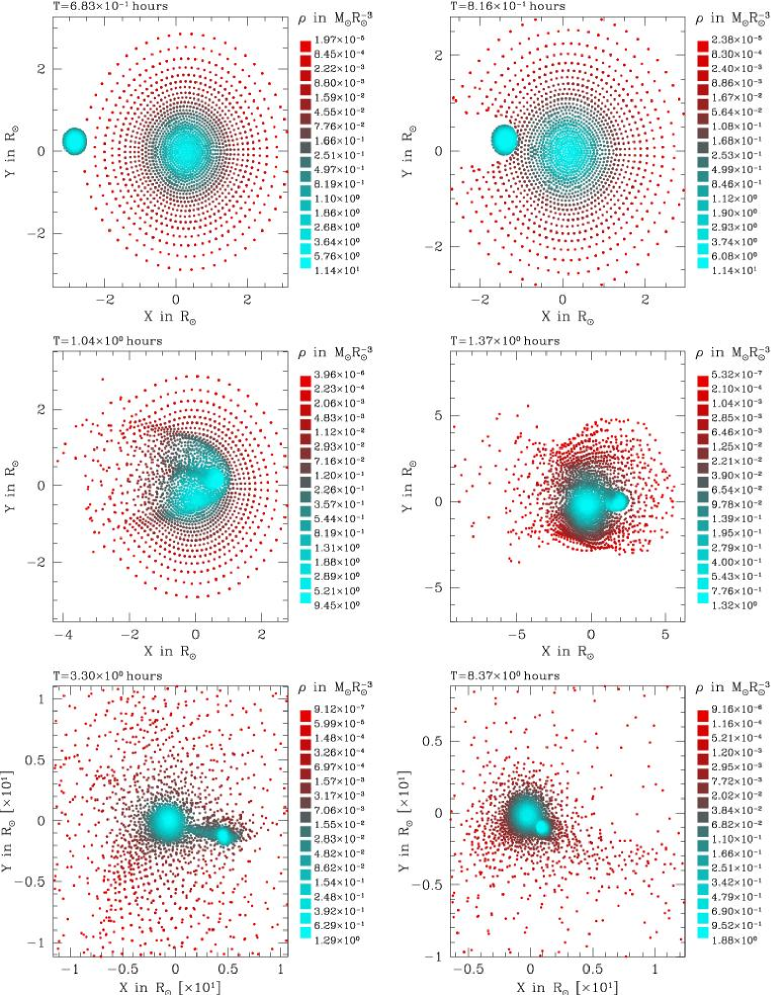
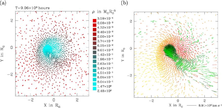
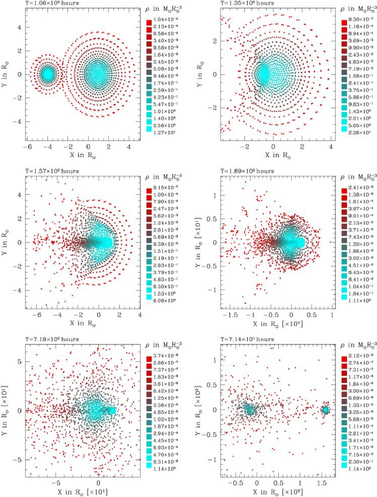
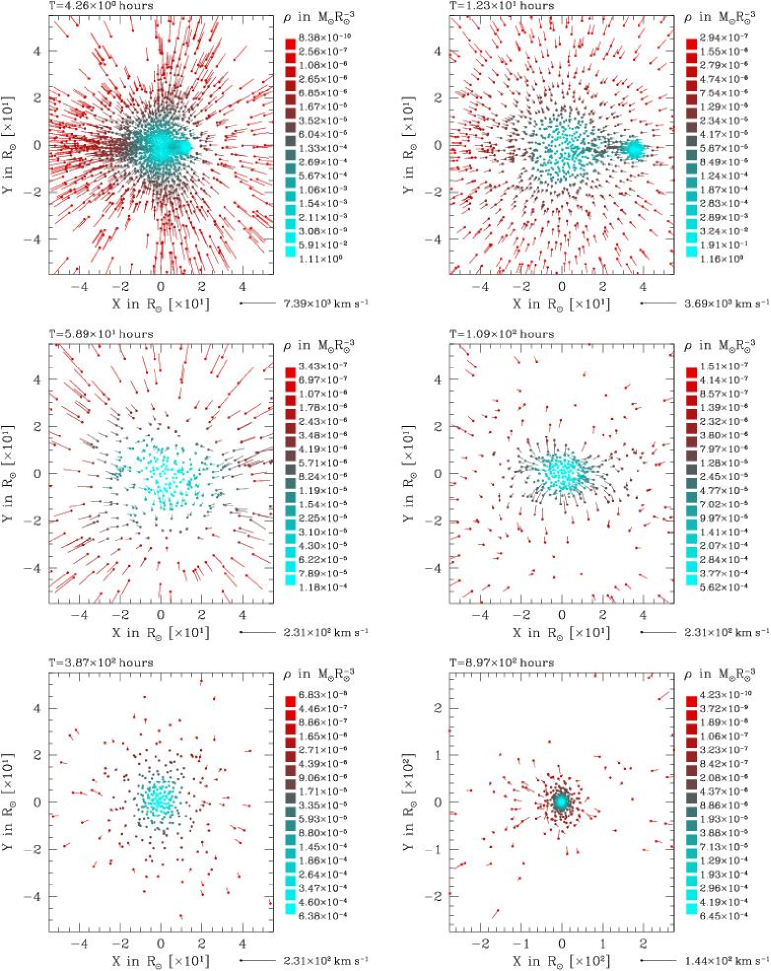
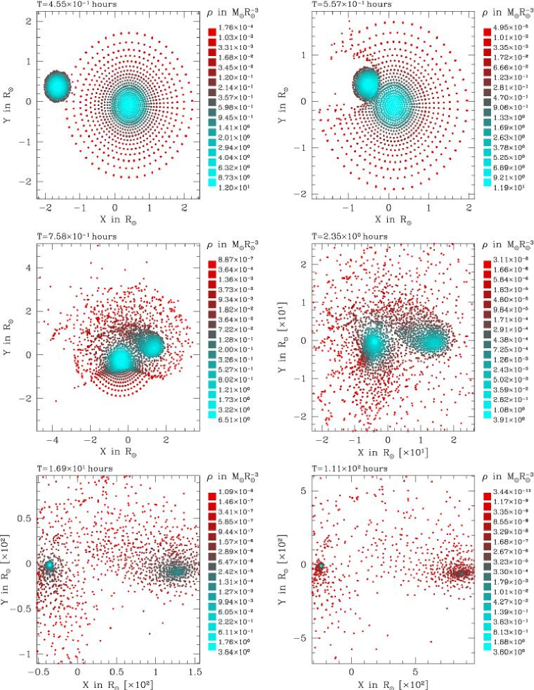
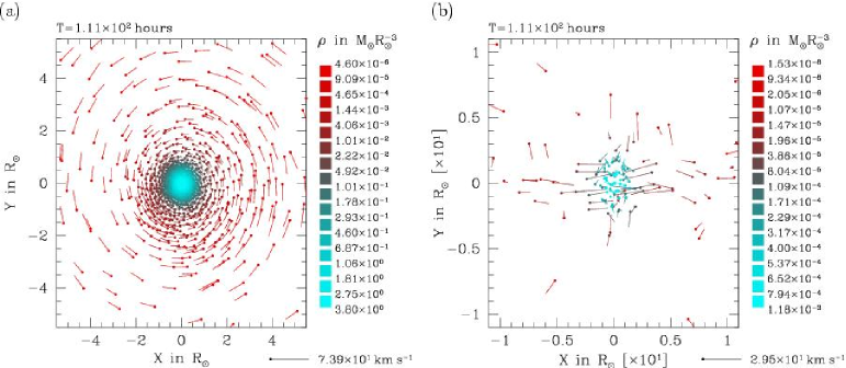
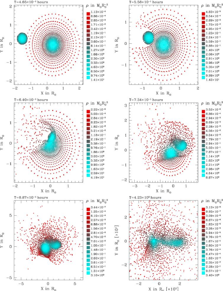
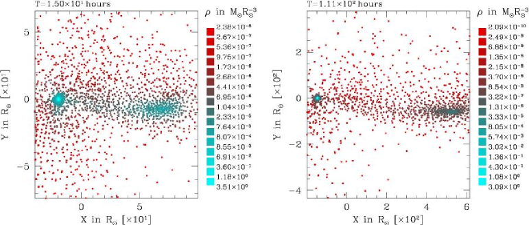
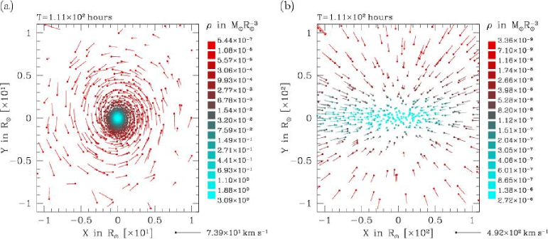
Precise descriptions of the physical mechanisms at play during stellar collisions have already been published (Benz & Hills, 1987, 1992; Lai et al., 1993; Lombardi et al., 1996). In this subsection, we just highlight a few particular collisions from our survey for illustration purposes. We do not particularly concentrate on “classical” typical cases because they have been well covered in these previous works. Instead, we concentrate on simulations with parameters lying on the border-lines of the various regimes. Many of them have been re-computed in order to test surprising results. Indeed, for lack of sufficient disk space for data storage, only the final “state” of each SPH simulation was conserved for most runs. So, when any doubtful result appeared, we had to re-compute the complete simulation and write the data to disk frequently in order to understand the evolution of the system.

In Fig. 25, we show an off-axis low velocity encounter between identical stars. As the impact parameter is small, the stars merge together after the first periastron passage. The colour mapping used in these diagrams allow to trace each particle back to its initial radial position in the colliding stars. Despite the rather low resolution (about 8000 particles in total) a tighter and tighter spiral pattern is clearly visible. As explained by Lombardi and collaborators, in low velocity collisions, specific entropy $s$ is nearly conserved as shock heating is weak, and, as stability of the resulting star imposes $\mathrm{d}s/\mathrm{d}r>0$, low entropy material that was initially at the centre of the stars, settles in the centre of the merged object. In fact, for such gentle encounters, one can even predicts the final material stratification by sorting mass elements from the two stars in order of increasing entropy (Lombardi et al., 1996, 2002, 2003). A consequence of this mechanism is that, in mergers between stars with unequal masses, the core of the smaller one, having the lowest entropy, sinks to the centre of the merger. This is also what happens in the two collisions depicted in Figures 26, 27 and 28. The second collision is an example of a high velocity merger which produce an object with a total mass slightly lower than those of the initial larger star. Such a case lies in the tip of merger region in a diagram like those in Fig. 9 of the main paper.

In Figures 29 and 30, we display snapshots from one of the few head-on collisions in which the small star pass through the large one and remains essentially intact. A further peculiarity of this collision is its relatively large mass ratio: $q=0.24$. No collision with a larger $q$ resulted in a similar outcome. Figures 31 and 32 depict a more typical “fly-by” in the sense that it has non-vanishing impact parameter. However, this high velocity encounter lies very close to the strip of complete disruption of the small star. For this particular simulation, the small star loses more than 89 % of its mass! The remaining cloud has a very low central density, around $10^{-4}$ g cm^-3. It is made of only 187 particles so simulations with higher resolution are clearly needed to confirm that the production of such tiny survivors is not a numerical artifact. It is however unlikely that such small, rarely formed objects, may have important astrophysical relevance, either as detectable “exotic” stars or dynamically.

We finally present a collision from the high velocity, 1-star branch, i.e. a case of collisionally induced evaporation of the small star. We particularly checked that this kind of outcome was real and not some artifact cause by our analysis software. Indeed, during these verifications, we noted that many cases of nearly complete destruction of the small star like the one described in Figures 29 and 30 were mis-interpreted because our code missed the second, much lower, density peak. Consequently, we had to re-analyse all high $\nu$ collisions that were reported to result in the disruption of the small star. We conclude that although the precise location of its right (large $d_{\mathrm{min}}$) edge may depend on numerical issues (resolution, analysis procedure), the 1-star branch is real. Inspecting the last frames of Figures 33 and 34 and Fig. 35 makes this fact obvious. Furthermore, such collision results have been reported by Lai et al. (1993).

B.2 Examples of mass and energy loss results

Figure 36: Relative mass and kinetic energy losses for all collision simulations between stars of masses $0.5$ and $12\,{\rm M}_{\odot}$ (column (a)) and $12$ and $12\,{\rm M}_{\odot}$ (column (b)). Half-mass radii are used to normalise parameters. $T_{\mathrm{cont}}$ is the orbital kinetic energy at “half-mass contact” (separation equal to $R_{1}^{\mathrm{(h)}}+R_{2}^{\mathrm{(h)}}$), assuming purely Keplerian acceleration. For very small $V_{\mathrm{rel}}^{\infty}$, all encounters result either in mergers or in bound binaries that should eventually merge together, with $\delta T_{\mathrm{cont}}/T_{\mathrm{cont}}=1$ and a higher $\delta M/(M_{1}+M_{2})$ as consequences. At high velocities, the domain of 100 % complete energy loss extends to $d_{\mathrm{min}}$ values where mass loss is only partial. This is due to the complete disruption of the smaller star after it emerges from the large one. The shoulders on the low velocity mass loss curves are due to the formation and subsequent merging of a binary.

Fig. 36 shows the energy and mass loss curves for the simulations of collisions between stars with $(M_{1},\,M_{2})=(0.5,\,12)\,{\rm M}_{\odot}$, and $(12,\,12)\,{\rm M}_{\odot}$. Similar curves for other $(M_{1},\,M_{2})$ couples are available upon request to MF. The can also easily be drawn using the complete tables of collision results available on-line.

References

- Alexander (1999) Alexander T., 1999, ApJ, 527, 835
- Alexander & Kumar (2001) Alexander T., Kumar P., 2001, ApJ, 549, 948
- Arabadjis (1997) Arabadjis J. S., 1997, PhD thesis, University of Michigan
- Ayal et al. (2000) Ayal S., Livio M., Piran T., 2000, ApJ, 545, 772
- Bahcall & Wolf (1976) Bahcall J. N., Wolf R. A., 1976, ApJ, 209, 214
- Bahcall & Wolf (1977) —, 1977, ApJ, 216, 883
- Bailey & Davies (1999) Bailey V. C., Davies M. B., 1999, MNRAS, 308, 257
- Barber et al. (1996) Barber C. B., Dobkin D. P., Huhdanpaa H. T., 1996, ACM Transactions on Mathematical Software, 22, 469
- Barth (2004) Barth A. J., 2004, in Coevolution of Black Holes and Galaxies, from the Carnegie Observatories Centennial Symposia., Ho L., ed., Cambridge University Press, p. 21
- Barth et al. (2004) Barth A. J., Ho L. C., Rutledge R. E., Sargent W. L. W., 2004, ApJ, 607, 90
- Begelman & Rees (1978) Begelman M. C., Rees M. J., 1978, MNRAS, 185, 847
- Benz (1990) Benz W., 1990, in Numerical Modelling of Nonlinear Stellar Pulsations Problems and Prospects, Buchler J. R., ed., pp. 269–288
- Benz et al. (1990) Benz W., Cameron A. G. W., Press W. H., Bowers R. L., 1990, ApJ, 348, 647
- Benz & Hills (1987) Benz W., Hills J. G., 1987, ApJ, 323, 614
- Benz & Hills (1992) —, 1992, ApJ, 389, 546
- Benz et al. (1989) Benz W., Hills J. G., Thielemann, 1989, ApJ, 342, 986
- Bicknell & Gingold (1983) Bicknell G. V., Gingold R. A., 1983, ApJ, 273, 749
- Binney & Tremaine (1987) Binney J., Tremaine S., 1987, Galactic Dynamics. Princeton University Press
- Bogdanović et al. (2004) Bogdanović T., Eracleous M., Mahadevan S., Sigurdsson S., Laguna P., 2004, ApJ, 610, 707
- Bressan et al. (1993) Bressan A., Fagotto F., Bertelli G., Chiosi C., 1993, A&AS, 100, 647
- Carter & Luminet (1983) Carter B., Luminet J.-P., 1983, A&A, 121, 97
- Chabrier & Baraffe (1997) Chabrier G., Baraffe I., 1997, A&A, 327, 1039
- Chabrier & Baraffe (2000) —, 2000, ARA&A, 38, 337
- Charbonnel et al. (1999) Charbonnel C., Däppen W., Schaerer D., Bernasconi P. A., Maeder A., Meynet G., Mowlavi N., 1999, A&AS, 135, 405
- Colgate (1967) Colgate S. A., 1967, ApJ, 150, 163
- Combes (2001) Combes F., 2001, in Advanced Lectures on the Starburst-AGN Connection, INAOE, June 2000, Aretxaga I., Mújica R., Kunth D., eds., World Scientific, p. 223
- Courvoisier et al. (1996) Courvoisier T. J.-L., Paltani S., Walter R., 1996, A&A, 308, L17
- David et al. (1987a) David L. P., Durisen R. H., Cohn H. N., 1987a, ApJ, 313, 556
- David et al. (1987b) —, 1987b, ApJ, 316, 505
- Davies (1996) Davies M. B., 1996, in IAU Symp. 174: Dynamical Evolution of Star Clusters: Confrontation of Theory and Observations, Hut P., Makino J., eds., p. 243
- Davies et al. (1993) Davies M. B., Benz W., Hills J. G., 1993, ApJ, 411, 285
- Davies et al. (1994) —, 1994, ApJ, 424, 870
- Davies et al. (1998) Davies M. B., Blackwell R., Bailey V. C., Sigurdsson S., 1998, MNRAS, 301, 745
- DeYoung (1968) DeYoung D. S., 1968, ApJ, 153, 633
- Dokuchaev et al. (1993) Dokuchaev V. I., Karakula S., Tkaczyk W., 1993, A&AS, 97, 109
- Dokuchaev & Ozernoi (1977a) Dokuchaev V. I., Ozernoi L. M., 1977a, Sov. Astron. Lett., 3, 112
- Dokuchaev & Ozernoi (1977b) —, 1977b, Sov. Astron. Lett., 3, 157
- Duncan & Shapiro (1983) Duncan M. J., Shapiro S. L., 1983, ApJ, 268, 565
- Eisenstein & Hut (1998) Eisenstein D. J., Hut P., 1998, ApJ, 498, 137
- Evans & Kochanek (1989) Evans C. R., Kochanek C. S., 1989, ApJ Lett., 346, L13
- Faber et al. (1997) Faber S. M., Tremaine S., Ajhar E. A., Byun Y., Dressler A., Gebhardt K., Grillmair C., Kormendy J., Lauer T. R., Richstone D., 1997, AJ, 114, 1771
- Fabian et al. (1975) Fabian A. C., Pringle J. E., Rees M. J., 1975, MNRAS, 172, 15
- Ferrarese & Ford (2004) Ferrarese L., Ford H., 2004, Supermassive Black Holes in Galactic Nuclei: Past, Present and Future Research. preprint, astro-ph/0411247
- Frank (1978) Frank J., 1978, MNRAS, 184, 87
- Freitag & Benz (2001a) Freitag M., Benz W., 2001a, in ASP Conf. Ser. 228: Dynamics of Star Clusters and the Milky Way, Deiters S., Fuchs B., Just R., Spurzem R., eds., pp. 428–430
- Freitag & Benz (2001b) —, 2001b, A&A, 375, 711
- Freitag & Benz (2002) —, 2002, A&A, 394, 345
- Freitag et al. (2004a) Freitag M., Gürkan M. A., Rasio F. A., 2004a, Collisions Between Single Stars in Dense Clusters: Runaway Formation of a Massive Object. To appear in St-Louis, N. and Moffat, A., eds., Massive Stars in Interacting Binaries, astro-ph/0410327
- Freitag et al. (2004b) —, 2004b, Run-away formation of intermediate-mass black holes in dense star clusters. To appear in Storchi Bergmann T., Ho L. C. and Schmitt H. R., eds., The interplay among Black Holes, Stars and ISM in Galactic Nuclei, IAU Symp. 222, astro-ph/0403703
- Freitag et al. (2005a) —, 2005a, Runaway collisions in young star clusters. II. numerical results. submitted to MNRAS, astro-ph/0503130
- Freitag et al. (2005b) Freitag M., Rasio F. A., Baumgardt H., 2005b, Runaway collisions in young star clusters. I. methods and tests. submitted to MNRAS, astro-ph/0503129
- Fulbright (1996) Fulbright M. S., 1996, PhD thesis, University of Arizona
- Gürkan et al. (2004) Gürkan M. A., Freitag M., Rasio F. A., 2004, ApJ, 604
- Gebhardt et al. (2003) Gebhardt K., Richstone D., Tremaine S., Lauer T. R., Bender R., Bower G., Dressler A., Faber S. M., Filippenko A. V., Green R., Grillmair C., Ho L. C., Kormendy J., Magorrian J., Pinkney J., 2003, ApJ, 583, 92
- Genzel et al. (2000) Genzel R., Pichon C., Eckart A., Gerhard O. E., Ott T., 2000, MNRAS, 317, 348
- Genzel et al. (2003) Genzel R., Schödel R., Ott T., Eisenhauer F., Hofmann R., Lehnert M., Eckart A., Alexander T., Sternberg A., Lenzen R., Clénet Y., Lacombe F., Rouan D., Renzini A., Tacconi-Garman L. E., 2003, ApJ, 594, 812
- Genzel et al. (1996) Genzel R., Thatte N., Krabbe A., Kroker H., Tacconi-Garman L. E., 1996, ApJ, 472, 153
- Gerhard (1994) Gerhard O. E., 1994, in NATO ASIC Proc. 445: The Nuclei of Normal Galaxies: Lessons from the Galactic Center, Genzel R., Harris A. I., eds., pp. 267–282
- Ghez et al. (2003) Ghez A. M., Duchêne G., Matthews K., Hornstein S. D., Tanner A., Larkin J., Morris M., Becklin E. E., Salim S., Kremenek T., Thompson D., Soifer B. T., Neugebauer G., McLean I., 2003, ApJ Lett., 586, L127
- Ghez et al. (2005) Ghez A. M., Salim S., Hornstein S. D., Tanner A., Lu J. R., Morris M., Becklin E. E., Duchêne G., 2005, ApJ, 620, 744
- Goodman & Hernquist (1991) Goodman J., Hernquist L., 1991, ApJ, 378, 637
- Hansen & Kawaler (1994) Hansen C. J., Kawaler S. D., 1994, Stellar interiors: physical principles, structure, and evolution. New York: Springer-Verlag, 1994. 1st ed.
- Keenan (1978) Keenan D. W., 1978, MNRAS, 185, 389
- Kim et al. (2004) Kim S. S., Figer D. F., Morris M., 2004, ApJ Lett., 607, L123
- Kim & Lee (1999) Kim S. S., Lee H. M., 1999, A&A, 347, 123
- Kippenhahn & Weigert (1994) Kippenhahn R., Weigert A., 1994, Stellar Structure and Evolution. Springer-Verlag Berlin Heidelberg
- Kormendy (2004) Kormendy J., 2004, in Coevolution of Black Holes and Galaxies, from the Carnegie Observatories Centennial Symposia., Ho L., ed., Cambridge University Press, p. 1
- Kormendy & Richstone (1995) Kormendy J., Richstone D., 1995, ARA&A, 33, 581
- Laguna et al. (1993) Laguna P., Miller W. A., Zurek W. H., Davies M. B., 1993, ApJ Lett., 410, L83
- Lai et al. (1993) Lai D., Rasio F. A., Shapiro S. L., 1993, ApJ, 412, 593
- Langbein et al. (1990) Langbein T., Fricke K. J., Spurzem R., Yorke H. W., 1990, A&A, 227, 333
- Lauer et al. (1998) Lauer T. R., Faber S. M., Ajhar E. A., Grillmair C. J., Scowen P. A., 1998, AJ, 116, 2263
- Lee (1994) Lee H. M., 1994, in NATO ASIC Proc. 445: The Nuclei of Normal Galaxies: Lessons from the Galactic Center, Genzel R., Harris A. I., eds., p. 335
- Lee (1996) —, 1996, in IAU Symp. 169: Unsolved Problems of the Milky Way, Blitz L., Teuben P., eds., Vol. 169, p. 215
- Lee & Nelson (1988) Lee H. M., Nelson L. A., 1988, ApJ, 334, 688
- Lejeune & Schaerer (2001) Lejeune T., Schaerer D., 2001, A&A, 366, 538
- Lombardi et al. (1996) Lombardi J. C. J., Rasio F. A., Shapiro S. L., 1996, ApJ, 468, 797
- Lombardi et al. (2003) Lombardi J. C., Thrall A. P., Deneva J. S., Fleming S. W., Grabowski P. E., 2003, MNRAS, 345, 762
- Lombardi et al. (2002) Lombardi J. C., Warren J. S., Rasio F. A., Sills A., Warren A. R., 2002, ApJ, 568, 939
- Lombardi et al. (1999) Lombardi J. C. J., Sills A., Rasio F. A., Shapiro S. L., 1999, Journal of Computational Physics, 152, 687
- Maeder (1992) Maeder A., 1992, A&A, 264, 105
- Maeder & Meynet (2000) Maeder A. ., Meynet G., 2000, ARA&A, 38, 143
- Magorrian et al. (1998) Magorrian J., Tremaine S., Richstone D., Bender R., Bower G., Dressler A., Faber S. M., Gebhardt K., Green R., Grillmair C., Kormendy J., Lauer T., 1998, AJ, 115, 2285
- Marck et al. (1996) Marck J. A., Lioure A., Bonazzola S., 1996, A&A, 306, 666
- Mardling (1995a) Mardling R. A., 1995a, ApJ, 450, 722
- Mardling (1995b) —, 1995b, ApJ, 450, 732
- Mathis (1967) Mathis J. S., 1967, ApJ, 147, 1050
- McMillan et al. (1981) McMillan S. L. W., Lightman A. P., Cohn H., 1981, ApJ, 251, 436
- Meynet et al. (1994) Meynet G., Maeder A., Schaller G., Schaerer D., Charbonnel C., 1994, A&AS, 103, 97
- Miralda-Escudé & Gould (2000) Miralda-Escudé J., Gould A., 2000, ApJ, 545, 847
- Monaghan (1992) Monaghan J. J., 1992, ARA&A, 30, 543
- Monaghan (1999) —, 1999, in Numerical Astrophysics : Proceedings of the International Conference on Numerical Astrophysics 1998, Miyama S. M., Tomisaka K., Hanawa T., eds., pp. 357–366
- Monaghan & Lattanzio (1985) Monaghan J. J., Lattanzio J. C., 1985, A&A, 149, 135
- Murphy et al. (1991) Murphy B. W., Cohn H. N., Durisen R. H., 1991, ApJ, 370, 60
- Peebles (1972) Peebles P. J. E., 1972, ApJ, 178, 371
- Pinkney et al. (2003) Pinkney J., Gebhardt K., Bender R., Bower G., Dressler A., Faber S. M., Filippenko A. V., Green R., Ho L. C., Kormendy J., Lauer T. R., Magorrian J., Richstone D., Tremaine S., 2003, ApJ, 596, 903
- Portegies Zwart & McMillan (2002) Portegies Zwart S. F., McMillan S. L. W., 2002, ApJ, 576, 899
- Press (1986) Press W. H., 1986, in The Use of Supercomputers in Stellar Dynamics, Hut P., McMillan S. L. W., eds., Springer-Verlag, p. 184
- Quinlan & Shapiro (1990) Quinlan G. D., Shapiro S. L., 1990, ApJ, 356, 483
- Rasio et al. (2004) Rasio F. A., Freitag M., Gürkan M. A., 2004, in Coevolution of Black Holes and Galaxies, from the Carnegie Observatories Centennial Symposia., Ho L., ed., Cambridge University Press, p. 138
- Rauch (1999) Rauch K. P., 1999, ApJ, 514, 725
- Różyczka et al. (1989) Różyczka M., Yorke H. W., Bodenheimer P., Müller E., Hashimoto M., 1989, A&A, 208, 69
- Sanders (1970a) Sanders R. H., 1970a, ApJ, 162, 791
- Sanders (1970b) —, 1970b, ApJ, 159, 1115
- Schödel et al. (2003) Schödel R., Ott T., Genzel R., Eckart A., Mouawad N., Alexander T., 2003, ApJ, 596, 1015
- Schaller et al. (1992) Schaller G., Schaerer D., Meynet G., Maeder A., 1992, A&AS, 96, 269
- Sedgewick (1988) Sedgewick R., 1988, Algorithms, Second Edition. Addison-Wesley
- Seidl & Cameron (1972) Seidl F. G. P., Cameron A. G. W., 1972, Ap&SS, 15, 44
- Shapiro & Lightman (1976) Shapiro S. L., Lightman A. P., 1976, Nat, 262, 743
- Shara (2002) Shara M., ed., 2002, ASP Conf. Ser. 263: Stellar collisions & mergers and their consequences.
- Shara (1999) Shara M. M., 1999, Physics Reports, 311, 363
- Shields & Wheeler (1978) Shields G. A., Wheeler J. C., 1978, ApJ, 222, 667
- Shlosman et al. (1990) Shlosman I., Begelman M. C., Frank J., 1990, Nat, 345, 679
- Sills et al. (2002) Sills A., Adams T., Davies M. B., Bate M. R., 2002, MNRAS, 332, 49
- Sills et al. (2001) Sills A., Faber J. A., Lombardi J. C., Rasio F. A., Warren A. R., 2001, ApJ, 548, 323
- Sills & Lombardi (1997) Sills A., Lombardi J. C., 1997, ApJ Lett., 484, L51
- Sills et al. (1997) Sills A., Lombardi J. C., Bailyn C. D., Demarque P., Rasio F. A., Shapiro S. L., 1997, ApJ, 487, 290
- Spitzer & Saslaw (1966) Spitzer L. J., Saslaw W. C., 1966, ApJ, 143, 400
- Steinmetz & Müller (1993) Steinmetz M., Müller E., 1993, A&A, 268, 391
- Torricelli-Ciamponi et al. (2000) Torricelli-Ciamponi G., Foellmi C., Courvoisier T. J.-L., Paltani S., 2000, A&A, 358, 57
- Tremaine et al. (2002) Tremaine S., Gebhardt K., Bender R., Bower G., Dressler A., Faber S. M., Filippenko A. V., Green R., Grillmair C., Ho L. C., Kormendy J., Lauer T. R., Magorrian J., Pinkney J., Richstone D., 2002, ApJ, 574, 740
- van den Bergh (1965) van den Bergh S., 1965, AJ, 70, 124
- van der Marel (1999) van der Marel R. P., 1999, AJ, 117, 744
- Woltjer (1964) Woltjer L., 1964, Nat, 201, 803
- Young (1977a) Young P. J., 1977a, ApJ, 215, 36
- Young (1977b) —, 1977b, ApJ, 217, 287
- Young et al. (1977) Young P. J., Shields G. A., Wheeler J. C., 1977, ApJ, 212, 367
- Yu (2003) Yu Q., 2003, MNRAS, 339, 189