Evolution of the Cosmological Density Distribution Function: A New Analytical Model

Abstract

The one-point probability distribution function (pdf) of the large-scale density field is an important tool to follow the evolution of cosmological structures. In this paper we present a new model for this pdf for all regimes and all densities, that is from linear to highly non-linear scales and from rare voids up to rare high densities. This is probably the simplest model one can build which is consistent with normalization constraints and known rigorous results (the quasi-linear regime and the rare void limit). It is fully parameterized by the non-linear variance and skewness. We obtain a good agreement with N-body data from realistic cosmological simulations of the VIRGO consortium and we find that it works significantly better than previous models such as the lognormal model or the Extended Perturbation Theory (EPT). We explain this success as a result of the tight constraints onto the pdf provided by these consistency conditions. We also point out that while the Lagrangian dynamics of typical fluctuations is quite complex the statistical outcome seems rather simple. This simple model should be useful for studies which require a realistic and convenient description of this pdf.

1 Introduction

In usual cosmological scenarios the large-scale structures observed in the present universe have formed by gravitational instability from small initial density fluctuations. Moreover, in a CDM-like model the system is governed at large scales by the collisionless gravitational dynamics of the dark matter which builds a wide variety of structures, from rare expanding voids to filaments and almost spherical massive clusters. Besides, in such models where the amplitude of density fluctuations grows at smaller scales one observes the build-up of a hierarchical clustering process. The scale which marks the transition to non-linearity increases with time so that increasingly large and massive structures turn non-linear and collapse as time goes on and smaller objects which formed earlier become embedded within larger entities. Then, they may follow a complex dynamics as mergings and disruptions take place. This builds a complex network (or cosmic web) with a wealth of structures and substructures which is quite difficult to model in details. Then, at small scales where the baryonic density is sufficiently large (e.g., within collapsed halos) radiative processes like cooling come into play and further enhance the gas density through the subsequent baryonic collapse they imply. The baryonic matter may become a dominant component and eventually form stars and galaxies. Therefore, the large scale distribution of matter is closely related to the observed distribution of astrophysical objects (galaxies, clusters, Lyman-$\alpha$ clouds, etc.) although on very small scales the relationship can become very intricate. Thus, an important goal of observational cosmology is to understand the formation of these large-scale structures.

A first step is to investigate the distribution of matter on large scales which is governed by gravity (note that the density field is also directly probed by weak gravitational lensing surveys as opposed to galaxy surveys which probe the stellar content of the universe). One may then study the mass function of specific objects, like just-virialized halos, following Press & Schechter (1974). Another tool is provided by the many-body density correlation functions which probe in more details the structure of the density field (e.g., Peebles 1980). In this article we shall focus on a simpler statistics: the one-point probability distribution function (pdf) of the density ${\cal P}(\rho_{R})$. Although it discards the angular behaviour of the many-body correlations it contains their amplitude at a given scale $R$ and it allows one to follow the evolution of gravitational clustering with time. Indeed, by going from low to high densities one successively probes rare voids, filaments, typical halos and rare massive halos (identified with clusters at $z=0$). We shall assume here that the initial conditions are Gaussian, as expected from simple inflationary scenarios. Then, at large scales or at high redshifts the pdf goes to a simple Gaussian. Next, as non-linearities develop and gravitational clustering builds up deviations from Gaussianity appear and become increasingly important.

The first deviations from Gaussianity can be derived from analytical methods in the so-called quasi-linear limit, from perturbative expansions (Bernardeau 1992, 1994a) or steepest-descent methods (Valageas 2002a). In a similar fashion, the statistics of extreme underdensities (rare voids) can also be obtained for any regime (Valageas 2002a, see also Bernardeau 1994b). However, it has proved difficult to model the evolution of the full pdf ${\cal P}(\rho_{R})$ into the linear regime. It was proposed to use as a simple approximation a lognormal pdf (Coles & Jones 1991) which is always well-behaved as the density is positive (while the Gaussian pdf extends to increasingly negative densities in the non-linear regime). However, this model is inconsistent with the known results and it appears to show significant discrepancies with detailed numerical simulations (Bernardeau & Kofman 1995).

A more theoretical approach has been to investigate a Lagrangian method where one tries to follow the evolution of individual density fluctuations. This can be expressed in terms of a mapping between the linear density contrast and the actual non-linear density contrast. As seen in Valageas (1998) and Protogerros & Scherrer (1997), using the mapping given by the spherical dynamics yields the exact quasi-linear limit and provides good results up to a rms linear density fluctuation $\sigma\la 1$. This can be understood in simple terms from the steepest-descent method developed in Valageas (2002a). A detailed study of the spherical model, compared with perturbation theory, various local approximations and numerical simulations, is presented in Fosalba & Gaztanaga (1998). A different approach based on the excursion set formalism which also includes the spherical model is described in Sheth (1998). However, the highly non-linear regime where mergings and tidal disruptions play a key role seems beyond the reach of such approaches (at least so far). Other approaches to tackle non-linear gravity include semi-analytical techniques which approximate the Vlasov-Poisson dynamics by simpler systems of equations (for a comparison of such models in the weakly non-linear regime see Munshi et al. 1994).

Since following the dynamics of individual density fluctuations appears problematic in the non-linear regime (because of mergers, etc.) other approaches have been advocated which directly consider the statistical properties of the system. For instance, assuming specific scaling-laws for the many-body correlation functions inspired from the stable-clustering Ansatz (see Peebles 1980), Balian & Schaeffer (1989) were able to derive the many properties they imply for the density field. Note that the formalism developed in that work can be used in more general cases (like the use of cumulant generating functions which we also take advantage of in this paper). Then, Scoccimarro & Frieman (1999) devised a model (HEPT) to obtain the amplitude of these many-body correlations in the highly non-linear regime (assuming again that they obey the same scaling laws). They proposed to extrapolate to the non-linear regime the tree-level perturbation results through a specific limit and obtained a good agreement with numerical simulations.

A somewhat more empirical attempt to follow the evolution of gravitational clustering was proposed in Colombi et al. (1997). Working also with the pdf ${\cal P}(\rho_{R})$ itself (or more precisely its cumulant generating function $\varphi(y)$) they modeled the non-linear pdf through a simple empirical modification of the quasi-linear prediction, which they dubbed Extended Perturbation Theory (EPT). More precisely, they suggested to use the functional shape derived in the quasi-linear limit but to treat the local slope $n$ of the power-spectrum as a free parameter in order to extend the model into the non-linear regime. They obtained in this manner a reasonable agreement with numerical simulations. In this article we follow the same approach as we directly work with the generating function $\varphi(y)$ but in addition to the quasi-linear limit we also require that it satisfies the rare-void limit. Then, we build the simplest possible model which obeys all these constraints. As EPT it is fully parameterized by the non-linear variance and the skewness. Using standard models for these two quantities we show through a comparison with numerical simulations that our approach provides a good prediction for the pdf in all regimes. In particular, it works significantly better than both the lognormal approximation and EPT.

This paper is organized as follows. In section 2 we present our model and we recall both the EPT and lognormal models. Then, we compare our results to N-body simulations in section 3 and we conclude in section 4. We also explain the numerical implementation of our model in appendix A and we discuss its robustness in appendix B.

2 Models for the density distribution function

2.1 General framework

In this article we wish to build a simple model for the one-point probability distribution function (pdf) of the density, which describes the formation of large scale structures in the universe through gravitational instability. We first define the overdensity at scale $R$ as the mean overdensity over a spherical cell of radius $R$ and volume $V$ (i.e. we use a spherical top-hat filter):

$$\rho_{R}=\int_{V}\frac{{\rm d}{\bf x}}{V}\;\frac{\rho({\bf x})}{\overline{\rho}}=1+\delta_{R},$$ (1)

where $\overline{\rho}$ is the mean density of the universe, $\delta_{R}$ is the density contrast at the same scale $R$ and ${\bf x}$ is the comoving coordinate. The first few cumulants of the overdensity obey:

$$\langle 1\rangle=1,\;\;\langle\rho_{R}\rangle=1,\;\;\langle\rho_{R}^{2}\rangle_{c}=\overline{\xi}\;\;\;\mbox{and}\;\;\;\frac{\langle\rho_{R}^{3}\rangle_{c}}{\overline{\xi}^{2}}=S_{3}.$$ (2)

Here we noted $\langle..\rangle$ the average over the initial Gaussian conditions (or over space by ergodicity) while the subscript $c$ refers to “cumulants” (or connected parts) as opposed to simple moments. We also introduced in eq.(2) the variance $\overline{\xi}$ and the skewness $S_{3}$ while the first constraint in (2) simply means that the pdf ${\cal P}(\rho_{R})$ is normalized to unity. A Gaussian density field is fully defined by its variance and all higher-order cumulants vanish (in particular $S_{3}=0$). As is well-known, although we assume the initial conditions to be Gaussian the non-linear gravitational dynamics will gradually build non-Gaussianities which we need to take into account. Therefore, we introduce the cumulant generating function $\varphi(y)$ defined by:

$$\varphi(y)=\sum_{p=0}^{\infty}\frac{(-1)^{p-1}}{p!}\;S_{p}\;y^{p},$$ (3)

with:

$$S_{0}=0,\;\;S_{1}=S_{2}=1\;\;\;\mbox{and for }p\geq 3:\;S_{p}=\frac{\langle\rho_{R}^{p}\rangle_{c}}{\overline{\xi}^{\;p-1}}.$$ (4)

Thus, all cumulants can be obtained from $\varphi(y)$ (assuming the series in eq.(3) converges). Moreover, this generating function is simply the logarithm of the Laplace transform of the pdf ${\cal P}(\rho_{R})$:

$$e^{-\varphi(y)/\overline{\xi}}=\int_{0}^{\infty}{\rm d}\rho_{R}\;e^{-\rho_{R}y/\overline{\xi}}\;{\cal P}(\rho_{R}),$$ (5)

which can be inverted as:

$${\cal P}(\rho_{R})=\int_{-i\infty}^{+i\infty}\frac{{\rm d}y}{2\pi i\overline{\xi}}\;e^{[\rho_{R}y-\varphi(y)]/\overline{\xi}}.$$ (6)

One advantage of working with the generating function $\varphi(y)$ rather than with the pdf ${\cal P}(\rho_{R})$ itself is that it provides a very simple and flexible tool to parameterize the non-linear evolution of gravitational clustering. For instance, the four normalization constraints (2) are automatically satisfied if we ensure that the Taylor expansion at $y=0$ of $\varphi(y)$ is: $\varphi(y)=y-y^{2}/2+S_{3}y^{3}/6-..$. It is easier to implement such local conditions than the integral constraints (2) onto the pdf ${\cal P}(\rho_{R})$ itself. However, one must also check that the pdf obtained from eq.(6) is positive. More precisely, we have:

$${\cal P}(\rho_{R})\geq 0\;\mbox{for}\;\rho_{R}\geq 0\;\;\;\mbox{and}\;\;\;{\cal P}(\rho_{R})=0\;\mbox{for}\;\rho_{R}<0.$$ (7)

As seen from eq.(6), the second constraint in (7) is satisfied as soon as $\varphi(y)$ is regular over the right half-plane $\Re(y)\geq 0$ and grows more slowly than $|y|$ for $\Re(y)\rightarrow+\infty$.

2.2 Quasi-linear regime

The functions ${\cal P}(\rho_{R})$ and $\varphi(y)$ can be derived in a rigorous manner at large scales or at early times where the amplitude of the density fluctuations goes to zero. In this quasi-linear regime, it is convenient to introduce the rms linear density fluctuation $\sigma$:

$$\sigma^{2}=\langle\delta_{L,R}^{2}\rangle,$$ (8)

where $\delta_{L,R}$ is the linear density contrast smoothed at scale $R$. Of course, at large scales we have $\overline{\xi}/\sigma^{2}\rightarrow 1$. Then, the appropriate generating function $\hat{\varphi}(y)$ is now defined as:

$$e^{-\hat{\varphi}(y)/\sigma^{2}}=\int_{0}^{\infty}{\rm d}\rho_{R}\;e^{-\rho_{R}y/\sigma^{2}}\;{\cal P}(\rho_{R}).$$ (9)

Thus, it is related to $\varphi(y)$ defined in eq.(5) by:

$$\varphi(y)=\frac{\overline{\xi}}{\sigma^{2}}\;\hat{\varphi}\left(\frac{\sigma^{2}}{\overline{\xi}}\;y\right).$$ (10)

Again, at large scales we have $\varphi(y)\rightarrow\hat{\varphi}(y)$. It turns out that the function $\hat{\varphi}(y)$ has a finite limit at fixed $y$ in the quasi-linear limit $\sigma^{2}\rightarrow 0$ which can be computed analytically. This may be done through a perturbative expansion of the density field (Bernardeau 1992, 1994a) or a steepest-descent method (Valageas 2002a). In both cases, one obtains the cumulant generating function $\hat{\varphi}(y)$ as the solution of the implicit system:

$$\hat{\varphi}(y) = y\hat{\zeta}(\hat{\tau})+\frac{\hat{\tau}^{2}}{2}$$ (11)

$$\hat{\tau} = -y\;\hat{\zeta}^{\prime}(\hat{\tau})$$ (12)

where the function $\hat{\zeta}(\hat{\tau})$ is closely related to the spherical collapse. Indeed, it is defined by the implicit relation:

$$\hat{\zeta}(\hat{\tau})={\cal F}\left[-\hat{\tau}\;\frac{\sigma\left[\hat{\zeta}(\hat{\tau})^{1/3}R\right]}{\sigma(R)}\right],$$ (13)

where the function ${\cal F}$ describes the mapping from the linear density contrast $\delta_{L}$ to the non-linear overdensity $\rho_{R}$ given by the spherical collapse:

$$\rho_{R}={\cal F}(\delta_{L})\;\;\mbox{before shell-crossing}.$$ (14)

In the case of a critical-density universe, the function ${\cal F}(\delta_{L})$ can be written in terms of trigonometric and hyperbolic functions (Peebles 1980). However, it turns out that the dependence of ${\cal F}$ on the cosmology is quite weak and that very good results can be obtained by using its limit for $\Omega_{\rm m}\rightarrow 0$, with $\Omega_{\Lambda}=0$, (see Bernardeau 1992):

$${\cal F}(\delta_{L})=\left(1-\frac{2}{3}\delta_{L}\right)^{-3/2}.$$ (15)

Moreover, the power-law behaviour ${\cal F}(\delta_{L})\propto(-\delta_{L})^{-3/2}$ for $\delta_{L}\rightarrow-\infty$ is exact for any values of $\Omega_{\rm m}$ and $\Omega_{\Lambda}$. The implicit equation (13) can be simplified for a power-law linear power-spectrum $P_{L}(k)\propto k^{n}$. We shall assume hereafter that we have $-3<n<1$, which agrees with usual cosmological models like CDM power-spectra. In this case, we have:

$$\sigma^{2}(R)\propto R^{-(n+3)}\;\;\mbox{and also:}\;\;n+3=-\frac{{\rm d}\ln\sigma^{2}}{{\rm d}\ln R},$$ (16)

and eq.(13) writes:

$$\hat{\zeta}={\cal F}\left[-\hat{\tau}\;\hat{\zeta}^{-(n+3)/6}\right].$$ (17)

Using the expression (15) for ${\cal F}$ we obtain the inverse $\hat{\tau}(\hat{\zeta})$ as:

$$\hat{\tau}(\hat{\zeta})=-\frac{3}{2}\hat{\zeta}^{(n+3)/6}+\frac{3}{2}\hat{\zeta}^{(n-1)/6}.$$ (18)

This equation fully defines $\varphi(y)=\hat{\varphi}(y)$ in the quasi-linear regime, through eqs.(11)-(12), whence the pdf ${\cal P}(\rho_{R})$ from eq.(6). We must note that in studies which focus on the quasi-linear regime one often considers the density contrast $\delta_{R}$ rather than the overdensity $\rho_{R}$. This yields an additional factor $-1$ to ${\cal F}$ and $\hat{\zeta}$ while $\hat{\varphi}(y)$ is defined with $S_{1}=0$.

2.3 Rare voids

In addition to the quasi-linear regime, one can also derive exact results for any $\sigma^{2}$ in the limit of extreme underdensities. This corresponds to the limit of large positive $y$ and $\hat{\tau}$ and small $\hat{\zeta}$ at fixed $\sigma$. This is again done through a steepest-descent method which is appropriate to rare events (Valageas 2002b). The spherical saddle-point of the relevant action is actually the same as the one obtained in the quasi-linear regime so that the generating function $\hat{\varphi}(y)$ is still given by the implicit system (11)-(12) while the function $\hat{\tau}(\hat{\zeta})$ agrees with eq.(18):

$$\hat{\tau}(\hat{\zeta})\simeq\frac{3}{2}\hat{\zeta}^{(n-1)/6}\;\;\;\mbox{for}\;\;\;\hat{\tau}\gg\sigma\;\;\;\mbox{and any}\;\sigma.$$ (19)

Note that in Valageas (2002b) the factor $3/2$ was replaced by $27/20$ since we considered a critical-density universe (this again shows that the dependence of $\hat{\tau}(\hat{\zeta})$ on cosmology is rather weak). As explained in Valageas (2002b), the asymptotic behaviour (19) holds for rare underdensities whatever the value of $\sigma$ (hence it remains valid in the highly non-linear regime). The reason why the generating function $\hat{\varphi}(y)$ can still be written in terms of the spherical dynamics ${\cal F}(\delta_{L,R})$ is that rare voids become increasingly spherical as they expand and they are not affected by shell-crossing yet. Of course, if one follows the evolution of a particular void after some time its expansion will be stopped or slowed down when it encounters more extreme voids (while filaments will form at their boundaries). This simply means that such a void is no longer part of the rare events described by eq.(19) which applies to increasingly rare (but also more extended) voids as time goes on. As noticed in Valageas (2002b), for steep linear power-spectra $n>-1$ the radial profile of the spherical saddle-point which led to eq.(19) shows some shell-crossing at radius $R$. Although this behaviour is likely to modify the numerical factor $3/2$ in eq.(19) we can expect the exponent to remain correct for $n>-1$ (on the other hand, note that for CDM-like power-spectra we have $n\la-1$ at the scales of interest).

2.4 A simple model

Gathering the results recalled in the previous sections we now build a simple model to describe the evolution of the pdf ${\cal P}(\rho_{R})$. Of course, we wish to recover both the quasi-linear regime presented in section 2.2 and the rare underdensities regime recalled in section 2.3. From eq.(10), we can see that if the generating function $\hat{\varphi}(y)$ is given by an implicit system of the form (11)-(12), then the generating function $\varphi(y)$ is defined by the same system where $\hat{\zeta}(\hat{\tau})$ is replaced by $\zeta(\tau)$ with:

$$\zeta(\tau)=\hat{\zeta}\left(\sqrt{\frac{\sigma^{2}}{\overline{\xi}}}\;\tau\right).$$ (20)

Since in the quasi-linear regime the inverse $\hat{\tau}(\hat{\zeta})$ has a simpler expression than $\hat{\zeta}(\hat{\tau})$, see eq.(18), we work with $\tau(\zeta)$ and we parameterize the generating function $\varphi(y)$ by:

$$\varphi(y) = y\zeta+\frac{\tau^{2}}{2}$$ (21)

$$y = -\tau\frac{{\rm d}\tau}{{\rm d}\zeta}$$ (22)

In fact, we see from eqs.(21)-(22) that $-\tau^{2}(\zeta)/2$ is merely the Legendre transform of $\varphi(y)$. Next, the quasi-linear limit implies from eq.(18) and eq.(20):

$$\sigma\rightarrow 0:\;\;\tau(\zeta)\rightarrow-\frac{3}{2}\zeta^{(n+3)/6}+\frac{3}{2}\zeta^{(n-1)/6},$$ (23)

while the underdense limit implies from eq.(19) and eq.(20):

$$\zeta\rightarrow 0:\;\;\tau(\zeta)\rightarrow\frac{3}{2}\sqrt{\frac{\overline{\xi}}{\sigma^{2}}}\;\zeta^{(n-1)/6}.$$ (24)

In addition to these asymptotic behaviours, we also have the normalization constraints (2) or (4). From eqs.(21)-(22) it is easy to see that the conditions (2) are equivalent to the following constraints for $\tau(\zeta)$ (note that $y=0$ corresponds to $\tau=0$ and $\zeta=1$):

$$\tau(1)=0,\;\;\tau^{\prime}(1)=-1\;\;\mbox{and}\;\;\tau^{\prime\prime}(1)=\frac{S_{3}}{3}.$$ (25)

Indeed, note that the first normalization condition $\langle 1\rangle=1$ in (2), or $\varphi(0)=0$, is automatically satisfied by the implicit system (21)-(22) for any function $\tau(\zeta)$, provided the transform $\varphi(y)\leftrightarrow\tau(\zeta)$ it defines is regular around $(y=0,\varphi=0)\leftrightarrow(\zeta=1,\tau=0)$. In order to obey the constraints (23)-(25) we consider the simple model:

$$\tau(\zeta)=a+b\;\zeta^{2}+c\;\zeta^{(n+3)/6}+\frac{3}{2}\sqrt{\frac{\overline{\xi}}{\sigma^{2}}}\;\zeta^{(n-1)/6},$$ (26)

where the coefficients $a,b,c$ are set by the constraints (25). This is consistent with the underdense limit (24) and we recover the quasi-linear limit (23) provided we use for the skewness $S_{3}$ the appropriate perturbative prediction $S_{3}^{\rm QL}$:

$$\sigma\rightarrow 0:\;\;S_{3}\rightarrow S_{3}^{\rm QL}=5-(n+3),$$ (27)

which implies with (25):

$$\sigma\rightarrow 0:\;\;a\rightarrow 0,\;\;b\rightarrow 0,\;\;c\rightarrow-\frac{3}{2}.$$ (28)

Note that one often chooses the value associated with a critical-density universe $S_{3}^{\rm QL}=34/7-(n+3)$ rather than the result (27) obtained for a “zero-density” open universe. We prefer to use (27) which is consistent with (18) and quite sufficient for our purposes. In other words, we neglect the small dependence of the skewness on cosmological parameters. Using eq.(25) we obtain $a,b$ and $c$ from:

$$c=-\frac{12S_{3}+36-(1-n)(13-n)\frac{3}{2}\sqrt{\frac{\overline{\xi}}{\sigma^{2}}}}{(n+3)(9-n)},$$ (29)

$$b=\frac{1-n}{12}\frac{3}{2}\sqrt{\frac{\overline{\xi}}{\sigma^{2}}}-\frac{1}{2}-\frac{n+3}{12}c,$$ (30)

and:

$$a=-b-c-\frac{3}{2}\sqrt{\frac{\overline{\xi}}{\sigma^{2}}}.$$ (31)

2.5 Variance and skewness

Finally, in order to fully determine the pdf ${\cal P}(\rho_{R})$ we need the variance $\overline{\xi}$ and the skewness $S_{3}$. For the variance we simply use the fit provided by Peacock & Dodds (1996) for the evolution of the non-linear power-spectrum $P(k)$. However, one could as well use any other model which fits the data, like those presented in Smith et al. (2003). The fitting functions presented in Peacock & Dodds (1996) for $P(k)$ depend on the slope $n(k_{L}/2)$ of the linear power-spectrum $P_{L}(k_{L})$ at the “Lagrangian” wavenumber $k_{L}/2$ (see their article for details). For the numerical results presented below in section 3 for a $\Lambda$CDM model, we define this local index $n$ from the logarithmic derivative of the linear power-spectrum at wavenumber $k_{L}$ rather than $k_{L}/2$. This provides a better fit to the simulations we study here and it shows the correct limit at large scales (i.e. $k_{L}\rightarrow k$).

Next, we need to specify the skewness $S_{3}$. We choose a simple interpolation between the quasi-linear prediction $S_{3}^{\rm QL}$ and the highly non-linear prediction $S_{3}^{\rm HEPT}$ of the Hyper Extended Perturbation Theory (HEPT) presented in Scoccimarro & Frieman (1999):

$$S_{3}=\frac{S_{3}^{\rm QL}+\overline{\xi}^{1.5}S_{3}^{\rm HEPT}}{1+\overline{\xi}^{1.5}}\;\;\;\mbox{with}\;\;\;S_{3}^{\rm HEPT}=3\frac{4-2^{n}}{1+2^{n+1}},$$ (32)

while $S_{3}^{\rm QL}$ was defined in eq.(27). The skewness again depends on the local slope of the linear power-spectrum or the linear variance. As in Scoccimarro & Frieman (1999) or Colombi et al. (1997) we define the index $n$ to be used in eq.(32) as the logarithmic slope of the linear variance $\sigma^{2}$, as in eq.(16), at the Eulerian scale $R$. Note that this procedure is different from the one used to obtain the non-linear power-spectrum (which follows Peacock & Dodds 1996) but in agreement with previous works we found that it yields better results for the skewness. Next, we also choose for the index $n$ which appears explicitly in eq.(26) the value we use for the skewness, obtained from eq.(16).

It may seem a bit surprising to use a different prescription for $n$ for the variance and the skewness but this should be seen as a result of the uncertainty on the variance $\overline{\xi}$ (i.e. the non-linear power-spectrum). For instance, the fitting formulae for $P(k)$ given by Smith et al. (2003), which are based on a halo model, define $n$ from the linear variance as in eq.(16) but at the transition scale $R_{0}$ where $\sigma=1$. Of course, all these prescriptions are identical in the case of an exact power-law linear power-spectrum. From the point of view of this article, these points are not part of the model we propose for the evolution of the pdf ${\cal P}(\rho_{R})$. Our model is fully defined by eq.(26) and it provides ${\cal P}(\rho_{R})$ once we are given the variance $\overline{\xi}$, the skewness $S_{3}$ and the local slope $n$. Thus, the user could choose any interpolation formula for $\overline{\xi}$ or $S_{3}$ as long as it agrees reasonably well with the data.

For simplicity we chose to interpolate between the quasi-linear and HEPT predictions for $S_{3}$ using the simple variable $\overline{\xi}^{1.5}$. From eq.(26) one might have thought using the ratio $\overline{\xi}/\sigma^{2}$. However, this would not be convenient because the behaviour of this ratio depends on the slope $n$ of the power-spectrum. Thus, if the stable-clustering Ansatz is valid this ratio would go to zero at small scales if $n>-2$ while it would go to infinity if $n<-2$. Even though the stable-clustering Ansatz may not be exact such a large range of behaviours can be seen in numerical simulations (e.g., Fig.3 in Valageas et al. 2000). By contrast, $\overline{\xi}>1$ always marks the transition to the non-linear regime. Of course, other choices than (32) are possible. For instance, one could integrate the interpolation formula given by Scoccimarro & Couchman (2001) for the bispectrum. Their interpolations are similar to eq.(32) except that they use $\sigma^{2}$ rather than $\overline{\xi}$. We tried both variables for our present purposes and we found that $\overline{\xi}$ with the power $1.5$ worked best as compared with the numerical simulations. However, such interpolations are not fully satisfactory as seen below in Fig.2. The skewness still shows a rather large uncertainty in the transition regime, both from analytical approaches or simulation results (note that EPT was fitted to numerical simulations).

2.6 Other models for the pdf ${\cal P}(\rho_{R})$

In addition to numerical simulations, we shall also compare our model (26) with two other prescriptions which have been put forward in previous works.

2.6.1 Extended Perturbation Theory

In Colombi et al. (1997) it was proposed to extend the quasi-linear prediction (18) into the non-linear regime by leaving $n$ as a free parameter which deviates from the local slope of the linear variance at small scales. Therefore, this model, dubbed Extended Perturbation Theory (EPT), amounts to write:

$$\mbox{EPT}:\;\;\tau(\zeta)=-\frac{3}{2}\zeta^{(n_{\rm eff}+3)/6}+\frac{3}{2}\zeta^{(n_{\rm eff}-1)/6},$$ (33)

where $n_{\rm eff}(n,\sigma)$ can be obtained from $S_{3}$. Colombi et al. (1997) also gave the following fit for $n_{\rm eff}$:

$$n_{\rm eff}=n+\frac{x^{\alpha}(n_{\rm NL}-n)}{x^{\alpha}+x^{-\alpha}}\;\;\;\mbox{with}\;\;\;x=\exp[\log_{10}(\sigma^{2}/\sigma_{0}^{2})],$$ (34)

and:

$$n_{\rm NL}(n)=\frac{3(n-1)}{3+n},\;\;\alpha=\frac{8-3n}{10},\;\;\log_{10}(\sigma_{0}^{2})=\frac{2-n}{10}.$$ (35)

Note that a significant difference between EPT and our model (26) is that in the highly non-linear regime if the stable-clustering Ansatz is valid (whence $S_{3}$ is constant with time at fixed physical scale) the function $\tau(\zeta)$ given by EPT is fixed while it keeps evolving in our model because of the explicit factor $\sqrt{\overline{\xi}/\sigma^{2}}$ which translates the continuing expansion and merging of rare voids. In particular, since the low-$\zeta$ limit of eq.(33) is different from the exact result (19) when $\sigma\gg 1$, the EPT prediction should fail for the low-density cutoff of the pdf ${\cal P}(\rho_{R})$ in the non-linear regime, see section 3.3 below.

2.6.2 Lognormal model

A second popular model used to describe the evolution of the pdf ${\cal P}(\rho_{R})$ is the lognormal approximation (e.g., Kayo et al. 2001). This provides a simple expression for the pdf ${\cal P}(\rho_{R})$ itself which reads:

$${\cal P}_{\rm ln}(\rho_{R})=\frac{1}{\rho_{R}\sqrt{2\pi\ln(1+\overline{\xi})}}\exp\left(-\frac{\ln^{2}[\rho_{R}\sqrt{1+\overline{\xi}}]}{2\ln(1+\overline{\xi})}\right).$$ (36)

This also gives for the skewness $S_{3}$:

$$S_{3}=3+\overline{\xi}.$$ (37)

Of course, in the limit $\sigma\rightarrow 0$ the lognormal pdf ${\cal P}_{\rm ln}(\rho_{R})$ goes to the usual Gaussian. However, the coefficients $S_{p}$ it defines (i.e. its cumulants) do not match the exact quasi-linear result recalled in section 2.2. Moreover, it does not agree with the low density limit presented in section 2.3. Therefore, we can expect a significant discrepancy with numerical simulations at the low-density cutoff in the non-linear regime, see also section 3.3 below.

3 Comparison Against Numerical Simulations

We describe in appendix A the numerical implementation of our model for ${\cal P}(\rho_{R})$. In particular, we explain how to deal with the singularity $y_{s}$ of the generating function $\varphi(y)$ which appears on the negative real axis. The code to evaluate ${\cal P}(\rho_{R})$ can be downloaded from http://www-spht.cea.fr/pisp/valag/codepdf-en.html.

On the other hand, we investigate the robustness of our model in appendix B. That is, we study the dependence of our results on the functional form (26) we chose for $\tau(\zeta)$, which was not fully determined by the quasi-linear and rare-void limits.

Then, we compare in this section the predictions of our model with the results obtained from numerical simulations.

3.1 Simulation properties

Figure 1: The variance computed from the simulations is compared with the analytical predictions (which follow Peacock & Dodds 1996, see text) over a logarithmic scale. The solid dots are results from numerical simulations whereas lines are analytical predictions. Curves and dots from top down to bottom are for redshifts $z=0$, $z=1$ and $z=2$.

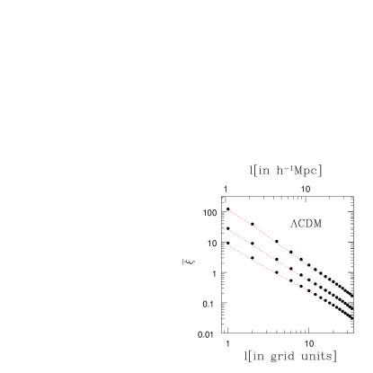
We have used the freely available intermediate scale $\Lambda$CDM N-body simulation from Virgo Consortium to test our analytical predictions. The cosmological parameters are largely compatible with recent observations, in particular we have $\Omega_{\rm m}=0.3$, $\Omega_{\Lambda}=0.7$, the Hubble constant is $H_{0}=70$ km/s/Mpc and $\sigma_{8}=0.9$. The box size is $L_{\rm box}=239.5h^{-1}$Mpc while the number of particles is $N_{p}=256^{3}$. We used three epochs at redshifts $z=0,1,2$ to compare our predictions with the simulations. We refer the reader to Jenkins et al. (1998) and Thomas et al. (1998) for more details about the simulations. The huge dynamic range studied by the VIRGO simulation provides an unique opportunity to probe the length scales from the quasi-linear regime up to the highly non-linear regime.

To confront analytical results with numerical simulations we have used a cubic $256^{3}$ grid. Then, we select cubic cells with volumes $l_{\rm grid}^{3}$, $8l_{\rm grid}^{3}$, $64l_{\rm grid}^{3}$ and $512l_{\rm grid}^{3}$. We compute the occupancy of each cell and the resulting count probability distribution. To increase the sampling random shifts were given to the 3D grid in orthogonal directions. This whole process was repeated several times to reach the number of cells which is required to probe low levels of probability. Note that an alternative method which is equivalent to infinite sampling is developed in Szapudi (1998). Next, we compare these numerical results with our analytical predictions. Note that our analytical pdfs apply to spherical cells (for which exact analytical results can be derived in the quasi-linear and rare-void limits). Therefore, we compare the pdf obtained from the N-body simulation for cubic cells of volume $l^{3}$ with our prediction for spherical cells of radius $R$ with the same volume: $l^{3}=4\pi R^{3}/3$. We shall see that we obtain a good agreement which shows that such a change in the shape of elementary cells has no strong influence. On the other hand, spurious effects such as the finite size of the simulations, shot noise and sampling errors need to be kept in mind while comparing analytical and simulation results.

Finite volume effects are due to the fluctuations of the underlying density perturbations on scales larger than the simulation box. Typically the tails of the count in cell (CIC) statistics are affected by the finite size of the catalogue. Such effects have been a very active area of research in recent past (Szapudi et al. 2000; Colombi et al. 2000) and much of the effort has been concentrated on trying to understand how they can be “corrected” so that meaningful statistical indicators can be constructed. Thus, it is known that the high-density far tail is very sensitive to the presence (or absence) of rare clusters in the catalogue. This yields random fluctuations before the pdf shows an abrupt cutoff corresponding to the densest cell in the finite catalog. This can also give a biased estimation for low order moments of the pdf such as the variance and the skewness. Of course, these problems worsen for smaller catalogs. In our studies we have used of the order of $10^{10}$ cells of various sizes. This means that we can construct the probabilities $P_{N}$ down to $10^{-10}$. We have avoided diluting the sample and we have used the full set of $256^{3}$ particles from the simulations in our construction of the pdf.

Discreetness effects are due to the sampling of the underlying continuous density field with finite point sets. However, techniques to subtract the Poisson shot noise from computed quantities are well known (see Munshi et al. 1999a for expressions regarding the shot noise contributions to underlying cumulants of smoothed field from central moments and factorial moments of cell count statistics, see also Szapudi & Szalay 1996). It is also possible to construct the analytical discrete pdf by convolving it with the Poisson sampling:

$${\cal P}_{N}=\int_{0}^{\infty}{\rm d}\rho_{R}\;{\cal P}(\rho_{R})\;\frac{(\rho_{R}\overline{N})^{N}}{N!}\;e^{-\rho_{R}\overline{N}},\;\;\;\overline{N}=\overline{n}V,$$ (38)

where $\overline{N}$ is the mean number of particles in a cell (and $\overline{n}$ is the mean number density of particles in the simulation box). However, in most of our cases we found that this correction is not required as theoretical predictions are already in good agreement with numerical data. On the other hand, since the lowest overdensity $\rho_{R}=N/\overline{N}$ that one can probe corresponds to $N=1$, which yields $\rho_{R}=1/\overline{N}$, larger cells which have a larger $\overline{N}$ probe farther into the low-density tail of the pdf. For the computation of low order moments we relied on factorial moments which can directly be related to low order moments of the underlying continuous field:

$$\sum_{N}\frac{N(N-1)\dots(N-p+1)}{\overline{N}^{p}}{\cal P}_{N}=\int_{0}^{\infty}{\rm d}\rho_{R}\;{\cal P}(\rho_{R})\;\rho_{R}^{p}.$$ (39)

For a complete discussion of generating functions, order by order expansions of low order factorial moments and their link with the normalized cumulants parameters $S_{N}$ see Munshi et al. (1999a).

Figure 2: The skewness $S_{3}$ computed from the simulations is compared with analytical predictions at redshifts $z=0,1,2$. Solid dots are results from numerical simulations whereas various lines are analytical predictions as labeled in the left panel. We display our interpolation eq.(32) (P), the EPT prediction from section 2.6.1 (EPT) and the lognormal approximation eq.(37) (Ln).

3.2 Variance and Skewness

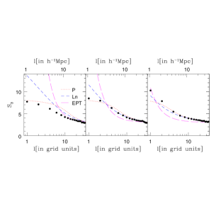
We first compare in Fig. 1 the variance $\overline{\xi}(R,z)$ we obtain from the procedure described in section 2.5 (following Peacock & Dodds 1996) with the numerical simulations. We can see that the agreement is quite good over all scales and redshifts we investigate in this paper. Therefore, this simple procedure appears to be sufficient for our purposes. Next, we display in Fig. 2 the predictions for the skewness $S_{3}(R,z)$ derived from our interpolation (32) between the quasi-linear limit and HEPT (Scoccimarro & Frieman 1999), from the EPT recalled in section 2.6.1 and from the lognormal approximation (37), as compared with N-body simulations. We can check that all three models are very close on quasi-linear scales and match the simulations. Note that for the lognormal model this is actually a coincidence because its skewness only agrees with the exact quasi-linear limit for $n=-1$ (compare eq.(37) with eq.(27)) and it happens that on the quasi-linear scales shown in Fig. 2 we have $n\simeq-1$ (as is usual for CDM power-spectra at such redshifts). On the other hand, we find that our interpolation and EPT prediction work rather well on non-linear scales at $z=1,2$ while the lognormal model shows a significant discrepancy. At $z=0$ our interpolation shows some deviation from the simulations but it fares much better than both EPT and the lognormal model. However, the comparison of the simulations at $z=0,1$ and $2$ suggests that on small scales finite resolution effects play a significant role (indeed, at fixed comoving scale one expects the skewness to grow with time, which is not the case in Fig. 2 below a few grid lengths). Therefore, some of the discrepancy between numerical simulations and the models could be due to such numerical effects.

3.3 Density pdf ${\cal P}(\rho_{R})$

Finally, we compare in Figs. 3-5 the pdfs ${\cal P}(\rho_{R})$ obtained from the different theoretical models with the results from N-body simulations. We display our model (26), EPT (33) and the lognormal model (36) at redshifts $z=0,1$ and $2$ and for four scales. We first plot $\rho_{R}^{2}{\cal P}(\rho_{R})$ (in logarithmic scales) which is the quantity of interest for most practical purposes. Indeed, $\rho_{R}^{2}{\cal P}(\rho_{R})$ is also the fraction of matter per logarithmic interval of overdensity ${\rm d}\ln(\rho_{R})$ at scale $R$. Moreover, it enables one to clearly see the evolution of the pdf into the non-linear regime. Thus, we see that while in the quasi-linear regime there is only one density scale: the mean density of the universe (that is $\rho_{R}=1$ in our units) and the pdf ${\cal P}(\rho_{R})$ tends to a simple Gaussian, as one goes deeper into the non-linear regime two density scales gradually appear. A low-density scale $\rho_{v}\ll 1$ marks the low-density cutoff of the pdf, below which one enters the rare-voids regime recalled in section 2.3. As seen in Valageas (2002b), this cutoff $\rho_{v}$ is given by:

$$\sigma\gg 1:\;\;\;\rho_{v}=\sigma(R)^{-6/(1-n)}\ll 1,$$ (40)

and the pdf ${\cal P}(\rho_{R})$ shows the modified exponential falloff:

$$\rho_{R}\ll\rho_{v}:\;\;\;{\cal P}(\rho_{R})\sim e^{-9\rho_{R}^{-(1-n)/3}/(8\sigma^{2})}.$$ (41)

Note that in the quasi-linear regime (i.e. $\sigma\ll 1$) the low-density falloff of ${\cal P}(\rho_{R})$ is still given by eq.(49) but the density scale $\rho_{v}$ goes to unity. This part of the pdf is governed by the last term in eq.(26), that is by the behaviour (24). A second density scale $\rho_{h}$ which marks the high-density cutoff of the pdf ${\cal P}(\rho_{R})$ is simply given by the two-point correlation $\overline{\xi}$:

$$\overline{\xi}\gg 1:\;\;\;\rho_{h}=S_{3}\;\overline{\xi}=\frac{\langle\rho_{R}^{3}\rangle_{c}}{\langle\rho_{R}^{2}\rangle_{c}}\gg 1.$$ (42)

It corresponds to the typical overdensity within virialized halos at scale $R$ while higher densities are associated with rare massive objects. The reason why we defined $\rho_{h}$ in eq.(42) from the second and third cumulants of the density pdf is that they are the lowest order cumulants which are mostly sensitive to the high-density part of the pdf. Thus, we can see from the figures that the mean $\langle\rho_{R}\rangle=1$ probes the whole range $\rho_{v}<\rho_{R}<\rho_{h}$ and we can check that at small scales the cutoff $\rho_{h}$ can indeed be significantly higher than $\overline{\xi}$ (compare Fig. 3 with Fig. 1) following the growth of the skewness $S_{3}$. On the other hand, higher-order cumulants probe increasingly large and rare overdensities and exhibit higher uncertainties. As for the low-density cutoff $\rho_{v}$, the high-density cutoff $\rho_{h}$ goes to unity in the quasi-linear regime so that both density scales merge to the mean density of the universe.

Figure 3: Analytical and numerical probability distribution functions are plotted for various smoothing scales $l$ (in grid units) as indicated in each panel. Lines of various styles represent analytical predictions from various theoretical models as labeled in the upper left panel. We show our model (26) (P), the EPT prediction (33) (EPT) and the lognormal approximation (36) (Ln). Dark solid lines are the results from numerical simulations. We have plotted $\rho_{R}^{2}{\cal P}(\rho_{R})$ vs $\rho_{R}$ (on logarithmic scales) which shows clearly the evolution of the pdf into the non-linear regime.

Figure 4: Same as previous figure but for z=1.

Figure 5: Same as previous figure but for z=2.

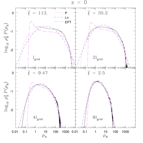
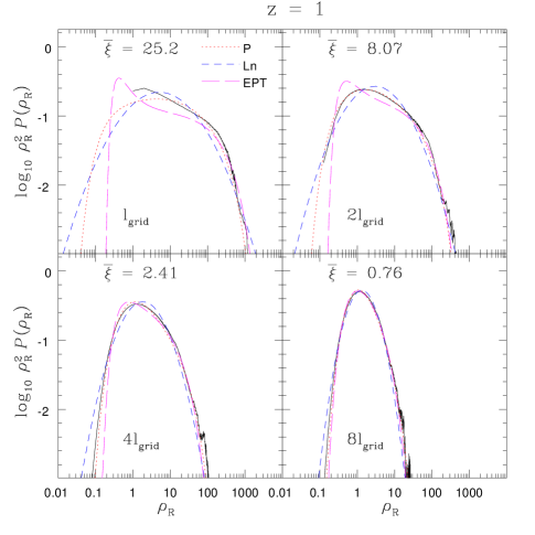
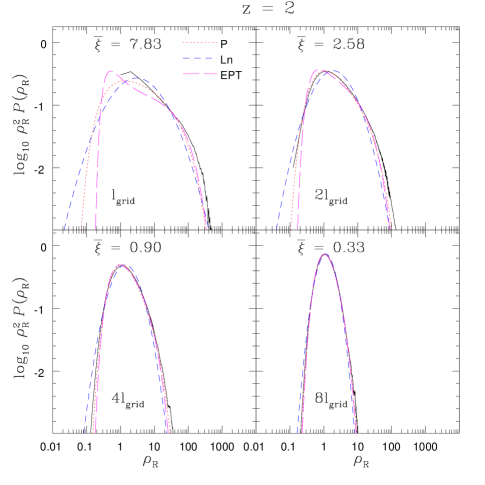
We can see in Figs. 3-5 that our simple model (26) agrees very well with the results from numerical simulations. Note moreover that our model has no free parameter beyond the variance (obtained from Peacock & Dodds 1996) and the skewness. The EPT model recalled in section 2.6.1 is also fully parameterized by $\overline{\xi}$ and $S_{3}$, but we can see that it shows significant discrepancies at small scales. This can be traced to its low-density behaviour which does not obey the properties (24) and (49). Indeed, it yields a much sharper low-density cutoff. In order to fulfill the normalization conditions (2) this implies a high peak at $\rho_{v}$ (to compensate for the smaller contributions from lower densities to the normalization $\langle 1\rangle=1$) and a lower plateau at intermediate densities (to compensate for this high peak at $\rho_{v}$ into the normalization $\langle\rho_{R}\rangle=1$). This failure to follow the evolution of the pdf into the non-linear regime comes from the fact that the EPT model (33) attempts to parameterize the evolution of rare underdensities and overdensities in the same fashion. That is, both the small $\zeta$ ($\zeta\ll 1$) and large $\zeta$ ($\zeta\geq 1$) parts of the function $\tau(\zeta)$ are parameterized by the same parameter $n_{\rm eff}$. In particular, if the stable-clustering Ansatz were valid (that is $S_{3}$ goes to a constant with time in the non-linear regime at fixed physical scale) the function $\tau(\zeta)$ from EPT would become constant. However, it is clear that this would miss the physics at work at low densities. Indeed, even though high-densities are governed by virialization processes which might stabilize high-density peaks observed in physical units, rare voids are governed by different phenomena and keep expanding faster than the mean universe. This is captured by the last term in our model (26) which shows the explicit time dependence $\overline{\xi}/\sigma^{2}$. This point is further discussed in section 3.6.3 in Valageas (2002b). Note that neither our model nor EPT assume that the stable-clustering Ansatz is valid but this discussion enables one to clearly see that rare underdensities and overdensities require distinct treatments.

The simple lognormal model shows a smooth parabolic-like shape in the scales used in Figs. 3-5 (actually $\log[\rho_{R}{\cal P}(\rho_{R})]$ would give an exact parabola over $\log\rho_{R}$) and it might appear to work better than EPT. However, we can see that our model (26) provides significantly better results as compared with numerical simulations. Indeed, the lognormal model yields low-density and high-density falloffs which are clearly too shallow and it does not follow very well the flat plateau in-between $\rho_{v}$ and $\rho_{h}$ because of its parabolic shape (the curvature is too high). The rather good success of our simple model (26) is due to its correct description of the low-density cutoff (as compared with EPT) and the normalization constraints (2). Indeed, the rare-void limit (24) together with the normalization $\langle 1\rangle=1$ set the location and the height of the low-density cutoff ${\cal P}(\rho_{v})$ (as well as lower densities). Next, the normalizations $\langle\rho_{R}^{2}\rangle_{c}=\overline{\xi}$ and $\langle\rho_{R}^{3}\rangle_{c}=S_{3}\overline{\xi}^{2}$ set the location and the height of the high-density cutoff ${\cal P}(\rho_{h})$ (see eq.(42)). Finally, the normalization $\langle\rho_{R}\rangle=1$ provides a further constraint on the pdf ${\cal P}(\rho_{R})$ over the whole range $\rho_{v}<\rho_{R}<\rho_{h}$. All these conditions are sufficient to provide a tight constraint onto the pdf ${\cal P}(\rho_{R})$ at densities $\rho_{R}<\rho_{h}$. This property is obviously a direct consequence of the weak dependency of the functions $\tau(\zeta)$ and $\varphi(y)$ onto additional free parameters discussed in appendix B once all constraints (23)-(25) are taken into account.

It might be possible to have a significantly different pdf ${\cal P}(\rho_{R})$ while satisfying the constraints (23)-(25) if we allow large oscillations in the intermediate range $\rho_{v}<\rho_{R}<\rho_{h}$. However, this would require a rather contrived model and Figs. 3-5 show that results from N-body simulations do not exhibit such peculiar behaviour. On the contrary, although the numerical simulations may not go sufficiently far into the non-linear regime to draw definite conclusions, it seems that no intermediate density scale shows up in the range $\rho_{v}<\rho_{R}<\rho_{h}$ and the pdf exhibits a smooth power-law behaviour over this range. In this sense, the outcome of gravitational clustering appears quite simple. Therefore, we can conclude that our model is very robust over the whole range $\rho_{R}<\rho_{h}$. Moreover, its prediction for ${\cal P}(\rho_{R})$ is the simplest one which can be made consistent with all known constraints.

Any deviation from our result over this range (in fact over $\rho_{v}<\rho_{R}<\rho_{h}$ since lower densities are known from section 2.3) would require additional parameters which would for instance introduce new density scales. An alternative possibility would have been a bimodal distribution. For instance, in a fashion similar to the behaviour shown by EPT in Fig.3, one could have imagined keeping the only two characteristic density scales $\rho_{v}$ and $\rho_{h}$ but having a specific power-law in the intermediate range which only connects smoothly to one extremity (for instance $\rho_{h}$) while the matching at the other hand (then $\rho_{v}$) involves a sharp transition. Another possibility would have been two distinct power-laws attached to each boundary $(\rho_{v},\rho_{h})$ which match in-between. It is not clear whether such behaviours could have been ruled out a priori. However, one may argue in this direction as follows. If we assume that the stable clustering Ansatz is valid, virialized objects are frozen in physical coordinates so that the high-density part of the pdf remains constant. Then, the intermediate power-law range only grows towards underdensities as increasingly underdense and extreme voids (as measured in the initial conditions) fill the whole volume and see their fast expansion stopped as they join. In this process, the matter at their boundaries forms filaments and virialized objects which become part of the matter described by the power-law regime while the mass associated with rare underdensities below $\rho_{v}$ keeps declining. Then, since at the beginning of this process the two density scales $\rho_{v}$ and $\rho_{h}$ coincide and the process repeats itself identically with time it is natural to expect the build-up of a unique power-law regime which smoothly connects both end-points $(\rho_{v},\rho_{h})$ (while a double power-law could have been expected if the matter in this range would originate both from $\rho_{v}$ and $\rho_{h}$, the flux from one extremity increasing as one gets closer). In practice, we do not expect such a stable clustering Ansatz to be valid, as moderate overdensities experience mergings and tidal effects. Nevertheless, the scale-free nature of gravity and the approximate self-similarity of the process, which starts from a unique origin ($\rho_{v}=\rho_{h}$), could still be the source of the simple behaviour seen in Figs. 3-5.

We must point out that this intermediate density range actually corresponds to the part which is most difficult to follow from a Lagrangian point of view. Indeed, it covers a wide range of objects (about three orders of magnitude over the density in the upper panels of Fig. 3), from low-density filaments which surround large voids up to typical virialized halos. The common property of these objects is that they have undergone strong interactions with the neighbouring density fluctuations and strong mergings. This makes it difficult for simple Lagrangian mappings (which attempt to map the linear density contrast $\delta_{L}$ to the actual non-linear density contrast $\delta$, possibly with some scatter) to model this density range. It is clear that our approach is completely different from this point of view as we do not try to identify non-linear density fluctuations from the linear density field on a one-to-one basis. On the contrary, we directly focus on the pdf ${\cal P}(\rho_{R})$, which is a statistical quantity, and we try to build a simple model which satisfies all known constraints. As seen above, it appears that this is actually sufficient to derive the pdf ${\cal P}(\rho_{R})$ over this density range up to a good accuracy. As noticed above, the reason for this pleasant result is that the intricate merging process which “shuffles” the matter associated with these typical density fluctuations does not bring about new scales and it yields a simple power-law behaviour in-between the low and high density cutoffs $\rho_{v}$ and $\rho_{h}$. Therefore, while the gravitational dynamics of these individual objects is extremely complex (they may even lose their identity through mergings or disruptions) the statistical outcome is very simple. This suggests that the appropriate method to investigate this system in a theoretical and rigorous manner from the equations of motion should rely on a statistical analysis.

On the other hand, we must point out that the very high-density regime $\rho_{R}\gg\rho_{h}$ is not constrained by the conditions (2) which allowed us to obtain ${\cal P}(\rho_{R})$ for $\rho_{R}<\rho_{h}$ with a good accuracy. As recalled in eq.(43), our model usually yields a singularity $y_{s}<0$ for the generating function $\varphi(y)$ (at least for $n<0$) which translates into a simple exponential cutoff for the high-density tail of ${\cal P}(\rho_{R})$, see eq.(44). Nevertheless, we must note that this behaviour should not be taken at face value and the very high-density tail could exhibit a different shape. As seen in Valageas (2002a) (section 3.6), this is actually the case in the quasi-linear limit where the singularity $y_{s}$ is somewhat spurious and one must follow a second branch of $\varphi(y)$ beyond $y_{s}$ which yields a high-density tail ${\cal P}(\rho_{R})\sim e^{-\rho_{R}^{(n+3)/3}/\sigma^{2}}$ which is shallower than a simple exponential for $n<0$. As discussed in Valageas (2002b) one can expect a similar behaviour at very high densities in the non-linear regime. However, at the scales and redshifts shown in Figs. 3-5 it appears that our model works reasonably well up to the highest densities probed by the numerical simulations and even higher densities are probably too rare to be of practical interest. On the other hand, in the quasi-linear regime our model goes to the exact quasi-linear limit (like EPT). As seen in Valageas (2002a), in this regime too the far tail where the deviation from the simple exponential cutoff discussed above could be seen corresponds to very rare events which are usually irrelevant.

Figure 6: Analytical and numerical probability distribution functions are plotted for various smoothing scales $l$ (in grid units) as indicated in each panel, over logarithmic scales. Lines of various styles represent analytical predictions from various theoretical models, while the numerical data is shown by dark solid lines, as in Fig. 3.

Figure 7: Same as previous figure but for z=1.

Figure 8: Same as previous figure but for z=2.

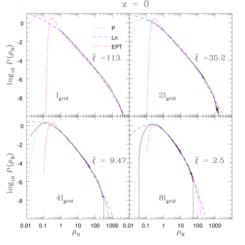
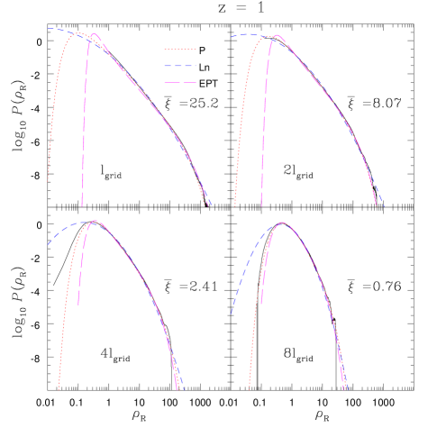
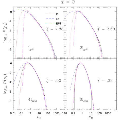
Finally, we show for completeness in Figs. 6-8 the pdf ${\cal P}(\rho_{R})$ from the various theoretical models and the N-body simulations. This emphasizes the low-density cutoff $\rho_{v}$ but the high-density cutoff $\rho_{h}$ is blurred by the huge vertical scale and cannot be easily distinguished from the intermediate power-law part. Of course, as in Figs. 3-5 we can check that our model (26) works best, while EPT yields too sharp a low-density cutoff at a larger density and the lognormal model gives too shallow a cutoff at a smaller density.

4 Conclusion

Thus, in this paper we have presented a new model to describe the evolution of the density probability distribution function ${\cal P}(\rho_{R})$. This allows us to follow the dynamics of gravitational clustering on cosmological scales from the linear regime up to the highly non-linear regime. Taking advantage of the known rigorous results which have been obtained in the quasi-linear limit and the rare underdense limit, we have built the simplest model which satisfies both these constraints as well as normalization conditions. Our model is fully parameterized by the non-linear variance and the skewness. Using standard estimates for these two quantities we have shown that our predictions match N-body simulations over the scales and redshifts of interest. Moreover, we have found that our model works significantly better than previous approximations (EPT and the lognormal).

We have explained that this success is due to two properties: i) the correct handling by our model of the rare void limit and ii) the simple statistical outcome of gravitational clustering over the range spanned by typical fluctuations. Indeed, following previous works (e.g., Balian & Schaeffer 1989, Colombi et al. 1997, Valageas 1998,1999) we have checked that in the non-linear regime two distinct density scales appear (which merge to the mean density of the universe $\overline{\rho}$ in the linear regime): a low density cutoff $\rho_{v}\ll\overline{\rho}$ and a high-density cutoff $\rho_{h}\gg\overline{\rho}$. The low density cutoff $\rho_{v}$ marks the transition to rare voids which keep expanding faster than the Hubble flow while the high density cutoff $\rho_{h}$ marks the transition to rare overdensities. The intermediate range $\rho_{v}<\rho_{R}<\rho_{h}$ corresponds to typical density fluctuations which have undergone mergings and tidal disruptions and spans a large variety of objects: from filaments surrounding large voids to moderate virialized halos. These structures cannot be followed by Lagrangian approaches since they have no well defined identities (because of mergings and disruptions) but it appears that the statistical outcome of this intricate gravitational dynamics is quite simple: the pdf obtained from numerical simulations exhibits a simple power-law behaviour over the whole range $\rho_{v}<\rho_{R}<\rho_{h}$ (i.e. no additional density scale appears). Then, this simple behaviour together with the rare-void limit and the normalization conditions provide a tight constraint on the pdf ${\cal P}(\rho_{R})$ over $\rho_{R}<\rho_{h}$ which can thus be predicted with a good accuracy. This also explains why it is possible to build a satisfactory model using only $\overline{\xi}$ and $S_{3}$. As described in section 3.3, these two quantities provide the location $\rho_{h}$ (see eq.(42)) and the height ${\cal P}(\rho_{h})$ of the high-density cutoff. Then, a simple power-law matching to the low-density cutoff $\rho_{v}$ (whose location and height are explicitly known as a function of $\sigma^{2}$) allows a complete description at all densities below (and also of the order of) $\rho_{h}$.

On the other hand, we have noticed that there are no rigorous results for the very high-density limit $\rho_{R}\gg\rho_{h}$ so that our model should be viewed with some caution in this regime. In particular, although our simple model usually yields an exponential tail at high densities we explained that one could expect a more general shape (the exponential of some power-law) as discussed in Valageas (2002b). If this high-density falloff were sharper than exponential it could be handled within our framework in a straightforward way by modifying the large-$\zeta$ part of the function $\tau(\zeta)$ we used in eq.(26) and making sure it yields no singularity. By contrast, if this high-density cutoff were shallower than exponential it would require a more important modification (see also Valageas 2002a for a similar case). A possible way to do so would be to consider the pdf and the cumulant generating function associated with the logarithm of the density $\ln\rho_{R}$ rather than the density $\rho_{R}$ itself. Here we may note that going to higher orders over $S_{p}$ (i.e. adding further constraints to (2) by including higher-order moments) does not appear to us to be the most promising way to improve this model. Indeed, it would add some further parameters which are not accurately known without ensuring that the large density limit is correct. In our view, one would rather like to derive the large-density behaviour of the pdf ${\cal P}(\rho_{R})$, or of the generating function $\tau(\zeta)$, and build a simple model for $\tau(\zeta)$ which recovers this asymptotic behaviour (as we did for the underdense limit). Unfortunately, this behaviour has not been derived yet (although one might try a version of the Press-Schechter (1974) prescription coupled to the stable-clustering Ansatz or some halo model). As discussed above, in such a case it could be more convenient to work with $\ln\rho_{R}$.

However, we shall not explore this point further in this paper because we have found that our model works quite well over the scales and redshifts of interest. Moreover, the very high-density tail $\rho_{R}\gg\rho_{h}$ where such deviations might appear is beyond the reach of these simulations and it corresponds to very rare overdensities which should be irrelevant for most practical purposes. In particular, the robustness of our model discussed above for $\rho_{R}<\rho_{h}$ ensures that we obtain good predictions for density fluctuations which occupy most of the volume and contain most of the matter of the universe. Besides, we can note that the constraint provided by the skewness actually means that we correctly describe the near high-density tail.

Therefore, we expect that this simple model should be useful for cosmological studies which require a realistic estimate of the probability distribution ${\cal P}(\rho_{R})$, from rare voids up to rare overdensities and from the linear regime up to the highly non-linear regime. In fact, this model is probably the simplest one which can be built consistently with all known results. It also suggests that a theoretical study of gravitational clustering on non-linear cosmological scales should rely on a statistical analysis rather than a detailed Lagrangian approach, as the properties of the system seem to be much simpler within a statistical perspective. However, such an analysis still remains to be done.

Finally, although we have focused on the one-point pdf in this paper, it is possible to extend our approach to analyze the bias associated with overdense cells and the detailed description of their multivariate distribution. A detailed analysis in line with Munshi et al. (1999b) and Bernardeau & Schaeffer (1999) will be presented elsewhere.

Appendix A Numerical implementation

Figure 9: The integration path over the complex $y-$plane used to compute the pdf ${\cal P}(\rho_{R})$ from eq.(45). We show the paths obtained at $z=0$ and at the scale $l=4l_{\rm grid}$ for $\rho_{R}=100,10$ and $5$ (this corresponds to the lower left panels in Figs. 3,6).

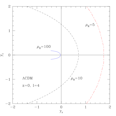
We have described in section 2 two models which yield the pdf ${\cal P}(\rho_{R})$ through its cumulant generating function $\varphi(y)$, the latter being determined through the implicit system (21)-(22). We explain in more details here how to compute numerically ${\cal P}(\rho_{R})$ within this framework. As is well-known, in the context of large scale structures the functions $\tau(\zeta)$ which appear in the implicit system (21)-(22) usually yield a singularity $y_{s}$ on the negative real axis for $\varphi(y)$ because the function $\tau(y)$ is bivaluate (e.g., Bernardeau & Schaeffer 1992, Bernardeau 1992, Valageas 2002a). This means that the parametric representation (21)-(22) for $\varphi(y)$ yields two branches (obtained for $\tau>\tau_{s}$ and $\tau<\tau_{s}$) which join at $y_{s}$, as seen for instance in Figs. 3-5 in Valageas (2002a) (see also Figs. 10-11 below). From the definition (3)-(5) of $\varphi(y)$, the branch of interest is the one which runs through $(y=0,\varphi=0)$ and $(\zeta=1,\tau=0)$, where we have the Taylor expansion $\varphi(y)=y-y^{2}/2+..$ (as we noticed below eq.(18) the linear term $y$ is usually removed in studies which focus on the quasi-linear regime by working with $\delta_{R}$ rather than $\rho_{R}$). As explained in Valageas (2002a), the non-perturbative steepest-descent approach shows that in the quasi-linear limit the second branch of $\varphi(y)$ is actually relevant as it governs the high-density tail of the pdf ${\cal P}(\rho_{R})$. However, for our present purposes it is irrelevant because our perspective is quite different. In this paper we do not compute ${\cal P}(\rho_{R})$ from the equations of motion, we merely build a phenomenological model for the pdf. Hence we actually define $\varphi(y)$ from the implicit system (21)-(22) so that the singularity $y_{s}$ is no longer an artifact but an element of the definition of $\varphi(y)$. As described in Colombi et al. (1997), one obtains from eqs.(21)-(22) the behaviour of $\varphi(y)$ near its singularity as:

$$y\geq y_{s}:\;\varphi(y)=\varphi_{s}+r_{s}(y-y_{s})+a_{s}(y-y_{s})^{3/2}+..,$$ (43)

which implies through the inverse Laplace transform (6) the high-density behaviour:

$$\rho_{R}\gg 1+\overline{\xi}:\;\;{\cal P}(\rho_{R})\propto\rho_{R}^{-5/2}\;e^{-|y_{s}|\rho_{R}/\overline{\xi}}.$$ (44)

In practice, we must ensure that the numerical computation of the inverse Laplace transform (6) does not cross the branch cut $y<y_{s}$. Moreover, as explained in Colombi et al. (1997), it is important to choose the integration path in the complex $y$-plane such that the argument of the exponential in eq.(6) is real, which avoids oscillations and ensures a fast convergence of the integral. To do so, one starts on the real axis at $y=y_{c}$ where $y_{c}$ is the saddle-point of the exponent (the path is symmetric with respect to the real axis). However, as recalled above we must not cross the real axis below $y_{s}$, hence for $y_{c}<y_{s}$ one usually starts the integration from $y_{s}$ (e.g., Colombi et al. 1997, Munshi et al. 2004). However, this procedure is not fully satisfactory, especially in the highly non-linear regime. We found that it is more efficient to first perform two integrations by parts in eq.(6) which yields:

$${\cal P}(\rho_{R})=\frac{1}{\rho_{R}^{2}}\int_{-i\infty}^{+i\infty}\frac{{\rm d}y}{2\pi i}\;e^{[\rho_{R}y-\varphi+\overline{\xi}\ln(\varphi^{\prime 2}/\overline{\xi}-\varphi^{\prime\prime})]/\overline{\xi}}.$$ (45)

Then, the saddle-point is given by:

$$\rho_{R}=\varphi^{\prime}-\overline{\xi}\;\frac{\varphi^{\prime\prime\prime}-2\varphi^{\prime}\varphi^{\prime\prime}/\overline{\xi}}{\varphi^{\prime\prime}-\varphi^{\prime 2}/\overline{\xi}}\;\;\;\;\mbox{at}\;\;\;\;y_{c}.$$ (46)

Now the saddle-point $y_{c}$ “feels” the existence of the singularity $y_{s}$ and always obeys $y_{c}>y_{s}$. Indeed, from eq.(43) one can easily see that we have the asymptotic behaviour:

$$\rho_{R}\rightarrow\infty:\;\;y_{c}-y_{s}\sim\frac{\overline{\xi}}{\rho_{R}},$$ (47)

which automatically gives the high-density behaviour (44) from eq.(45). Note that a single integration by parts would also give $y_{c}>y_{s}$ but it would yield the spurious scaling $(y_{c}-y_{s})\sim(\overline{\xi}/\rho_{R})^{2}$ which would naively imply a power-law prefactor $\rho_{R}^{-3}$ instead of $\rho_{R}^{-5/2}$ in eq.(44). Of course, in principle any procedure (with none or several integrations by parts) must give the same results but those which are not well-suited to the singular behaviour (43) imply a higher computational cost for a given accuracy. On the other hand, the underdense regime ($\rho_{R}\rightarrow 0$ and $y_{c}\rightarrow+\infty$) shows no particular problem. As seen in Valageas (2002b) the exact asymptotic behaviour (19), which is verified by our model, leads to:

$$y\rightarrow+\infty:\;\;\varphi(y)\propto y^{(1-n)/(4-n)},$$ (48)

and:

$$\rho_{R}\rightarrow 0:\;\;{\cal P}(\rho_{R})\propto\rho_{R}^{(n-13)/6}\;e^{-9\rho_{R}^{-(1-n)/3}/(8\sigma^{2})}.$$ (49)

The numerical factor $9/8$ in eq.(49) was changed to $(27/20)^{2}/2$ in Valageas (2002b) where we considered a critical-density universe. As noticed in section 2, this dependence on cosmology can actually be neglected. Moreover, one easily see from eq.(6) that the asymptotic behaviour (48) implies ${\cal P}(\rho_{R})=0$ for $\rho_{R}<0$ (by pushing the integration path over $y$ to $\Re(y)\rightarrow+\infty$).

We show in Fig.9 the integration paths over the complex $y-$plane used to compute the pdf ${\cal P}(\rho_{R})$ from eq.(45), at $z=0$ and at the scale $l=4l_{\rm grid}$, for $\rho_{R}=100,10$ and $5$, which corresponds to the lower left panels in Figs. 3,6. For lower densities the integration path crosses the real axis at a larger $y_{c}$ (with $y_{c}\rightarrow+\infty$ for $\rho_{R}\rightarrow 0$) while for high densities it gets closer to the singularity $y_{s}<0$ (with $y_{c}\rightarrow y_{s}^{+}$ for $\rho_{R}\rightarrow\infty$, see eq.(47)) and it bends more closely along the branch cut (i.e. the negative real axis with $y<y_{s}$). Moreover, for the same relative accuracy, for a higher density one only needs to integrate over a shorter length on $y$ but with smaller steps.

Appendix B Robustness of the model

Figure 10: The function $y(\zeta)$ obtained at $z=0$ and at the scale $l=l_{\rm grid}$ (this corresponds to the upper left panels in Figs. 3,6). We show the results derived with $d=1$ (dashed line), $d=2$ (solid line) and $d=3$ (dotted line).

Figure 11: The cumulant generating function $\varphi(y)$ obtained at $z=0$ and at the scale $l=l_{\rm grid}$ (this corresponds to the upper left panels in Figs. 3,6). We show the results derived with $d=1$ (dashed line), $d=2$ (solid line) and $d=3$ (dotted line). We also plot $\varphi(y)$ for the lognormal model (36) (dot-dashed curve for $y\geq 0$).

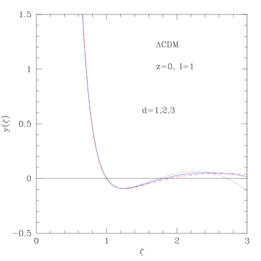
In the simple expression (26) which defines our model, the last two terms are set by the quasi-linear limit and the low-density regime. However, the first two terms $a+b\zeta^{2}$ are somewhat arbitrary. Indeed, although their normalization is given by the constraints (25) we could have used other powers or functions. Thus, we could replace for instance $a+b\zeta^{2}$ by $a+b\zeta^{d}$ with any $d$ larger than $(n-1)/6$ (so that the low-density limit $\zeta\rightarrow 0$ remains correct). However, we have checked through numerical computations that the dependence of our results on this free parameter is actually negligible: the different curves we obtain for the pdf ${\cal P}(\rho_{R})$ are almost indistinguishable in all cases described in section 3, where we compare our results with N-body simulations. The reason for this independence on the parameter $d$ can be seen in Fig. 10, where we display the function $y(\zeta)$ obtained from eqs.(22),(26). We consider the scale $l=l_{\rm grid}$ (with $l_{\rm grid}$ being the grid unit of the simulations) and the redshift $z=0$, which is the most non-linear case (upper left panels in Figs. 3,6). We show in Fig. 10 the functions $y(\zeta)$ obtained for a parameter $d=1,2$ and $3$, the exponent $d=2$ being our fiducial model as written in eq.(26). Then, we see that all three curves $y(\zeta)$ are very close for $\zeta\la 1.5$. Indeed, the low-density part $\zeta<1$ goes to the rare-void limit described in section 2.3 and eq.(24) while the behaviour near $\zeta=1$ is constrained by (25). Next, we note that at $\zeta_{s}\simeq 1.3$ the function $y(\zeta)$ reaches a minimum. This translates into a singularity for $\varphi(y)$ since this means that $\zeta(y)$ and $\varphi(y)$ become bivaluate. More precisely, near this minimum we have $y-y_{s}\sim(\zeta-\zeta_{s})^{2}$ which yields $\zeta-\zeta_{s}\sim\pm|y-y_{s}|^{1/2}$ and the power $3/2$ in eq.(43) for $\varphi(y)$. Then, as discussed in section A, this gives several branches for $\varphi(y)$ and we must only keep the one which connects to the underdense regime, which corresponds to the part of $y(\zeta)$ with $\zeta<\zeta_{s}$. Since this singularity $\zeta_{s}$ is close to $1$ it is strongly constrained by eqs.(25) and the dependence on the parameter $d$ of the function $\tau(\zeta)$ (or $y(\zeta)$) is very weak over this range $\zeta<\zeta_{s}$.

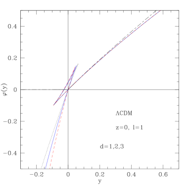
This behaviour can also be seen from Fig. 11 where we display the cumulant generating function $\varphi(y)$ for the same cases as in Fig. 10. The relevant branch of $\varphi(y)$ which defines the pdf ${\cal P}(\rho_{R})$ is the one which runs through the origin $y=0$ and extends up to $y\rightarrow+\infty$ (extreme underdensities). Again, we see that the three curves obtained for $d=1,2$ and $3$ are indistinguishable over this branch. By contrast, one can see some deviations appear as one follows the other branches down to $y\rightarrow-\infty$ (which corresponds here to $\zeta\rightarrow+\infty$) but they have no signification for the pdf ${\cal P}(\rho_{R})$.

For completeness, we also display in Fig. 11 the generating function $\varphi(y)$ obtained for the lognormal model (36). It is restricted to $y\geq 0$ since the integral (5) diverges for $y<0$ because the high-density tail of the lognormal decreases more slowly than a simple exponential. In other words, we now have $y_{s}=0$. On the other hand, at very large $y$ the lognormal approximation yields $\varphi(y)\sim\ln^{2}y$ contrary to the power-law (48). Thus, one can already see on $\varphi(y)$ the differences between various models for ${\cal P}(\rho_{R})$.

References

- [1] Balian R., Schaeffer R., 1989, 220, 1
- [2] Bernardeau F., 1992, ApJ, 392, 1
- [3] Bernardeau F., 1994a, A&A, 291, 697
- [4] Bernardeau F., 1994b, ApJ, 427, 51
- [5] Bernardeau F., Schaeffer R., 1992, A&A, 255, 1
- [6] Bernardeau F., Kofman L., 1995, ApJ, 443, 479
- [7] Bernardeau F., Schaeffer R., 1999, A&A, 349, 697
- [8] Coles P., Jones B., 1991, MNRAS, 248, 1
- [9] Colombi S., Bernardeau F., Bouchet F.R., Hernquist L., 1997, MNRAS, 287, 241
- [10] Colombi S., Szapudi I., Jenkins A., Colberg J., 2000, MNRAS, 313, 711C
- [11] Fosalba P., Gaztanaga E., 1998, MNRAS, 301, 503
- [12] Jenkins A. et al., 1998, ApJ, 499, 20-40
- [13] Kayo I., Taruya A., Suto Y., 2001, ApJ, 561, 22
- [14] Munshi D., Sahni S., Starobinsky A.A., 1994, ApJ, 436, 517
- [15] Munshi D., Bernardeau F., Melott A.L., Schaeffer R., 1999a, MNRAS, 303, 433
- [16] Munshi D., Coles P., Melott A.L., 1999b, MNRAS, 307, 387
- [17] Munshi D., Valageas P., Barber A.J., 2004, MNRAS, 350, 77
- [18] Peacock J.A., Dodds S.J., 1996, MNRAS, 280, L19
- [19] Peebles P.J.E., 1980, The large scale structure of the universe (Princeton University Press)
- [20] Press W., Schechter P., 1974, ApJ, 187, 425
- [21] Protogeros Z.A.M., Scherrer R.J., 1997, MNRAS, 284, 425
- [22] Scoccimarro R., Couchman H.M.P., 2001, MNRAS, 325, 1312
- [23] Scoccimarro R., Frieman J.A., 1999, ApJ, 520, 35
- [24] Smith R. E., Peacock J. A., Jenkins A., White S. D. M., Frenk C. S., Pearce F. R., Thomas P. A., Efstathiou G., Couchman H. M. P, 2003, MNRAS, 341, 1311
- [25] Sheth R.K., 1998, MNRAS, 300, 1057
- [26] Szapudi I., 1998, ApJ, 497, 16
- [27] Szapudi I., Szalay A. S., 1996, ApJ, 459, 504
- [28] Szapudi I., Colombi S., Jenkins A., Colberg J., 2000, MNRAS, 313, 725S
- [29] Thomas P.A. et al., 1998, MNRAS, 296,1061
- [30] Valageas P., 1998, A&A, 337, 655
- [31] Valageas P., 1999, A&A, 347, 757
- [32] Valageas P., 2002a, A&A, 382, 412
- [33] Valageas P., 2002b, A&A, 382, 450
- [34] Valageas P., Lacey C., Schaeffer R., 2000, MNRAS, 311, 234