11email: eckart@ph1.uni-koeln.de 22institutetext: Center for Space Research, Massachusetts Institute of Technology, Cambridge, MA 02139-4307, USA
22email: fkb@space.mit.edu 33institutetext: Department of Physics and Astrometry, University of California Los Angeles, Los Angeles, CA 90095-1562, USA 44institutetext: Department of Astronomy and Astrophysics, Pennsylvania State University, University Park, PA 16802-6305, USA 55institutetext: Max Planck Institut für extraterrestrische Physik, Giessenbachstraße, 85748 Garching, Germany 66institutetext: Department of Astronomy and Radio Astronomy Laboratory, University of California at Berkeley, 601 Campbell Hall, Berkeley, CA 94720, USA
First Simultaneous NIR/X-ray Detection of a Flare from SgrA*
We report on the first simultaneous near-infrared/X-ray detection of the SgrA* counterpart which is associated with the massive 3–4106M⊙ black hole at the center of the Milky Way. The observations have been carried out using the NACO adaptive optics (AO) instrument at the European Southern Observatory’s Very Large Telescope111Based on observations at the Very Large Telescope (VLT) of the European Southern Observatory (ESO) on Paranal in Chile; Program: 271.B-5019(A). and the ACIS-I instrument aboard the Chandra X-ray Observatory. We also report on quasi-simultaneous observations at a wavelength of 3.4 mm using the Berkeley-Illinois-Maryland Association (BIMA) array. A flare was detected in the X-domain with an excess 2 - 8 keV luminosity of about 61033 erg/s. A fading flare of Sgr A* with 2 times the interim-quiescent flux was also detected at the beginning of the NIR observations, that overlapped with the fading part of the X-ray flare. Compared to 8-9 hours before the NIR/X-ray flare we detected a marginally significant increase in the millimeter flux density of Sgr A* during measurements about 7-9 hours afterwards. We find that the flaring state can be conveniently explained with a synchrotron self-Compton model involving up-scattered sub-millimeter photons from a compact source component, possibly with modest bulk relativistic motion. The size of that component is assumed to be of the order of a few times the Schwarzschild radius. The overall spectral indices () of both states are quite comparable with a value of 1.3. Since the interim-quiescent X-ray emission is spatially extended, the spectral index for the interim-quiescent state is probably only a lower limit for the compact source Sgr A*. A conservative estimate of the upper limit of the time lag between the ends of the NIR and X-ray flare is of the order of 15 minutes.
Key Words.:
Sagittarius A* – Black Hole – Galactic Center – Flare – X-ray – Near Infrared1 Introduction
Over the last decades, evidence has been accumulating that most quiet galaxies harbor a massive black hole (MBH) at their centers. Especially in the case of the center of our Galaxy, progress could be made through the investigation of the dynamics of stars (Eckart & Genzel 1996, Genzel et al. 1997, 2000, Ghez et al. 1998, 2000, 2003a, 2003b, Eckart et al. 2002, Schödel et al. 2002, 2003). Located at a distance of only 8 kpc from the solar system (Reid 1993, Eisenhauer et al. 2003), it allows detailed observations of stars at distances much less than 1 pc from the central black hole candidate, the compact radio source Sgr A*. Additional strong evidence for a massive black hole at the position of Sgr A* came from the observation of interim-quiescent and flare activity from that position both in the X-ray and recently in the near-infrared wavelength domain (Baganoff et al. 2001, 2003, Eckart et al. 2003, Porquet et al. 2003, Goldwurm et al. 2003, Genzel et al. 2003, Ghez et al. 2004). Throughout the paper we will use the term ’interim-quiescent’ (or IQ) for the apparently constant, low-level flux density states at any given observational epoch since current data cannot exclude flux density variations of that state on longer time scales (days to years). This is especially true for the more compact NIR source (Genzel et al. 2003, Ghez et al. 2004).
Simultaneous observations of SgrA* across different wavelength regimes are of high value, since they provide information on the emission mechanisms responsible for the radiation from the immediate vicinity of the central black hole. The first observations of SgrA* covering an X-ray flare simultaneously in the near-infrared using seeing limited exposures revealed only upper limits to the NIR flux density (Eckart et al. 2003). In section 2 of the present paper we report on the first successful simultaneous NIR/X-ray observations using adaptive optics. These observations were for the first time successful in detecting radiation from the SgrA* counterpart both in the NIR and the X-ray wavelength domain. A detailed statistical analysis that supports the simultaneous detection of a SgrA* flare event in the NIR and X-ray domain is given in section 3 of this paper. In section 2 we also describe the quasi-simultaneous mm-observations that were taken just before and after the NIR/X-ray observations. In section 4 we briefly discuss the flux densities and spectral indices we derived from the available data. Section 5 gives a first physical interpretation of the simultaneous detection of SgrA*. A short summary and discussion of the results is given in section 6.
2 Observations and Data Reduction
The Galactic Center stellar cluster was observed during Directors Discretionary Time on June 19, 2003, with the NAOS/CONICA adaptive optics system/NIR camera at the ESO VLT unit telescope 4. The loop of the AO was closed on the bright (K) supergiant IRS 7, located about north of Sgr A*. We used the KS-filter (, FWHM ). The detector integration time was 10 s, with two frames added online to final exposures of 20 s integration time. The visible seeing at zenith was around . The AO correction was stable, but of medium quality with an estimated Strehl ratio above most of the time. The correction improved during the course of the observations. The airmasses were all less than 1.1.
The individual exposures were sky subtracted, flat-fielded and corrected for bad pixels. We extracted PSFs for each of the images with StarFinder and used the extracted PSFs for a Lucy-Richardson deconvolution of all the images. After beam restoration with a Gaussian PSF of 60 mas FWHM, we extracted the flux of individual sources with aperture photometry. The stars W6, mK=14.30.2, W9, mK=13.70.2, and W11, mK=14.10.2, (Ott 2003) were used for the photometric calibration. These stars are located only about west of SgrA* and were contained in all the images. Under the favorable seeing conditions and small zenith angles photometric calibration with adaptive optics over such angular distances can usually be applied without problems. For precise relative photometry we used the stars S1, S2, and S8, all within of Sgr A* (see below). We repeated the photometric measurements with two different aperture sizes (26 and 39 mas) and took the average of these measurements as the source fluxes, with the errors given by the maximum deviation of the individual measurements from the average. We derived extinction corrected fluxes, assuming A (Genzel et al. 2003).
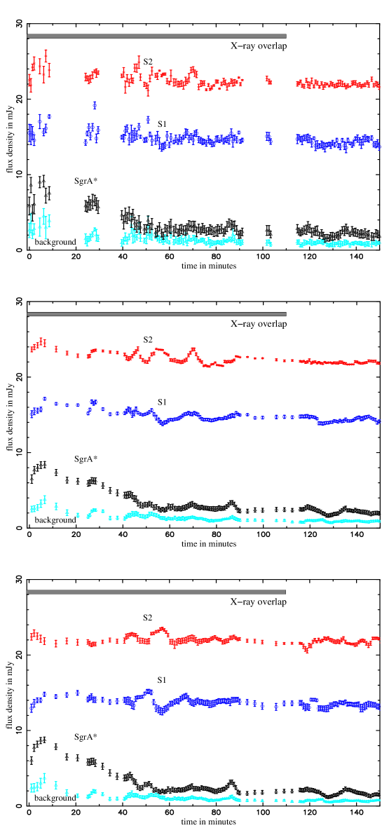
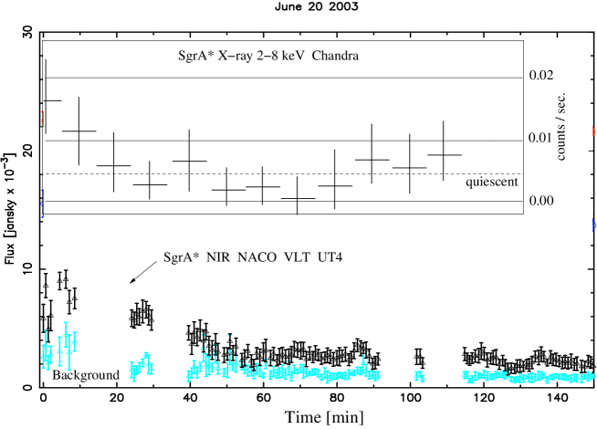
In the top panel of Figure 1 we show the light curves of Sgr A*, and of the two stars S1 and S2 (top curves: fluxes of S1 and S2 multiplied by a factor of ), that are located in its immediate vicinity. In order to estimate the background, we averaged aperture photometric measurements from six random locations within a region with no detectable source, about W of SgrA* (Figure 1, bottom light curve). For a better visualization of the flux variations of Sgr A* during the first 60 min, the middle panel of Figure 1 shows the same light curves of the upper panel after smoothing them with a sliding window that averages four measurements at a time. As can be seen in the middle panel of Figure 1, there appear still to be some correlated remnant flux variations. Therefore, we used the stars S1, S2, and S8 and could largely remove these variations by assuming a constant flux for these stars. The resulting light curves are shown in the lower panel of Figure 1.
The gaps in the measurements are due to AO reconfiguration or sky measurements. AO correction was poor during the first ten minutes of the observations. This is the reason for the larger error bars and the increased background level at the beginning of the light curves. In comparison to the light curves of the background, S1, and S2 (that are assumed to have a constant flux, of course), the flux of Sgr A* is clearly increased ( as can be seen in the lower, averaged plot) at the beginning of the observations and decreases until it reaches almost the background level.
Very close to the position of Sgr A* faint stellar sources can be detected when one averages individual images. We estimate that a possible systematic positive bias of the Sgr A* flux density due to these faint stars is of the order of to mJy. This is apparently less than the total measured IQ flux density (2 mJy) between 55 and 150 minutes.
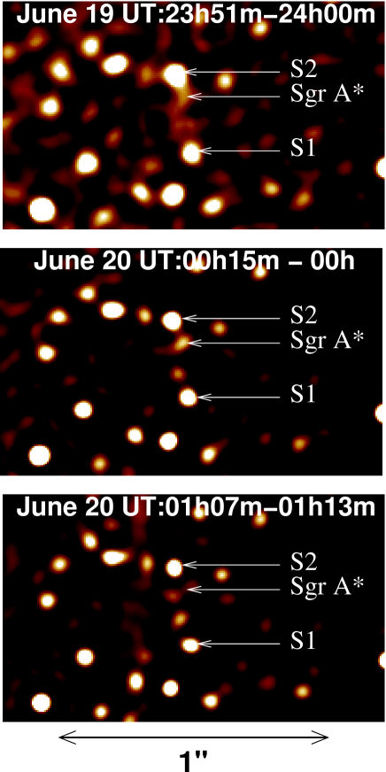
The flaring of Sgr A* can be seen in Figure 2. In the top panel we show the average of eight images at the beginning of the observations. The middle panel shows the average of eight images that were obtained about 25 min after the begin of the observations. Eight images about 80 min into the observations are averaged in the bottom panel. The VLT 8.2 m Unit Telescopes of the first image of each series are indicated in all the panels. All images resulted after Lucy-Richardson deconvolution and beam restoration. One can see how the AO correction improved between images 1 and 2. Sgr A* can be seen as a flaring source in the first two images and is not visible in the last image.
The offset of the flaring source at the position of SgrA* from the dynamical position of SgrA* - taking into account the orbit of S2 (Schödel et al. 2003) - is 62 mas in R.A. and 124 mas in Dec. and well within the values obtained for the previously detected flares of SgrA* (Ghez et al. 2004, Genzel et al. 2003). The deviation from the nominal position of Sgr A* is most probably due to the weakness of the flare and due to the proximity of faint stellar sources.
In parallel to the NIR observations, SgrA* was observed with Chandra using the imaging array of the Advanced CCD Imaging Spectrometer (ACIS-I; Weisskopf et al., 2002) for 25.1 ks on 19–20 June 2003 (UT). The start and stop times are listed in Table 2. The instrument was operated in timed exposure mode with detectors I0–3 turned on. The time between CCD frames was 3.141 s. The event data were telemetered in faint format.
We reduced and analyzed the data using CIAO v2.3222Chandra Interactive Analysis of Observations (CIAO), http://cxc.harvard.edu/ciao software with Chandra CALDB v2.22333http://cxc.harvard.edu/caldb. Following Baganoff et al. (2003), we reprocessed the level 1 data to remove the 0.25″ randomization of event positions applied during standard pipeline processing and to retain events flagged as possible cosmic-ray afterglows, since the strong diffuse emission in the Galactic Center causes the algorithm to flag a significant fraction of genuine X-rays. The data were filtered on the standard ASCA grades. The background was stable throughout the observation, and there were no gaps in the telemetry.
The X-ray and optical positions of three Tycho-2 sources were correlated (Høg 2000) to register the ACIS field on the Hipparcos coordinate frame to an accuracy of 0.10″ (on axis); then we measured the position of the X-ray source at Sgr A*. The X-ray position [J2000.0 = , J2000.0 = ] is consistent with the radio position of Sgr A* (Reid et al. 1999) to within ().
We extracted counts within radii of 0.5″, 1.0″, and
1.5″ around Sgr A* in the 2–8 keV band. Background counts
were extracted from an annulus around Sgr A* with inner and outer
radii of 2″ and 10″, respectively, excluding regions
around discrete sources and bright structures
(Baganoff et al. 2003). The mean count rates within each radius
are listed in Table 3. The background rates have been
scaled to the area of the source region. We note that the mean source
rate in the 1.5″ aperture is consistent with the mean quiescent
source rates from previous observations
(Baganoff et al. 2001, Baganoff et al. 2003).
The PSF encircled energy within each aperture increases from
for the smallest radius to for the
largest, while the estimated fraction of counts from the background
increases with radius from to . Thus, the
1.0″ aperture provides the best compromise between maximizing
source signal and rejecting background.
We observed Sgr A* at 3.4 mm wavelength with the
Berkeley-Illinois-Maryland Association (BIMA)
array (Welch et al. 1996) in its D configuration on 19 and 20 June 2003.
Observations on both days were performed identically over the LST
range 17.5 to 19.0 hours (07:47 to 09:17 UT on 19 June 2003).
These two observations occur approximately 9 hours before the start of
the Chandra observations and 4 hours after the end of the VLT
observations, respectively.
This is 8-9 hours before and 7-9 hours after the end of the flare
observed in the X-ray/NIR wavelength domain.
We observed the compact extragalactic source NRAO 530 (J1733-1303)
three times
during the course of each observation. For both sources, we
applied only the a priori amplitude calibration.
The D configuration is the most compact configuration, with
baseline lengths ranging from 1 to 9.5 kilolambda, corresponding to
a resolution of about 20 arcsec.
The substantial
confusion from free-free emission on these baselines makes estimates of
the absolute flux density and time variability during
these scans difficult.
Comparison with past longer baseline
observations allows us to determine
the contribution of the free-free emission and to estimate
the absolute flux density of Sgr A* to be Jy on 19 June
2003 (Bower et al. 2001).
We are able to determine the difference in flux density between
the two epochs with much greater precision by differencing the two
epochs. We find
a marginally significant increase in the flux density of Sgr A* from 19
June to 20 June of
%. The flux density of NRAO 530 changed by significantly
less,
%.
3 Variability Analysis
Figure 1 and Figure 2 show the clear detection of a decaying flare in the NIR emission of SgrA*. This flare is accompanied by an apparently simultaneous flare event in the X-ray domain (see Figures 1 and 3). The following analysis consolidates the significance of the X-ray flare and the correlation with the NIR flare event.
As a first step in our variability analysis of the X-ray data, we constructed binned light curves of the source intensity for each aperture using 10 minute bins, then we tested each curve against the null hypothesis of a constant count rate. The statistic and degrees of freedom for each fit are listed in Table 3. In each case, a constant count rate yielded an acceptable fit to the data; for such low count rates, however, analyses of binned light curves are not particularly sensitive tests for variability.
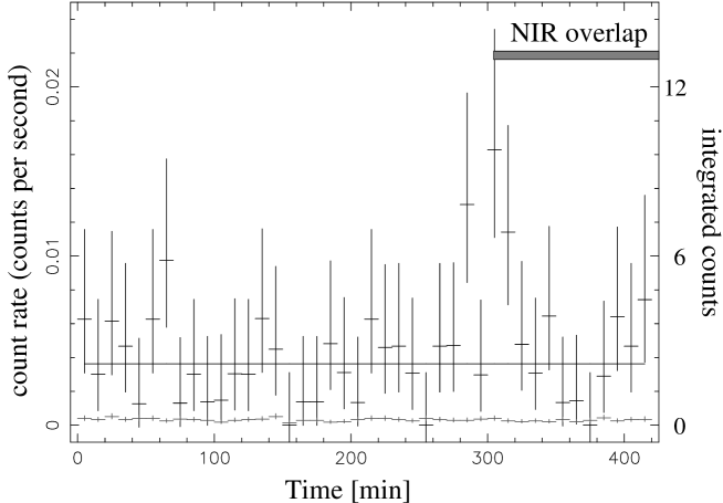
Figure 3 shows the source and background light curves for the 1.0″ aperture. We note that the three highest points are clustered within a 40 minute interval centered around 300 minutes after the start of the Chandra observation, and the first VLT/NACO image was taken 0.38 minutes before the midpoint of the highest X-ray data point. The NIR light curve in Figure 1 shows clearly that Sgr A* was in a flaring state at this time.
To investigate this further, we applied a standard Kolmogorov-Smirnov (K-S) test to the arrival times of the X-ray photons within each aperture. Multiple photons were occasionally detected in the same CCD frame. We corrected for this by redistributing their arrival times over the frame interval using uniform random deviates. The K-S test revealed no evidence for significant variability (see Table 4). The sensitivity of this test, however, depends on the location of the maximum deviation along the distribution. Press et al. (1992) present a variant of the K-S test called the Kuiper test that solves this problem by using the sum of the maximum deviations of the observed cumulative distribution above and below the theoretical distribution rather than the maximum absolute deviation used in the K-S test. The results of the Kuiper test are shown in Table 4. The evidence for variability in the 1.0″ and 1.5″ apertures, which contain a higher fraction of background counts from diffuse emission, was marginally significant: confidence; while the evidence for variability in the 0.5″ aperture was highly significant: 99.4% confidence. The results of the Kuiper test thus suggest that Sgr A* varied in X-rays; even so, it gives us no objective information about the location, duration, and amplitude of the variability.
A flexible method for obtaining such information is the Bayesian blocks algorithm of Scargle (1998), which uses the Poisson distribution and Bayesian statistics to partition an interval of data into piecewise constant segments or blocks. Each block is modeled as a Poisson process with constant intensity. A revised version (Scargle et al. 2004) of the original method incorporates an algorithm for finding the global, optimal partitioning of data on an interval (Jackson et al., 2003).
The algorithm uses a geometric prior of the form , where is the number of change points, is the prior probability distribution on the number of change points, and is an adjustable parameter (Scargle et al., 2003, 2004). Taking the logarithm of both sides yields the following contribution to the log-posterior: . This additive term in the fitness function penalizes more complex models; that is, models with more blocks. Setting corresponds to choosing a uniform prior, , where all values of are equally likely. The higher is set, the harder it becomes for the algorithm to add change points defining more blocks.
The value of can be converted into a prior odds ratio, , giving the ratio—before analyzing the data—of the probability that the source varied at all to the probability that it was constant. This would equal for an infinite geometric series, but can never be greater than the number of detected photons, so the actual form of the odds ratio is more complicated (J. D. Scargle 2003, private communication). In practice, however, the series converges rapidly for .
In Bayesian statistics, the posterior probability that the model is correct given the data is proportional to the product of the prior probability, expressing our knowledge or ignorance of the truth of the model before analyzing the data, and the likelihood function, which is the probability of the data given the model (Sivia 1996). As noted above, the prior odds ratio introduces a bias against more complex models. The preference of the data for the more complex model must be compelling enough to overcome the prior bias before the algorithm will introduce a new change point. In other words, the ratio of the likelihood functions for the data given the models must be greater than the inverse of the prior odds ratio.
We applied the global Bayesian blocks algorithm to a binned light curve of the total counts in the 1.0″ aperture using 157.052 second bins (i.e., 50 times the interval between CCD frames). Figure 5 shows the Bayesian blocks decomposition of the light curve obtained with , corresponding to a prior odds ratio of . Two change points were found 279.1 and 321.2 minutes into the observation indicating that Sgr A* flared in X-rays around midnight. Similar results were obtained for bin sizes ranging from 10 to 200 times the interval between CCD frames.
The mean count rate and start and stop times for the three blocks are presented in Table 5. The count rates during blocks 1 and 3 were fully consistent with each other. The mean rate for these two intervals combined was () counts s-1, whereas the mean rate during block 2 was counts s-1: a difference of counts s-1.
We performed Monte Carlo simulations to determine the posterior probability of obtaining a block with a rate greater than or equal to that of block 2. Using the mean rate over the entire observation (i.e., counts s-1), we generated 100,000 simulated Poisson data sets with each set having the same number of counts as the real data. We then binned the counts into light curves and ran the Bayesian blocks algorithm on each simulated light curve as before. The algorithm gave a false positive rate or posterior probability of , which is less than twice the prior odds ratio estimated above. Thus, the null hypothesis of a constant rate is rejected with 99.923% confidence, and we conclude that Sgr A* flared in X-rays for a period of about 42 minutes, which is characteristic of both the X-ray and NIR flares detected in previous observations (Baganoff et al., 2001, 2003; Goldwurm et al., 2003; Porquet et al., 2003; Eckart et al. 2003, Genzel et al., 2003; Ghez et al., 2004).
3.1 Properties of the Lightcurves
From linear fits to the data in the rising and decaying flanks of the X-ray and NIR flare including the measurement uncertainties (Figures 1 and 3) we can estimate the times at which the flare emission was negligible, i.e. equal to the IQ-state emission. The corresponding full width at zero power (FWZP) and start and stop times (see Table 1) compare well with the times of the change points and widths derived from the Bayesian blocks routine. They are earlier and later than the respective turn-on and turn-off change points. Also an estimate of the FWHM (Table 1) of the flare from Figure 3 is comparable to the flare duration derived from the Bayesian blocks analysis.
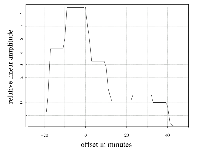
Further support for the detection of a simultaneous flare at NIR and X-ray wavelengths comes from a cross-correlation between the variability data obtained in both domains. The analysis was performed on the measured NIR lightcurve (Figure 1, upper panel) and on the X-ray data shown in Figure 3. A constant flux density contribution to SgrA* (see next section and Tab.1) was subtracted before the analysis. The cross-correlation was performed by shifting the entire NIR data set over a range of -30 to +50 minutes with respect to its beginning at 19 June 23:51:15 UT. We cross-correlated only the data that overlap in time. The result is shown in Figure 6. With respect to the noise for shifts of less than -20 and more than +20 minutes the cross-correlation shows a peak. The graph shows a clear maximum close to 0 minutes offset indicating that within the binning sizes both data sets are well correlated. Although the IR data started 0.38 minutes before the midpoint of the highest X-ray data point, a possible time lag between the X-ray and NIR data of about 10 minutes (with the X-ray data leading) is indicated. However, with the used binning sizes of 10 minutes (X-rays) and 40 seconds (NIR) we therefore regard 15 minutes as a conservative upper limit of any time lag between the NIR and X-ray emission that may have been present on the decaying flanks of the observed flare (Table 1).
In summary the statistical analysis of the combined X-ray and NIR data shows that SgrA* underwent a significant flare event simultaneously in both wavelength regimes.
4 Flux Densities and Spectral Indices
The IQ-state X-ray count rate in a 1.5” radius aperture of 10-3 counts s-1 during the monitoring period is consistent with rates measured during previous Chandra observations (Baganoff et al. 2001, 2003). It corresponds to a 2 - 8 keV luminosity of 2.21033 erg/s or a flux density of Jy. The excess flux density observed during the simultaneous flare event was 0.039Jy. In total flux density this is a factor of 3.6 higher and in excess flux density this is a factor of 2.6 higher than the IQ-state. This corresponds to a 2 - 8 keV luminosity of about 61033 erg/s. In the infrared the m flux density of the IQ-state Sgr A* counterpart is mJy and the excess flux density observed during the flare is mJy (measured for the high S/N data points about 25 min after the beginning of the observations). Since we may have passed the peak of the NIR flare emission (see previous section and compare Figures 1 and 3) this is in total flux density at least a factor of 2.9 higher and in excess flux density this is at least a factor of 1.9 higher than the IQ-state.
Hence, the spectral indices between the NIR regime (here at a wavelength of m) and the X-ray domain (here centered approximately at an energy of 4 keV) of both the IQ- and the flaring states are very similar, with 1.3.
For the IQ-state this spectral index is almost identical to 1.36 as calculated using the published flux density values in Baganoff et al. (2001, 2003) and Genzel et al. (2003). However, with current data, it appears that the magnitude of the fluctuations is substantially larger at X-ray (Baganoff et al. 2001, 2003; Porquet et al. 2003; Goldwurm et al. 2003, Eckart et al. 2003) than at IR wavelengths (Genzel et al. 2003, Ghez et al. 2004), so that the spectral index could be smaller than about 1.0 if we simply take the most extreme fluxes so far measured at both wavelengths.
Our data also allow us to derive an estimate of the flux density rise- and decay-rates (Tab.1). These rates are essential quantities that describe possible combinations between time variations in the source geometry and the relevant energy release or dissipation processes. The fractional rate of decay for both the X-ray and NIR regimes is in agreement, within the measurement uncertainties.
5 Physical Interpretation
Current models that explain the SgrA* spectral energy distribution invoke radiatively inefficient accretion flow models (RIAFs: Quataert 2003, Yuan et al. 2002, Yuan, Quataert, & Narayan 2003, 2004, including advection dominated accretion flows (ADAF): Narayan et al. 1995, convection dominated accretion flows (CDAF): Ball et al. 2001, Quataert & Gruzinov 2000, Narayan et al. 2002, Igumenshchev 2002, advection-dominated inflow-outflow solution (ADIOS): Blandford & Begelman 1999), jet models (Markoff et al. 2001), and Bondi-Hoyle models (Melia & Falke 2001). Also combinations of models such as an accretion flow plus an outflow in form of a jet are considered (e.g. Yuan, Markoff, Falcke 2002).
Micro-lensing can most likely be excluded because of the short duration of the events, their high frequency of occurrence, and the shape of their light curves (see also Porquet et al., 2003; Ghez et al., 2004; and Genzel et al., 2003). The model in which stars interact with an inactive, cold accretion disk (Nayakshin, Cuadra, Sunyaev 2004, Nayakshin & Sunyaev 2003) is also not a very satisfactory explanation for the NIR flares. To within a few milliarcseconds the emission peaks of all NIR flares observed so far (Genzel et al. 2003, Ghez et al. 2004) are located at the position of the radio source SgrA*. However, the most likely inner disk radius required by the cold disk model is of the order of 10mas (Nayakshin & Sunyaev 2003), implying that all the flares did not occur within such a disk - if it were present. In addition, this model does not provide an explanation for the 17 minute quasi-periodic fine structure observed in 2 of the flares (Genzel et al. 2003). An analysis of the two brightest X-ray flares also shows a temporal power spectrum that is incompatible with the cold disk model (Aschenbach et al. 2004).
For the IQ-phase the theoretical models have to take into account that the X-ray flux density is extended over the central 0.6 arcsecond radius, while the flaring source is a point source (Baganoff et al. 2001, 2003). For the flare activity the short variation time scale presents an additional complication to these models. Thermal bremsstrahlung emission from the outer regions of an accretion flow (R103 Rs; see also Quataert 2003) would not be able to explain the observed rapid variations of the X-ray flux density. Burst models involving bremsstrahlung would require multiple components of plasma at different temperatures because the NIR emission requires a component of significantly lower temperature than the X-ray emission (Genzel et al. 2003). Pure synchrotron emission models require a high energy cutoff in the electron energy distribution with large Lorentz factors for the emitting electrons of 105 and magnetic field strengths of the order of 10-100 G in order to explain the X-ray emission. The correspondingly short cooling time scales of less than a few hundred seconds would then require repeated injections or acceleration of such energetic particles (Baganoff et al. 2001, Markoff et al. 2001, Yuan, Quataert, & Narayan 2004).
Our new simultaneous X-ray/NIR detection of the SgrA* counterpart
suggest that at least for the observed flare it is the same population
of electrons that is responsible for both the IR and the X-ray
emission, regardless of the emission mechanism. While it is not yet
possible to completely rule out any of the proposed models, we find
that an attractive mechanism to explain the observed simultaneous
NIR/X-ray flare is the synchrotron self-Compton (SSC) process. In
this model, the X-ray photons are produced by up-scattering of
millimeter or sub-millimeter photons.
The (marginally) higher mm-flux density we observed after the flare may be
related to the preceding acivity at X-ray and NIR wavelengths.
The current data is not sufficient to constrain physical models
with a full coverage from the mm- to the X-ray domain.
The SSC process, however, directly couples both the NIR
and X-ray emission to the sub-mm-domain and would naturally result in
low upper limits on any measurable time lag between the NIR and X-ray
emission (see Tab.1 and previous section).
The short time scale of
the observed flux density variations indicates that the
flare emission
originates from compact components within less than 10 Schwarzschild
radii Rs=2GM/c2 with Rs=8.8109 for a
3106M⊙ black hole. At a distance to the Galactic
Center of 8 kpc (Reid 1993, Eisenhauer et al. 2003) this corresponds
to an angular diameter of 6.810-3 mas. For such a
component the inverse Compton scattered flux density will depend on
the Lorentz factor =(1-2)-1/2 of to
relativistic electron distribution as well as
the relativistic bulk motion of the emitting source with a Doppler
boosting factor =-1(1-cos)-1.
Here is the angle of the velocity vector to the line of sight,
the velocity in units of the speed of light , and
Lorentz factor =(1-2)-1/2 for the bulk motion.
Doppler boosting will occur in models that involve relativistic
outflows or jets pointing towards the observer at a small angle to the line of
sight (e.g. Markoff et al. 2001). In the context of this jet model,
the emitting component would be located close to the jet base and
would have a size of a few or less.
Bulk motion with
modest values of 2 can also occur in a
model in which matter is orbiting the black hole at small angles of
the orbital plane with respect to the observer’s line of sight and
close to the innermost stable orbits (Bardeen, Press, & Teukolsky
1972, Melia et al. 2001).
In this case the dominant component
responsible for a flare
would be the Doppler boosted material moving
toward the observer. The component size could then be of the order of
the Schwarzschild radius . In the following we
assume that the dominant component responsible for a flare
has a size
that is of the order of one to a few Rs.
In such a model the rising and fading times of the observed flares (Baganoff et al. 2001; Genzel et al. 2003) of a few 10 minutes (see Table 1) could therefore be explained quite conveniently by Doppler boosting. If the matter or temperature distribution or the spatial distribution of electrons in the high-energy tail of the electron energy distribution over these orbits deviates significantly from a homogenous distribution such a model would also be appropriate to explain the quasi-periodic flux density variations observed in two NIR flares (Genzel et al. 2003). In this model more homogenous distributions would also explain non-periodic variations over longer time scales, i.e. the overall flare shape, by Doppler boosting of the approaching side of the orbit.
We can compute the SSC spectrum produced by up-scattering sub-mm-wavelength photons into the NIR and X-ray domain by using the formalism given by Gould (1979) and Marscher (1983). Such a single SSC component model may be too simplistic although it is considered as a possiblity in most of the recent modelling approaches. For the single-component SSC model discussed in this paper, our data suggests a NIR to X-ray spectral index of 1.3. This is inconsistent with the X-ray spectral index of 0.3 observed by Chandra (Baganoff 2001, 2003), although it is consistent with the spectral index of 1.5 +/- 0.3 reported by Porquet et al. (2003). The spectral index, however, is a strong function of the assumed ISM abundances and the calculation presented here should be taken as an illustrative example for a simple physical scenario. No information on the in-band NIR- or X-ray spectral index is available for the present flare. In the NIR simultaneous recording of spectral information was not yet possible and in the X-ray domain the fluence of the reported flare is too small to derive reliable spectral index information. We use the notation by Marscher et al. (1983) and assume a synchrotron source of angular extent , that becomes optically thick at a frequency with a flux density , and has an optically thin spectral index following the law . This allows us to calculate the magnetic field strength and the inverse Compton scattered flux density as a function of the X-ray photon energy . The synchrotron self-Compton spectrum has the same spectral index as the synchrotron spectrum that is up-scattered i.e. -α, and is valid within the limits and corresponding to the wavelengths and (see Marscher et al. 1983 for further details).
We find that Lorentz factors for the emitting electrons of the order of a few thousand are required to produce a sufficient SSC flux in the observed X-ray domain. While relativistic bulk motion is not a necessity to produce sufficient SSC flux density we have used modest values for since they will occur in case of relativistically orbiting gas as well as relativistic outflows - both of which are likely to be relevant in the case of SgrA*.
The flux densities and of the observed simultaneous flare event can be explained very well for cases in which the sub-millimeter emitting source component has a size of the order of a few and a turnover frequency of a few 100 GHz. For a relativistic bulk motion of the emitting component with =1.2-2 and ranging between 1.3 and 2.0 (i.e. angles between about and ) the corresponding magnetic field strengths are of the order of a few Gauss to about 20 Gauss, which is within the range of magnetic fields expected for RIAF models (e.g. Markoff et al. 2001, Yuan, Quataert, Narayan 2003, 2004). The resulting SSC spectrum is defined over a contiguous wavelength range between the infrared to the X-ray domain. The low frequency cutoff of that up-scattered SSC spectrum is at wavelengths between about 100m and 1200m and the high energy cutoff reaches energies between 100 keV to a few 1000 keV. The required flux densities of the mm-/sub-mm-components are range between about 0.3 to 4 Janskys. This simple SSC model would result in no time lag between the NIR and X-ray emission - compatible with our limit on the time lag for the decaying flank of the flare.
In case of =70 GHz the required observable mm-flux density around 100 GHz is only of the order of 0.2 to 0.6 Jansky and compares very well with our flux density increase observed after the flare. This value is also well within the range of the observed variability of SgrA* in the mm-domain (Zhao et al. 2003). For such a model, however, the required magnetic field strength is of the order of a few tenths of a Gauss and close to the minimum value required to have the cooling time of the flare less than the duration of the flare (Yuan, Quataert, Narayan 2003, 2004, Quataert 2003). Higher values of are likely and would solve that problem. Our time coverage, however, is not suited to put tight constraints on the intrinsic emission process or on the role of optical thickness effects as one would expect them e.g. in case of the adiabatic expansion of a synchrotron component (van der Laan 1966).
6 Summary and Discussion
We have presented the first successful simultaneous X-ray and NIR detection of SgrA* in a flaring and the IQ-state. The X-ray flare lasted for about 42 minutes and began on 19 June 2003 at about 23:10 UT, more than 4 hours into the X-ray observation. The peak of the flare occurred less than 10 minutes prior to the time of the first VLT/NACO DDT image. The emission during the flare can successfully be described by a SSC model in which the NIR and X-ray flux density excess is produced by up-scattering sub-mm-wavelength photons into the NIR and X-ray domain.
With respect to its FWZP duration of 55 - 115 minutes the flare reported here compares well with other flares measured so far. Baganoff et al. (2001), Eckart et al. (2003), and Porquet et al. (2003) report on X-ray events of 45 to 170 minutes. Ghez et al. (2004) and Genzel et al. (2003) report on NIR flare events that last 50 to 80 minutes, respectively. Our newly detected flare event is weaker than most others which have been reported and not necessarily representative of the characteristics of the stronger flares (factor of 50: Baganoff et al. 2001; factor of 100: Porquet et al. 2003; Goldwurm et al. 2003). However, during our 2002 Chandra monitoring session we found that flares that are a factor of 10 stronger than the quiescent emission occur at a rate of per day. Weaker flares are more frequent and our newly detected flare event is probably more representative for those weaker flares.
Although we have given preference to a simple SSC model in explaining the observed simultaneous flare emission, flux density contributions via other emission mechanisms may be of relevance. Along with enhanced electron heating leading to SSC flares, Markoff et al. (2001) also suggested the possibility that the flares may result from acceleration. This could result from electrons which are energetic enough to account for both the NIR and X-ray flares via direct synchrotron radiation. In fact even SSC models presented by Markoff et al. (2001) and Yuan, Quataert, & Narayan (2003) result in a significant amount of direct synchrotron emission in the infrared (see also synchrotron models in Yuan, Quataert, & Narayan 2004). The different possible emission mechanisms may also be coupled in a more complicated way. Ambient thermal electrons may be heated during a flare and may produce excess sub-millimeter and infrared flux density. This process could lead to correlated radio/NIR/X-ray variability quite similar to to what is expected in SSC models (Yuan, Quataert, & Narayan 2003, 2004, Genzel et al. 2003, Ghez et al. 2004). These synchrotron/ inverse Compton models may also result in small (or no) time lag between the NIR and X-ray emission - compatible with our limit on the time lag for the decaying flank of the flare. In such a scenario it will be difficult to determine the relative importance and flux density contributions of the different emission mechanisms by variability.
Since the X-ray source responsible for most of the X-ray IQ-state flux density of SgrA* is extended over a radius of about 0.6 arcsec (Baganoff et al. 2003) its emission can most likely be ascribed to bremsstrahlung from a thermal particle distribution. While the interim-quiescent NIR flux density probably can be attributed to a fairly compact component (Genzel et al. 2003), it is currently not clear how much of the quiescent X-ray flux density originates from that compact region. The extended X-ray component probably originates from hot gas within the 1” Bondi radius that is associated with the accretion flow (see Baganoff et al. 2003 and Quataert 2003 for detailed discussions).
If thermal bremsstrahlung is an important mechanism to explain the simultaneous NIR and the X-ray emission, then geometries are conceivable in which the cooler 103 K plasma that gives rise to the NIR emission is spatially offset from the hotter 108 K plasma. One may also speculate about the possibility that the amount of cooler plasma might be larger than the amount of hot plasma. These facts could result in a situation in which the X-ray variations lead the NIR-variations. On the other hand the cooling timescales of the hotter plasma may be larger which would result in the opposite behavior. There are of course also models conceivable that involve small source sizes or apparently cospatial distributions that would result in no measurable time lag or even NIR and X-ray flare events that need not always be correlated (see discussion by Yuan, Quataert, & Narayan 2004).
If we assume that the (marginally) higher mm-flux density after the flare is related to the flare activity we observed in the X-ray and NIR-domain, then there seems to be a correlation between flare activity in the mm/sub-mm and the X-ray domain in three cases now: the original X-ray flare reported by Baganoff et al. (2001; see also Zhao et al. 2004), the activity around the largest X-ray flare reported by Porquet et al. (2003) and Zhao et al. (2004), and now the small X-ray flare we report on in this publication.
However, during an 8-day simultaneous observing campaign using the Owens Valley mm-array at a wavelength of 3-mm and Chandra in the X-ray domain (Mauerhan et al. 2004) did not detect an obvious correspondence of significant fluctuations in both wavelength domains. The currently available data also indicate that the mm-activity may be a function of the X-ray flare magnitude. In the event reported by Porquet et al. (2003) and Zhao et al. (2004) the mm-flux density flared by 100% of the continuum following the factor X-ray flare. Here we report a factor 2 to 3 X-ray flare for which we observed a no more than 10% mm-flare following the NIR/X-ray event.
Future observations will reveal possible relations between different wavelength regimes. An important question is whether individual mm-flare events are related to events in the NIR or X-ray regime, or whether there are in general more or stronger flares per unit time, when the average mm- or sub-mm flux density is higher. Upcoming simultaneous monitoring programs from the radio to the X-ray regime will be required to further investigate the physical processes that give rise to the observed IQ-state and flare phenomena associated with SgrA* at the position of the massive black hole at the center of the Milky Way.
Acknowledgements.
This work was supported in part by the Deutsche Forschungsgemeinschaft (DFG) via grant SFB 494. Chandra research is supported by NASA grants NAS8-00128, NAS8-38252 and GO2-3115B. We are grateful to all members of the NAOS/ CONICA team. In particular we thank the ESO Director General C. Cesarsky for supporting this project via Directors Discretionary Time. We are also greatful to N. Ageorges and L. Tacconi-Garman for discussions and support. We thank J. Scargle for his explanations of the Bayesian blocks method, and for his advice on numerical methods to determine the posterior probability of features of interest in the resultant segmented model. We also thank M. Nowak for coding the Bayesian blocks algorithm into S-Lang, and for discussing various aspects of the numerical implementation of the method.References
- (1) Aschenbach, B., Grosso, N., Porquet, D., & Predehl, P. 2004, A&A, 417, 71
- (2) Ball, G. H., Narayan, R. & Quataert, E. 2001, ApJ, 552, 221
- Baganoff et al. (2001) Baganoff, F.K., Bautz, M.W., Brandt, W.N., et al. 2001, Nature, 413, 45
- Baganoff et al. (2003) Baganoff, F. K., Maeda, Y., Morris, M., et al. 2003, ApJ 591, 891
- (5) Baganoff, F. K., 2003, American Astronomical Society, HEAD meeting #35, #03.02
- (6) Baganoff, F. K., et al., 2002, 201st AAS Meeting, #31.08; Bulletin of the American Astronomical Society, Vol. 34, 1153
- (7) Bardeen, J.M., Press, W.M., & Teukolsky, S.A. 1972, ApJ 178, 347
- (8) Blandford, R., & Begelman, M., 1999, MNRAS, 303, L1
- (9) Eckart, A. & Genzel, R. 1996, Nature 383, 415
- (10) Eckart, A., Genzel, R., Ott, T. and Schoedel, R. 2002, MNRAS, 331, 917
- (11) Eckart, A., Moultaka, J., Viehmann, T. et al., 2003: Monitoring Sagittarius A* in the MIR with the VLT. In: Proceedings of the Galactic Center Workshop, Nov. 3-8, 2002, Hawaii, A. Cotera, T. Geballe, S. Markoff, H. Falcke (editors), Astron. Nachr. 324
- (12) Eisenhauer, F., Schoedel, R., Genzel, R., et al. 2003, ApJ, 597, L121
- Gehrels (1986) Gehrels, N. 1986, ApJ, 303, 336
- (14) Genzel, T., Eckart, A., Ott, T. & Eisenhauer, MNRAS 1997, 291, 219
- (15) Genzel, R., Pichon, C., Eckart, A., Gerhard, O.E., Ott, T. 2000, MNRAS 317, 348
- Genzel et al. (2003) Genzel, R., Schoedel, R., Ott, T., et al. 2003, Nature, 425, 934
- (17) Ghez, A., Klein, B.L., Morris, M. & Becklin, E.E. 1998, ApJ, 509, 678
- (18) Ghez, A., Morris, M., Becklin, E.E., Tanner, A. & Kremenek, T. 2000, Nature 407, 349
- (19) Ghez, A. M., Duchéne, G., Matthews, K., et al. 2003a, ApJ, 586, L127
- (20) Ghez, A.M., Salim, S., Hornstein, S.D., et al. 2003b, ApJ, submitted, astro-ph/0306130
- Ghez et al. (2004) Ghez, A.M., Wright, S.A., Matthews, K., et al. 2004, ApJ 601, 159
- Goldwurm et al. (2003) Goldwurm, A., Brion, E., Goldoni, P. et al. 2003, ApJ, 584, 751
- (23) Gould, R.J., 1979, A&A 76, 306
- Høg et al. (2000) Høg, E., Fabricius, C., Makarov, V.V. et al. 2000, A&A, 355, L27
- (25) Igumenshchev, I.V., 2002, ApJ 577, 31
- Jackson et al. (2003) Jackson, B., Scargle, J. D., Barnes, D., et al. 2003, IEEE Signal Proc. Let., submitted [math/0309285]
- (27) Kim, D.-W., Cameron, R.A., Drake, J.J. et al. 2004, ApJS, 150, 19
- (28) Markoff, S., Falcke, H., Yuan, F. & Biermann, P.L. 2001, A&A, 379, L13
- (29) Marscher, A.P. 1983, ApJ, 264, 296
- (30) Mauerhan, J., Morris, M., Walter, F., Baganoff, F.K. 2004, ApJ, submitted.
- (31) Melia, F., Bromley, C., Liu, S., & Walker, C.K. 2001, ApJ, 554, L37
- (32) Melia, F. & Falcke, H. 2001a, ARA&A 39, 309
- (33) Narayan, R., Yi, I., & Mahadevan, R. 1995, Nature, 374, 623
- (34) Narayan, R., Quataert, E., Igumenshchev, I.V., & Abramowicz, M.A. 2002, ApJ, 577, 295
- (35) Nayakshin, S., & Sunyaev, R. 2003, MNRAS 343, L15
- (36) Nayakshin, S., Cuadra, J., Sunyaev, R. 2004, A&A 413, 173
- (37) Ott, T., PhD thesis 2003, Ludwig-Maximilians-Universität, Munich, Germany
- Porquet et al. (2003) Porquet, D., Predehl, P., Aschenbach, et al. 2003, A&A 407, L17
- Press et al. (1992) Press, W. H., Teukolsky, S. A., Vetterling, W. T., & Flannery, B. P. 1992, Numerical Recipes in C: the Art of Scientific Computing (2d ed.; Cambridge: Cambridge University Press)
- (40) Quataert, E., & Gruzinov, A. 2000, ApJ 539, 809
- (41) Quataert, E., Astron. Nachr., Vol. 324, No. S1 (2003), Special Supplement ”The central 300 parsecs of the Milky Way”, Eds. A. Cotera, H. Falcke, T. R. Geballe, S. Markoff, p. 435 (astro-ph/0304099)
- (42) Quataert, E., submitted to ApJ Letters astro-ph/0310446
- Reid et al. (1999) Reid, M. J., Readhead, A. C. S., Vermeulen, R. C., & Treuhaft, R. N. 1999, ApJ, 524, 816
- Scargle et al. (1998) Scargle, J. D. 1998, ApJ, 504, 405
- Scargle et al. (2003) Scargle, J., Jackson, B., & Norris, J. 2003, in PHYSTAT2003, Conference on Statistical Problems in Particle Physics, Astrophysics, and Cosmology, http://www-conf.slac.stanford.edu/phystat2003/papers/TUHT003.pdf
- Scargle et al. (2004) Scargle, J. D., Norris, J., Jackson, B., et al. 2004, in preparation, http://trotsky.arc.nasa.gov/ jeffrey/global.pdf
- (47) Schödel, R., Ott, T., Genzel, R. et al. 2002, Nature, 419, 694
- (48) Schoedel, R., Genzel, R., Ott, et al. 2003, ApJ, 596, 1015
- Sivia (1996) Sivia, D. S. 1996, Data Analysis: A Bayesian Tutorial (Oxford: Oxford Univ. Press)
- (50) van der Laan, H., 1966, Nature 211, 1131
- (51) Weisskopf, M. C., Brinkman, B., Canizares, C., et al. 2002, PASP, 114, 1
- (52) Yuan, F., Markoff, S. & Falcke, H. 2002, A&A, 854, 854
- (53) Yuan, F., Quataert, E. & Narayan, R. 2003, ApJ, 598, 301
- (54) Yuan, F., Quataert, E. & Narayan, R. 2004, ApJ, 606, 894
- (55) Zhao, J.-H., Young, K. H., Herrnstein, R. M., et al. 2003, ApJ 586, L29
- (56) Zhao, J.-H., Herrnstein, R.M., Bower, G.C., Goss, W.M., Liu, S.M., 2004 ApJ 603, L85
| X-ray | NIR | |||
|---|---|---|---|---|
| zero start time | June 19 UT | 23:00 - 23:20 | - | |
| zero stop time | June 20 UT | 00:15 - 01:05 | 00:35 - 00:55 | |
| FWZP | min | 55 - 115 | - | |
| FWHM | min | 30 - 40 | - | |
| decay rate | nJy/min | 0.75 | ||
| mJy/min | 0.120.04 | |||
| IQ-state | Jy | |||
| flux density | mJy | |||
| dereddened excess | Jy | |||
| flux density | mJy | |||
| time lag | 15 min |
| Telescope | Instrument | Energy/ | UT Start Time | UT Stop Time |
|---|---|---|---|---|
| Chandra | ACIS-I | 2-8 keV | 19 JUN 2003 18:46:38 | 20 JUN 2003 01:45:13 |
| VLT UT4 | NACO | m | 19 JUN 2003 23:51:15 | 20 JUN 2003 03:53:58 |
| BIMA | - | mm | 19 JUN 2003 07:47:00 | 19 JUN 2003 09:17:00 |
| BIMA | - | mm | 20 JUN 2003 07:43:00 | 20 JUN 2003 09:13:00 |
| Extraction | Count Rates11footnotemark: 1 | /d.o.f.22footnotemark: 2 | ||
| Radius | Total | Source | Background | |
| (″) | ( cts s-1) | ( cts s-1) | ( cts s-1) | |
| 0.5 | 1.61 0.26 | 1.53 0.10 | 0.080 0.004 | 7.4/41 |
| 1.0 | 4.72 0.44 | 4.40 0.13 | 0.320 0.017 | 17.4/41 |
| 1.5 | 7.02 0.53 | 6.30 0.15 | 0.719 0.038 | 20.8/41 |
| 11footnotemark: 1 ACIS-I count rate in 2–8 keV band. | ||||
| 22footnotemark: 2 Fit of constant-rate model to source light curve using one-sided errors from Gehrels (1986). | ||||
| Extraction | Total | K-S V | P( V) | Kuiper D | P( D) | Variable |
|---|---|---|---|---|---|---|
| Radius | Counts | Statistic | Statistic | |||
| (″) | (cts) | |||||
| 0.5 | 40 | 0.1654 | 0.2036 | 0.3198 | 0.0055 | Y |
| 1.0 | 117 | 0.1170 | 0.0752 | 0.1592 | 0.0490 | ? |
| 1.5 | 174 | 0.0838 | 0.1651 | 0.1348 | 0.0362 | ? |
| Block | UT Start Time | UT Stop Time | Duration | Counts11footnotemark: 1 | Count Rate22footnotemark: 2 |
| (s) | (cts) | ( cts s-1) | |||
| 1 | 19 JUN 2003 18:46:37.85 | 19 JUN 2003 23:25:41.50 | 16743.65 | 65 | 3.93 0.55 |
| 2 | 19 JUN 2003 23:25:41.50 | 20 JUN 2003 00:07:48.84 | 2527.34 | 29 | 11.63 2.59 |
| 3 | 20 JUN 2003 00:07:48.84 | 20 JUN 2003 01:45:13.33 | 5844.48 | 23 | 3.99 1.02 |
| 11footnotemark: 1 Total ACIS-I counts within 1.0″ radius of Sgr A* in 2–8 keV band. | |||||
| 22footnotemark: 2 Corrected for dead time between CCD frames; the correction factor is 0.98693. | |||||
The NIR data started 0.38 minutes before the midpoint of the highest X-ray data point.