On the Pulsar Emission Mechanism

Abstract

We discuss a general mechanism which allows to explain naturally both radio and high energy emission by pulsars. We also discuss the plasma distribution in the region surrounding the pulsar, the pulsar wind and the formation of jet along the magnetic axis. We suggest a plausible mechanism to generate pulsar proper motion velocities.

One of the most fundamental discoveries in astrophysics was made with the discovery of pulsars in 1967 hewish:1968 . Pulsars have been soon identified with neutron stars, first predicted theoretically by W. Baade and F. Zwicky baade:1934 ; manchester:1977 . Despite theoretical efforts over more than 30 years since the discovery of the first radio pulsar, the pulsar emission mechanism is still a challenge to astrophysics. Even thought it is generally accepted that pulsars are rapidly rotating neutron stars endowed with a strong magnetic field pacini:1968 ; gold:1968 , the exact mechanism by which a pulsar radiates the energy observed as radio pulses is still a subject of vigorous debate michel:1982 ; michel:1991 ; meszaros:1992 . Notwithstanding the accepted standard model based on the picture of a rotating magnetic dipole has been developed since long time goldreich:1969 ; sturrock:1971 .
Recently, we have proposed cea:2003 a new class of compact stars, named P-stars, which is challenging the two pillars of modern astrophysics, namely neutron stars and black holes. Indeed, in our previous paper cea:2003 we showed that, if we assume that pulsars are P-stars, then we may completely solve the supernova explosion problem. Moreover, we found that cooling curves of P-stars compare rather well with available observational data. We are, however, aware that such a dramatic change in the standard paradigm of relativistic astrophysics needs a careful comparison with the huge amount of observations collected so far for pulsars and black hole candidates. As a first step in this direction, in Ref. cea:2004a we showed that P-stars once formed are absolutely stable, for they cannot decay into neutron or strange stars. Moreover, we convincingly argued that the nearest isolated compact stars RXJ1856.5-3754 and RXJ0720.4-3125 could be interpreted as P-stars with $M\,\simeq 0.8\,M_{\bigodot}$ and $R\,\simeq 5\,Km$.
In a forthcoming paper cea:2004b we will address the problem of generation of the magnetic field and we will discuss the glitch mechanism in P-stars. In particular, we will argue that P-stars with canonical mass $M\,\simeq\,1.4\,M_{\bigodot}$ are allowed to generate dipolar surface magnetic fields up to $B_{S}\,\simeq\,10^{17}\;Gauss$. As we will discuss in Ref. cea:2004b , the generation of the dipolar magnetic field is enforced by the formation of a dense inner core composed mainly by down quarks in the $n=1$ Landau levels. In general the formation of the inner core denser than the outer core is contrasted by the centrifugal force produced by stellar rotation. This leads us to suppose that the surface magnetic field strength is proportional to the square of the star spin period:

$$B_{S}\;\;\simeq\;\;B_{1}\;\left(\frac{P}{1\,sec}\right)^{2}\;\;\;\;,$$ (1)

where $B_{1}$ is the surface magnetic field for pulsars with period $P\,=\,1\;sec$. Remarkably, assuming $B_{1}\;\simeq\;1.3\;\;10^{13}\;\;Gauss$, we find the Eq. (1) accounts rather well for the inferred magnetic field of pulsars ranging from millisecond pulsars up to anomalous $X$-ray pulsars and soft-gamma repeaters. Indeed, in Fig. 1 we display the surface magnetic field strength $B_{S}$ (for instance, see Ref. manchester:1977 ):

$$B_{S}\;\;\simeq\;\;3.1\;10^{19}\;\;\sqrt{P\;\dot{P}}\;Gauss\;\;,$$ (2)

versus the period. We see that our Eq. (1) appears to descrive the inferred surface magnetic field strength of most pulsars fairly well, although there is some scatter in the data.

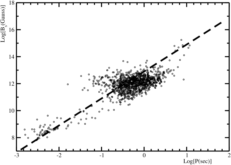
Figure 1: Inferred magnetic field $B_{S}$ plotted versus stellar period for 1194 pulsars taken from the ATNF Pulsar Catalog ATNF . Dashed line corresponds to Eq. (1) with $B_{1}\,\simeq\,1.3\,10^{13}\;Gauss$.

A straightforward consequence of Eq. (1) is that the dipolar magnetic field is time dependent. In fact, it is easy to find:

$$B_{S}(t)\;\simeq\;B_{0}\;\;\left(1\;+\;2\;\frac{\dot{P}}{P}\;t\;\right)\;\;\;\;,$$ (3)

where $B_{0}$ indicates the magnetic field at the initial observation time. Note that Eq. (3) implies that the magnetic field varies on a time scale given by the characteristic age:

$$\tau_{c}\;=\;\frac{P}{2\,\dot{P}}\;\;.$$ (4)

A remarkable consequence of Eq. (3) is that the effective braking index $n$ is time dependent. In particular, the braking index decreases with time such that:

$$-1\;\lesssim\;n\;\lesssim\;3\;\;,$$ (5)

the time scale variation being of order of $\tau_{c}/2$. However, it turns out that cea:2004b the monotonic derive of the braking index is contrasted by the glitch activity. Indeed, in our theory the glitches originate from dissipative effects in the inner core of the star leading to a decrease of the strength of the dipolar magnetic field, but to an increase of the magnetic torque. Moreover, we find that the time variation of the dipolar magnetic field could account for pulsar timing noise.

In the present paper we would like to discuss a fair general mechanism which allows to explain naturally pulsar radio emission as well as high energy emission. Our analysis is based on the remarkable dependence of the dipolar magnetic field on the spin period, Eq. (1), which seems to be supported by observational data. Even though such a dependence is natural within our P-star theory, one could follow a more pragmatic approach and merely assume the validity of Eq. (1) as a reasonable description of pulsar data.
In polar coordinate, the pulsar dipolar magnetic field $\vec{B}(\vec{r})$ for $r>R$, $R$ being the radius of the star, is given by:

$$\begin{split}B_{r}&=\;-\frac{2\;m\;\cos\theta}{r^{3}}\;\;,\\ B_{\theta}&=\;-\frac{m\;\sin\theta}{r^{3}}\;\;,\\ B_{\varphi}&=\;0\;,\end{split}$$ (6)

where:

$$m\;=\;B_{S}(t)\;R^{3}\;$$ (7)

is the magnetic moment. Note that, according to previous discussion we are assuming that the surface magnetic field strength is time dependent. Thus, from Maxwell equations

$$\vec{\nabla}\;\times\;\vec{E}\;=\;-\;\frac{\partial\;\vec{B}}{\partial\;t}\;,$$ (8)

where natural units $c=1$ are used, it follows:

$$E_{\varphi}=+\frac{\dot{m}\;\sin\theta}{r^{2}}\;\;\;,\;\;\;r\;>\;R\;\;\;.$$ (9)

Note that, according to Eq. (3) we have:

$$\dot{m}\;\simeq\;\;2\;B_{0}\;R^{3}\;\frac{\dot{P}}{P}\;\;\;,$$ (10)

so that:

$$E_{\varphi}\;\simeq\;\;2\;B_{0}\;\sin\theta\;\;\frac{\dot{P}}{P}\;\;\frac{R^{3}}{r^{2}}\;\;\;,\;\;\;r\;>\;R\;\;\;.$$ (11)

It is worthwhile to note that the induced azimuthal electric field Eq. (11) depends on the stellar period and period derivative. As we discuss below, it is this electric field which accounts for both radio and high energy emission.
In the following we work in the co-rotating frame of the star. We also assume that the magnetosphere contains a plasma whose charge number density is approximately the Goldreich-Julian charge density michel:1991 ; meszaros:1992 . These charges are accelerated by the induced azimuthal electric field $E_{\varphi}$ and thereby acquire an azimuthal velocity $v_{\varphi}$ which is directed along the electric field for positive charges and in the other direction for negative charges. Note that we do not need to separate positive charges from the negative ones, in other words we do not feel the current closure problem michel:1991 . Charged particles moving in the magnetic field $\vec{B}(\vec{r})$, Eq. (6), must emit electromagnetic waves, namely cyclotron radiation for non relativistic charges or synchrotron radiation for relativistic charges wallace:1977 . Obviously, radiation from electrons is far more important than from protons. So that in the following we shall consider electrons. For convenience, we also assume that electrons have positive charge $+e$. It turns out that electron cyclotron emission accounts for radio emission, while the synchrotron radiation is responsible for the high energy emission.
However, before addressing the problem of the emission spectra, it is worthwhile to discuss the distribution of the plasma in the region surrounding the pulsar (the magnetosphere). As we said before, charges are accelerated by the electric field $E_{\varphi}$, so that they are subject to the drift Lorentz force $\vec{F}\,=\,\vec{v}_{\varphi}\,\times\,\vec{B}(\vec{r})$, whose radial component is:

$$F_{r}=-v_{\varphi}B_{\theta}=+v_{\varphi}\;\frac{m\;\sin\theta}{r^{3}}\simeq+\;v_{\varphi}B_{0}\sin\theta\left(\frac{R}{r}\right)^{3},$$ (12)

while the $\theta$ component is:

$$F_{\theta}=+v_{\varphi}B_{r}=-v_{\varphi}\frac{m\cos\theta}{r^{3}}\simeq-v_{\varphi}B_{0}\cos\theta\left(\frac{R}{r}\right)^{3}.$$ (13)

The radial component $F_{r}$ pushes both positive and negative charges radially outward. Then, at large distances form the star the plasma must flow radially outward giving rise to the pulsar wind. On the other hand, $F_{\theta}$ leads to an asymmetric charge distribution in the upper hemisphere ($\cos\theta>0$) with respect to the lower hemisphere ($\cos\theta<0$). Indeed, $F_{\theta}$ is centripetal in the upper hemisphere and centrifugal in the lower hemisphere. As a consequence, in the lower hemisphere charges are pushed towards the magnetic equatorial plane $\cos\theta=0$. On the other hand, in the upper hemisphere the centripetal force gives rise to a rather narrow jet along the magnetic axis. Therefore, the emerging plasma distribution is a follows: a rather broad structure in the lower hemisphere, a narrow jet in the upper hemisphere, and an accumulation of plasma near the magnetic equatorial plane. Moreover, the drift force causes a continuous injection of charges from the lower hemisphere into the upper hemisphere. This, in turns, results in formation of plasma waves of large intensities propagating along the magnetic equatorial plane. It is remarkably that our qualitative discussion of plasma distribution around the pulsar turns out to compare rather well with recent observations of Crab and Vela pulsars pavlov:2001 ; helfand:2001 ; hester:2002 ; gaensler:2002 ; pavlov:2003 , after identifying the observed symmetry axis with the magnetic axis, and not with the rotation axis as usually assumed. Finally, it is worthwhile to point out that a fraction of the plasma injected into the upper hemisphere are eventually accelerated into the narrow jet. This process results into an acceleration of the pulsar giving a proper velocity directed along the magnetic axis and pointing in the direction opposite to the narrow jet.
Any further discussion of these points goes beyond the aim of the present paper. Here we shall focus on the emission processes capable of producing radiation at both radio and high energy frequencies. In particular, we do not attempt any precise comparison with available data, but we limit to estimate the relevant luminosities for typical pulsars.
In the following we assume as typical pulsar parameters:

$$\begin{split}P&\;\simeq\;1\;sec\;\;,\;\;\dot{P}\;\simeq\;10^{-14}\;,\;B_{0}\;\simeq\;10^{12}\;Gauss\\ R&\;\simeq\;10^{6}\;cm\;\;,\;\;I\;\simeq\;10^{45}\;gr\;cm^{2}\;.\end{split}$$ (14)

From Eq. (11) it follows that electrons acquire non relativistic azimuthal velocities farther out of the star, while they are relativistic near the star. So that non relativistic electrons moving in the magnetic field will emit cyclotron radiation, while relativistic electrons will emit synchrotron radiation. In both cases the radiated power is supplied by the azimuthal electric field $E_{\varphi}$. Let us, first, consider the cyclotron emission. As it is well known, most of the radiation is emitted almost at the frequency of rotation:

$$\nu(r)=\frac{eB(r)}{2\pi m_{e}}\simeq\frac{eB_{0}}{2\pi m_{e}}\left(\frac{R}{r}\right)^{3},$$ (15)

where $r$ is the radial distance from the star. From Eq. (15) it follows:

$$r\simeq R\left(\frac{eB_{0}}{2\pi m_{e}}\right)^{1/3}\frac{1}{\nu^{1/3}}\;.$$ (16)

To estimate the total power emitted we need to evaluate the power supplied by the azimuthal electric field. In the infinitesimal volume $dV=r^{2}\sin\theta drd\theta d\varphi$ the power supplied by the induced electric field $E_{\varphi}$ is:

$$d\dot{W}_{E_{\varphi}}\simeq 2n_{e}eB_{0}v_{\varphi}R^{3}\;\frac{\dot{P}}{P}\sin^{2}\theta drd\theta d\varphi\;,$$ (17)

where $n_{e}$ is the electron number density. Now, from Eq. (16) we get:

$$dr\simeq\frac{R}{3}\left(\frac{eB_{0}}{2\pi m_{e}}\right)^{1/3}\frac{1}{\nu^{4/3}}\;d\nu\;.$$ (18)

So that, integrating $d\dot{W}_{E_{\varphi}}$ over $\theta$ and $\varphi$, and using Eq. (18), we obtain the radiating spectral power:

$$F(\nu)\simeq\frac{2\pi^{2}}{3}n_{e}eB_{0}v_{\varphi}R^{4}\;\frac{\dot{P}}{P}\left(\frac{eB_{0}}{2\pi m_{e}}\right)^{1/3}\frac{1}{\nu^{4/3}}\;.$$ (19)

Few comments are in order. Firstly, in our model higher frequencies are generated near the star while lower frequencies further out. Indeed, our Eq. (16) gives a radius to frequency mapping which seems to be consistent with observations. The authors of Ref. kijak:1997 (for a recent review see Ref. graham-smith:2003 and references therein) argued that the emission altitude $r_{h}$ depends on pulsar period, period derivative and frequency according to:

$$r_{h}=\left(55\pm 5\right)R\;\tau_{6}^{-0.07\pm 0.3}\;P^{0.33\pm 0.5}\;\nu_{GHz}^{-0.21\pm 0.07}\;,$$ (20)

where $\tau_{6}$ is the characteristic age in units of $10^{6}$ years and $\nu_{GHz}$ is the frequency in units of $10^{9}\,Hz$. On the other hand, using Eqs. (2), (16) we get:

$$r\;\simeq\;\left(2.1\;10^{3}\right)R\;\;\dot{P}_{14}^{1/6}\;P^{1/6}\;\nu_{GHz}^{-1/3}\;,$$ (21)

where $\dot{P}_{14}$ is the period derivative in units of $10^{-14}$. The altitude $r_{h}$ is related to radial distance $r$ by:

$$r_{h}\;\simeq\;r\;\cos\theta\;\;.$$ (22)

We see that, if $\cos\theta\lesssim 0.1$ our Eq. (21) is in reasonable agreement with the semi-empirical relation Eq. (20). Note that $\cos\theta\lesssim 0.1$ means that the main origin of radiation is near the magnetic equatorial plane, in accord with our previous discussion on the plasma distribution. Second, our spectral power Eq. (21) displays a spectral index $\alpha\simeq-1.33$ in reasonable agreement with the observed typical spectral index. Moreover, the radial distance $r$ cannot exceed the light cylinder radius $R_{L}$. So that in general we have that $r\leq r_{break}$. It is natural to identify $\nu_{break}$, the frequency corresponding to $r_{break}$ according to Eq. (21), with the frequency where the observed radio spectrum displays a break. Usually it is found that $\nu_{break}\simeq 1~{}GHz$ graham-smith:2003 . Using the typical pulsar parameters, Eq. (14), we find $r_{break}\simeq R_{L}/3$, quite a reasonable result. To estimate the radio luminosity:

$$L_{Radio}=\int_{\nu_{break}}F(\nu)\;d\nu\;\;,$$ (23)

where the integration extends up to a frequency $\nu\gg\nu_{break}$, we assume as typical electron number density $n_{e}\simeq 10^{11}cm^{-3}$, and $v_{\varphi}\simeq 0.5$. In this way we obtain:

$$L_{Radio}\;\simeq\;1.3\;10^{27}\;erg/s\;\int_{1}\;\nu_{GHz}^{-4/3}\;d\nu_{GHz}\;,$$ (24)

or

$$L_{Radio}\;\simeq\;3.9\;10^{27}\;erg/s\;\;.$$ (25)

The spin-down power is given by:

$$-\;\dot{E}_{R}\;=\;4\;\pi^{2}\;I\;\frac{\dot{P}}{P^{3}}\;\simeq\;3.95\;10^{32}\;erg/s\;,$$ (26)

so that we get:

$$\frac{L_{Radio}}{|\dot{E}_{R}|}\;\simeq\;\;10^{-5}\;,$$ (27)

which is, indeed, the correct order of magnitude for typical observed radio luminosities manchester:1977 ; michel:1991 .
Essentially the same mechanism accounts for the high energy emission. Indeed, according to our previous discussion, in the region closer to the surface we expect that electrons will undergo ultra relativistic motion with Lorentz factor $\gamma\gg 1$. In this case the emitted radiation can be though of as a coherent composition of contributions coming from the components of acceleration parallel and perpendicular to the velocity. It turns out, however, that the radiation is mainly due to the perpendicular component. In the case of motion in a magnetic field the radiation spectrum will be mainly at the frequency schwinger:1949 (see also Ref. wallace:1977 ):

$$\omega_{m}\;\simeq\;\gamma^{2}\;\frac{eB}{m_{e}}\;.$$ (28)

So that, according to Eq. (6) we have:

$$\omega_{m}(r)\;\simeq\;\gamma^{2}\;\frac{eB_{0}}{m_{e}}\;\left(\frac{R}{r}\right)^{3}\;,$$ (29)

or

$$r\;\simeq\;R\;\gamma^{2/3}\;\left(\frac{eB_{0}}{m_{e}}\right)^{1/3}\frac{1}{\omega_{m}^{1/3}}\;.$$ (30)

Proceeding as before and using:

$$dr\;\simeq\;\frac{R}{3}\;\gamma^{2/3}\;\left(\frac{eB_{0}}{m_{e}}\right)^{1/3}\frac{1}{\omega_{m}^{4/3}}\;d\omega_{m}\;,$$ (31)

we get the high energy spectral power:

$$F_{HE}(\omega)\simeq\frac{2\pi^{2}}{3}\;n_{e}\;eB_{0}\;\gamma^{2/3}\;R^{4}\;\frac{\dot{P}}{P}\left(\frac{eB_{0}}{m_{e}}\right)^{1/3}\frac{1}{\omega^{4/3}}\;.$$ (32)

The high energy luminosity is:

$$L_{HE}\;=\;\int_{\omega_{HE}}F_{HE}(\omega)\;d\omega\;\;,$$ (33)

where again the integration extends up to $\omega\gg\omega_{HE}$, and $\omega_{HE}$ is the high energy break frequency emitted at radial distance $r_{HE}$. It is reasonable to assume that $r_{HE}\simeq 0.1\,r_{break}$. We further assume $\omega_{HE}\simeq 1MeV$, which leads to the estimate $\gamma\simeq 10^{5}$. Finally, using $n_{e}\simeq 10^{13}cm^{-3}$, we find for the high energy luminosity:

$$L_{HE}\;\simeq\;4.7\;10^{29}\;erg/s\;\;,$$ (34)

which in turns leads to:

$$\frac{L_{HE}}{|\dot{E}_{R}|}\;\simeq\;10^{-3}\;.$$ (35)

We see that also our high energy luminosity Eq. (35) compares rather well with observations.

In summary, we have discussed a fair general and simple mechanism for radio and high energy emission. Our results are based on the induced azimuthal electric field which accounts for plasma distribution in the region surrounding the pulsar, as well as for the radio and high energy luminosities. We have also discuss the formation of jet collinear with the magnetic axis, the pulsar wind and the possible origin of the pulsar proper motion velocities.

References

- (1) A. Hewish, S. G. Bell, J. D. H. Pilkington, P. F. Scott, and R. A. Collins, Nature 217, 709 (1968).
- (2) W. Baade and F. Zwicky, Proc. Nat. Acad. Sci. 20, 254 (1934); Phys. Rev. 45, 138 (1934); Phys. Rev. 46, 76 (1934).
- (3) R. N. Manchester and J. H. Taylor, Pulsars, (W. H. Freeman and Company, San Francisco, 1977).
- (4) F. Pacini, Nature 219, 145 (1968).
- (5) T. Gold, Nature 218, 731 (1968).
- (6) See, for instance, F. C. Michel, Rev. Mod. Phys. 54, 1 (1982); F. C. Michel, The State of Pulsar Theory , astro-ph/0308347.
- (7) F. C. Michel, Theory of Neutron Star Magnetospheres, (The University of Chicago Press, Chicago, 1991).
- (8) P. Mészáros, High-Energy Radiation from Magnetized Neutron Stars, (The University of Chicago Press, Chicago, 1992).
- (9) P. Goldreich and W. H. Julian, Astrophys. J. 157, 869 (1969).
- (10) P. A. Sturrock, Astrophys. J. 164, 529 (1971).
- (11) P. Cea, P-Stars, astro-ph/0301578.
- (12) P. Cea, RXJ1856.5-3754 and RXJ0720.4-3125 are P-Stars , astro-ph/0401339, to appear in JCAP.
- (13) P. Cea, Magnetic Fields and Glitches in P-Stars, in preparation.
- (14) http://www.atnf.csiro.au/research/pulsar/psrcat.
- (15) See, for instance: W. H. Wallace, Radiation Processes in Astrophysics (MIT Press, Cambridge, 1977); V. L. Ginzburg, Theoretical Physics and Astrophysics (Pergamon, Oxford, 1979).
- (16) G. G. Pavlov, O. Y. Kargaltsev, D. Sanwal, and G. P. Garmire, Astrophys. J. 544, L189 (2001).
- (17) D. J. Helfand, E. V. Gotthelf, and J. P. Halpern, Astrophys. J. 556, 380 (2001).
- (18) J. J. Hester, K. Mori, D. Burrows, J. S. Gallagher, J. R. Graham, M. Halverson, A. Kader, F. C. Michel, and P. Scowen, Astrophys. J. 577, L49 (2002).
- (19) B. M. Gaensler, J. Arons, V. M. Kaspi, M. J. Pivovaroff, N. Kawai, and K. Tamura, Astrophys. J. 569, 878 (2002).
- (20) G. G. Pavlov, M. A. Teter, O. Kargaltsev, and D. Sanwal, Astrophys. J. 591, 1157 (2003).
- (21) J. Kijak and J. Gil, MNRAS 288, 631 (1997).
- (22) F. Graham-Smith, Rep. Prog. Phys. 66, 173 (2003).
- (23) J. Schwinger Phys. Rev. 75, 1912 (1949).