Qualitative aspects of quasar microlensing with two mass components: magnification patterns and probability distributions

Abstract

It has been conjectured that the distribution of magnifications of a point source microlensed by a randomly distributed population of intervening point masses is independent of its mass spectrum. We present gedanken experiments that cast doubt on this conjecture and numerical simulations that show it to be false.

1 INTRODUCTION

Every investigation of microlensing at high optical depth that has explored the effect of multiple microlens mass components has led to the conclusion that the magnification probability distribution is independent of the spectrum of microlens masses. The recent effort by Wyithe & Turner (2001) is typical. While it was not their principal result, they comment in passing

“… we confirm the finding of Wambsganss (1992) and Lewis & Irwin (1995) that the magnification distribution is independent of the mass function.”

This conjecture has important consequences regarding the more general applicability of microlensing studies that are limited to a single mass component. While galaxies have stars with a range of masses, restricting to a single component makes analytic calculations more tractable (e.g. Peacock, 1986; Schneider, 1987; Kofman, Kaiser, Lee, & Babul, 1997) and greatly decreases the number of cases that must be simulated numerically (e.g. Wambsganss, 1992; Lewis & Irwin, 1995; Wyithe & Turner, 2001). If true, the conjecture simplifies things considerably.

Both theoretical and experimental lines of evidence lead to this conclusion, which has struck many investigators as obvious. On the experimental side, simulations like those carried out by Wyithe & Turner (2001) and their predecessors produce magnification histograms for different mass distributions that appear to be indistinguishable for fixed surface mass density and shear.

On the theoretical side, the high magnification tail of the magnification probability distribution has been shown to be independent of the microlens mass spectrum (Schneider, 1987). Moreover, Wambsganss, Witt, & Schneider (1992) showed that the average number of positive parity microimages depends only upon the surface mass density (or equivalently the convergence) and the shear. Since the scale free nature of gravity requires that the magnification probability distribution for a point source be the same for microlensing by a single mass of any size, it would appear strange if a mixture of two masses (at constant convergence and shear) produced a different magnification probability distribution.

There is, however, at least one argument against this apparently obvious conclusion, which we detail in $\S$ 2 below. It suggests that the magnification probability distribution does depend upon the mass spectrum. The argument suggests that the dependence would show up in a highly magnified negative parity macroimage – typically one of a close pair of images in a quadruply imaged quasar like PG1115+080.

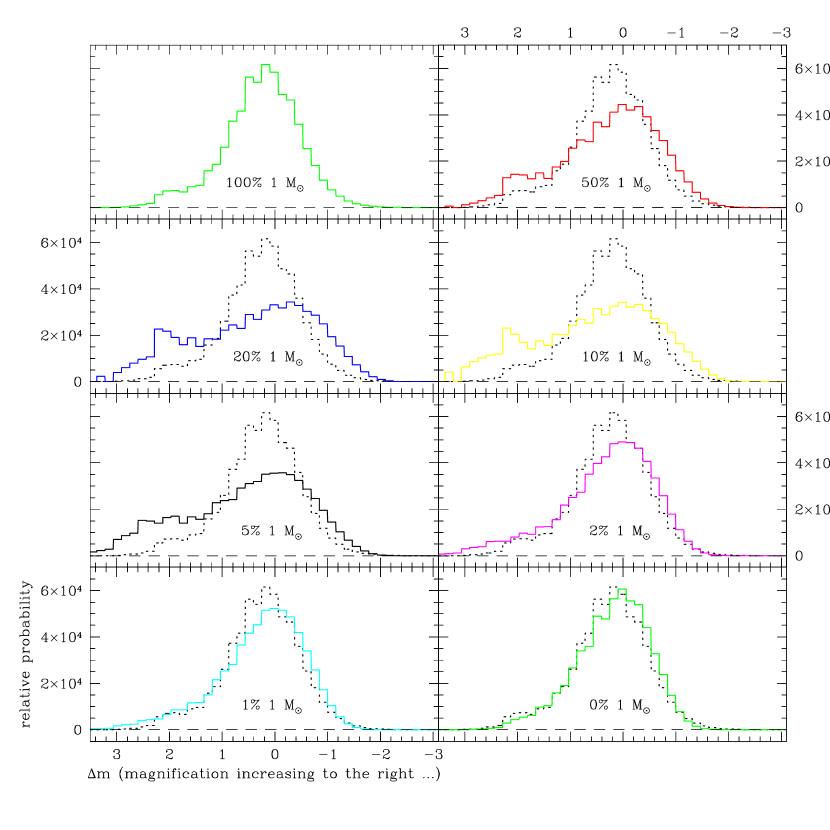
Figure 1: Magnification probability distributions for $\kappa_{tot}=\gamma=0.55$. The percentage in each panel denoted the fraction of $\kappa_{tot}$ composed of 1${\rm M_{\odot}}$ objects, the remainder being in 0.005${\rm M_{\odot}}$ masses. The dotted-line in each panel is the magnification probability distribution for the case where the entire microlensing population is comprised of 1${\rm M_{\odot}}$ object (presented in the upper left-hand panel).

We have carried out lensing simulations of such an image (at constant convergence and shear) for a variety of different cases. In Figure 1 we show simulations with two populations of point masses. The first component is comprised of $1.000{\rm M_{\odot}}$ objects referred to hereafter as “micro-lenses.” The second component is comprised of $0.005{\rm M_{\odot}}$ objects referred to hereafter as “nano-lenses.” The designations and mass scale are arbitrary but are intended to convey the sense that the micro-lenses are very much smaller than the lensing galaxy and that the nano-lenses are very much smaller than the micro-lenses.

The eight panels of Figure 1 show magnification histograms obtained by varying the mass fractions in the micro-lensing component, with the remaining fraction in the nano-lensing component. For the sake of comparison, we reproduce in each panel the result for a pure micro-lensing component. As the fraction contributed by micro-lenses decreases to 20% and 10% the histogram broadens out and develops a second peak. But as it decreases further to 0%, the magnification distribution narrows and ends up looking like the 100% case (modulo finite source effects and sample variance). Unless our simulations are faulty, the conjecture is false.

In $\S$ 2 we put forward a qualitative argument for the dependence of the microlensing probability distribution on the mass spectrum. In $\S$ 3 we give details of the numerical simulations that confirm the effect. In $\S$ 4 we offer a qualitative interpretation of our results. In $\S$ 5 we discuss some astrophysical consequences.

2 AN ARGUMENT FOR THE DEPENDENCE OF THE MAGNIFICATION PROBABILITY DISTRIBUTION ON THE MASS SPECTRUM

In Figure 2a we show the magnification probability distribution for a simulation of a negative parity macroimage with convergence $\kappa=0.55$ and shear $\gamma=0.55$. In this simulation all of the mass is in micro-lenses of a single mass. In Figure 2b we again show the magnification probability distribution for a simulation of a negative parity macroimage with convergence $\kappa=0.55$ and shear $\gamma=0.55$, but in this case 20% of the mass is in micro-lenses of a single mass and 80% of the mass is in a smooth mass sheet. The two histograms look quite different, with the first showing a single peak and the second being significantly broader and showing two peaks.

Now suppose that the smooth mass sheet of Figure 2b is divided into randomly distributed point masses that are very much smaller than the micro-lenses. We then have a micro-lensing component with $\kappa_{micro}=0.11$ and a nano-lensing component with $\kappa_{\rm nano}=0.44$. If the hypothesis that the magnification distribution is independent of the mass spectrum were correct, the magnification probability distribution would look the same as that of Figure 2a.

Finally, suppose we take our source to be extended rather than point-like. In particular, we imagine our source is much larger than the Einstein rings of our nano-lenses but much smaller than the Einstein rings of our micro-lenses. The nano-lenses should behave like a smooth component and the magnification probability distribution should look like Figure 2b.

Alternatively, we can compute the magnification probability distribution for our extended source by taking the magnification map for a point source and convolving it with the surface brightness distribution of the extended source. Such a convolution will inevitably smooth the map out, increasing the values of low magnification pixels and decreasing the values of high magnification pixels. If the conjecture were correct and the magnification histogram for a point source and macro- and nano-lensing components looked like Figure 2a, we would expect the magnification probability distribution for an extended source to be narrower.

Our two alternative schemes for computing the magnification histogram of an extended source lensed by a two component screen give different histograms, in one case broader and in the other case narrower than the histogram of Figure 2a. The histogram cannot simultaneously be both narrower and broader than that of Figure 2a. There is a bad link in one of the chains of argument, which we take to be the assumption that the magnification histogram for a point source is independent of the mass spectrum.

3 MICROLENSING SIMULATIONS

The particular values for the convergence, shear, and relative fractions in the two mass components used in the previous section were chosen (guided by the results of Granot et. al. 2003) to maximize the difference between Figures 2a and 2b. We have carried out microlensing simulations at the same convergence and shear, to look for differences in the microlensing histogram with different proportions of components.

The simulations were done employing the inverse ray-shooting method (Kayser, Refsdal, & Stabell, 1986; Schneider & Weiss, 1987) as described in Wambsganss (1990, 1999). We used a square receiving field of side length 20 Einstein radii $R_{E}$ (of the high mass component $m_{\rm micro}$). This area in the source plane was covered by 25 million pixels ($5000^{2}$). We used values of $\kappa_{\mathrm{t}ot}=0.55$ and $\gamma=0.55$ for surface mass density and external shear, corresponding to an (average) magnification of $|\mu|=10.0$ (negative parity). The positions of the lenses were distributed randomly in a circle significantly larger than the shooting region. The total number of rays per frame was typically about $n_{\mathrm{rays}}\approx 10^{10}$, resulting in over 200 rays per pixel on average (the shooting region was larger than the receiving region so that a significant number of rays landed outside the latter).

We performed a series of simulations with changing mass components. For the first series, we used two mass components with a mass ratio of $m_{\rm micro}/m_{\rm nano}=200$. For specificity we adopted $m_{\rm micro}=1{\rm M_{\odot}}$, appropriate to stars and $m_{\rm nano}=0.005{\rm M_{\odot}}$, as might apply to very massive planets.

We started with three cases: in the first case, 100% of the mass was in micro-lenses with mass $m_{\rm micro}$; in the second 50% of the micro-lenses were replaced with smooth matter; in the third case 50% of the matter was in nano-lenses with mass $m_{\rm nano}$ rather than in smooth matter.

The magnification maps for these simulations are displayed in Figure 3, with the left-hand panel presenting the full 20$R_{E}$, whereas the right-hand panel focuses upon a 1$R_{E}$ part of the map. For the smooth matter case (central panels) and the $m_{\rm nano}$ scenario (lowest panels), the location of the $m_{\rm micro}$ objects are the same.

In comparing the panels, it is apparent that the smooth matter and $m_{\rm nano}$ simulations possess similar large scale structure in their magnification maps, structure which is somewhat different from the case where all the mass is in $m_{\rm micro}$ objects. On smaller scales, however, the magnification patterns for the smooth mass and $m_{\rm nano}$ cases are quite different, with the presence of the smaller mass nano-lenses breaking up the magnification structure into smaller scale caustics.

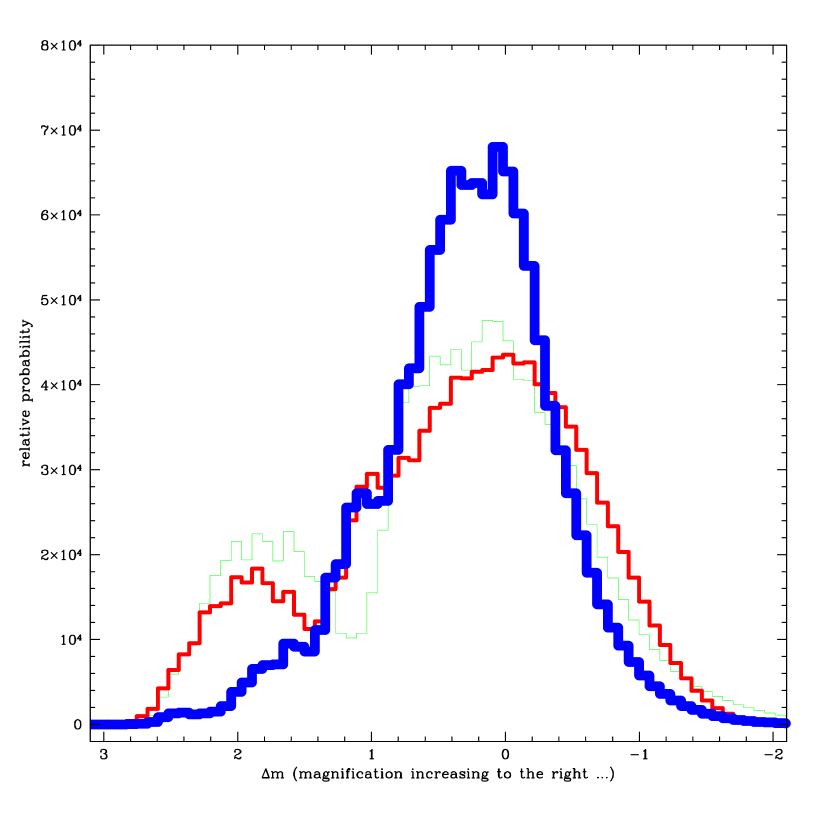
Figure 4: The magnification probability distributions for $\kappa_{tot}=\gamma=0.55$. The thick curve presents the case where all the mass is in 1${\rm M_{\odot}}$ objects, whereas the medium thickness curve is when 50% of $\kappa_{tot}$ is in 1${\rm M_{\odot}}$ objects and the remainder is in continuous matter. For the thin curve, this continuous matter contribution has been replaced by objects with a mass of 0.005${\rm M_{\odot}}$.

The magnification distributions for these simulations are presented in Figure 4. As discussed previously, the case where all the mass is in $m_{\rm micro}$ objects is unimodal, with the smooth matter case being bimodal . The case containing $m_{\rm nano}$ masses clearly differs from the solely $m_{\rm micro}$ case, also appearing bimodal and similar in form to the smooth matter case, at odds with the conjecture.

An examination of the magnification maps in Figure 3 illuminates the differences between the magnification distributions in Figure 4. Compared with the smooth matter map, the map for 100% $m_{\rm micro}$ has a higher density of caustics and fewer regions of demagnification (light-grey). These regions of the source plane produce no positive parity images. Crossing caustics produces extra positive parity images and additional magnification. These regions dominate the magnification histogram. In the smooth matter case, the magnification map has been ‘opened up,’ revealing more extended regions with no positive parity image and enhancing the low magnification peak seen in the magnification distribution. On large scales the magnification distribution for the 50% $m_{\rm nano}$ case resembles that of the smooth matter case, again with larger regions without positive parity images. Thus its magnification probability distribution looks more like that of the smooth matter case than that of the 100% $m_{\rm micro}$ case. Indeed the 50% $m_{\rm nano}$ case is even broader than the smooth case, due to the additional corrugation of the large scale map by the small scale lenses.

Further simulations were undertaken in an attempt to understand this difference. Again, we started with 100% micro-lenses, $m_{\rm micro}$. Then we put 1% of the total mass in nano-lenses, $m_{\rm nano}$, (re-)distributing them randomly over the lens plane. We increased the nano-lens mass fraction to 2%, 5%, 10%, and then proceeded in steps of 10% to 90%. We ended symmetrically with 95%, 98%, 99% and 100% nano-lenses, for a total 17 different cases. The numbers of lenses ranged from 25,000 (for 100% m_micro) to 2,600,000 (for 100% m_nano).

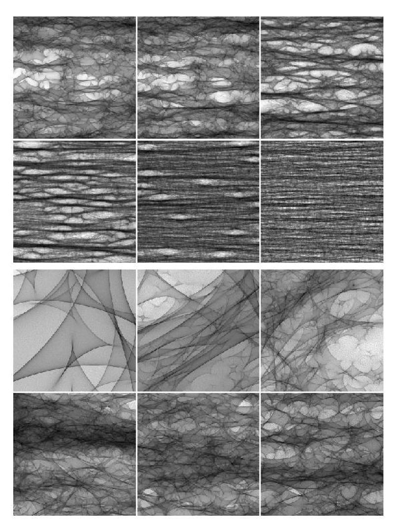
Figure 5: Magnification maps for the case $\kappa_{tot}=\gamma=0.55$. In the top six panels, the proportion of microlenses with a particular mass is changed such that (from left-to-right and top-to-bottom) the percentage of $\kappa_{tot}$ in 0.005${\rm M_{\odot}}$ objects is 0%, 20%, 60%, 90%, 98% & 100%; the remainder of $\kappa_{tot}$ is in 1${\rm M_{\odot}}$ masses in each case. Each magnification panel is $L=20R_{E}$ in extent. The size panels at the bottom show zooms of the lower left corners of the same sequence, respectively, sidelengths here are L = 1 $R_{E}$ (defined for a 1${\rm M_{\odot}}$-lens).

A selection of the resulting two dimensional magnification patterns is shown in Figure 5. The top six panels show the full simulation, while the bottom six panels show an expanded inset. Particularly notable is the similarity between the upper left panel (with all the mass in micro-lenses) and the lower right panel (the blowup of the map when all the mass is in nano-lenses). Simulations of this series were used to produce the histograms in Figure 1.

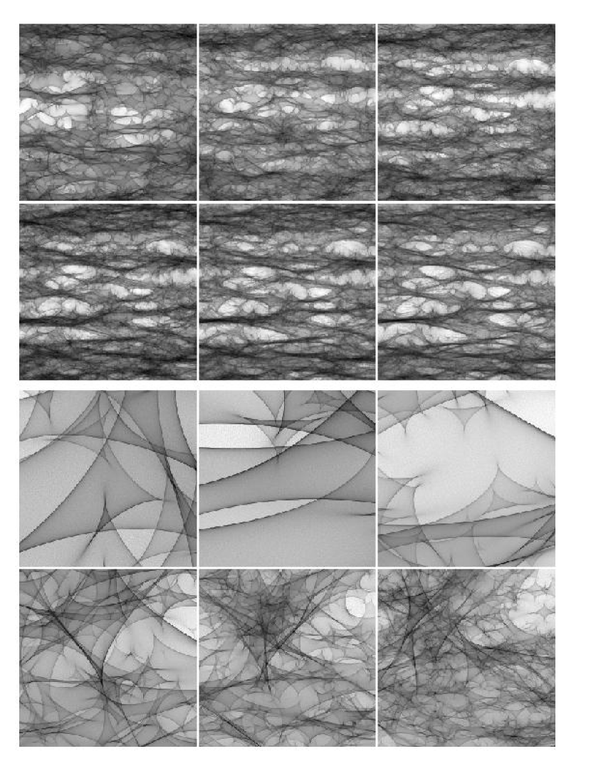
Figure 6: The top six panels present the magnification maps for the case $\kappa_{tot}=\gamma=0.55$. In each, 50% of $\kappa_{tot}$ is comprised of 1${\rm M_{\odot}}$ objects, while the remainder is composed of (top row, from left to right) 1${\rm M_{\odot}}$, $\sqrt{0.1}{\rm M_{\odot}}$, $0.1{\rm M_{\odot}}$, (second row) $\sqrt{0.01}{\rm M_{\odot}}$, $0.01{\rm M_{\odot}}$ and $\sqrt{0.001}{\rm M_{\odot}}$. Each panel is 20 $R_{E}$ in extent. The lower six panels present a zoom of the lower left-hand corner of the same magnification maps (extend is L = 1 $R_{E}$).

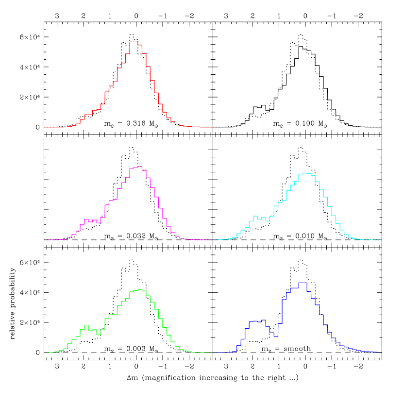
Figure 7: The six panels present the magnification distributions for a scenario with $\kappa_{tot}=\gamma=0.55$, and the matter being split between evenly two mass components (50% $m_{\rm micro}$, 50% $m_{\rm nano}$). The mass ratios are $m_{\rm micro}/m_{\rm nano}=0.316,0.100,0.032,0.01,0.003$ for the first five panels, and $m_{\rm nano}$ is assumed entirely smoothly distributed in the last panel. The dotted histogram is the respective panel for the case with 100% of the matter in $m_{\rm micro}$.

For the final series, we took 50% of the mass to be in micro-lenses, and 50% in nano-lenses, but let the masses of the nano-lenses vary with $m_{\rm nano}/m_{\rm micro}=0.32,0.10,0.032,0.01,$ and $0.0032$. As a bracketting cases we considered $m_{\rm nano}/m_{\rm micro}=1$ and the 50% smooth case, corresponding to $m_{\rm nano}/m_{\rm micro}\rightarrow 0$, making seven cases altogether. The magnification patterns for all but the smooth case are displayed in Figure 6. The magnification distributions are seen in Figure 7.

This last series shows that the conjecture fails only gradually. The presence of the second component becomes significant (for our simulation) only when the nano-lens masses are one tenth those of the micro-lenses. By the time the nano-lenses are one hundredth those of the micro-lenses, the effect is as large as we can measure. In hindsight this onset would have been more appreciable had we put 80% of the mass into nano-lenses (as in the third panel of Figure 1), but the qualitative effects would have been the same.

Our lensing simulations have two limitations:

• With the limited size of $L=20R_{E}$, the magnification maps exhibit features that are correlated on scales uncomfortably close to the size of the simulation volume. An ensemble of simulations with the same parameters will exhibit differences due to sample variance. We checked this for a few cases and found this sample variance to be small compared to the observed differences needed to make our case. Moreover, in the series of simulations described above, we kept the positions of the stars fixed to the extent possible, so that we could study the differential changes from one case to the next, and to hence minimize the effects of sample variance.

• The finite pixel size corresponds to a minimum source size, i.e. our results are not quite applicable to a point source. However, a size of $20R_{E}/5000{\mathrm{pix}}=0.004R_{E}/{\mathrm{pix}}$, is small enough for the effects we want to study and explore. This finite size unavoidably cuts off the magnification distribution at very high magnifications $\mu$ and leads to deviations from the power law behavior, but the low and intermediate magnification region we are interested in (see next section) is not strongly affected by that.

Despite the inevitable limited dynamic range for such simulations, we have tried to choose parameters such that we can demonstrate the effect most convincingly.

4 INTERPRETATION

In the previous section we simulated cuts through the $\kappa_{\rm nano}/\kappa_{\rm micro},m_{\rm nano}/m_{\rm micro}$ plane at fixed $\kappa_{tot}$ and $\gamma$. Somewhat counter-intuitively, we find that at fixed mass ratio $m_{\rm nano}/m_{\rm micro}=1/200$ the magnification probability histogram is broader for comparable amounts of two very different masses than it is for a single component of either one mass or the other.

The scale invariance of gravity demands that, for a point source, the magnification histograms of single components of very different masses should be identical. But our experiments show that for two very different mass components the magnification map looks very much like that of the higher mass component immersed in a perfectly smooth component. Only on small scales are there differences. This can be seen in Figure 3.

Suppose one grants that the magnification probability distribution for two very disparate components looks like that for a single component and a smooth component. The arguments set forth in (Rauch, Mao, Wambsganss, & Paczyński, 1992), Schechter and Wambsganss (2002) and Granot et al. (2003) would come into play: the magnification histogram tends to be broadest when the effective magnification computed from the effective convergence and the effective shear is of order $|\mu|\approx 3-4$. Alternatively, the fluctuations are largest when the number of extra positive parity images is roughly unity. In such cases one tends to get two peaks.

But the magnification probability distribution for two disparate components is not exactly that of a single component and a smooth component. The low mass component produces additional structure in the magnification map, further broadening the magnification histogram, rounding off its peaks and filling in its valleys. There is evidence for this in Figures 2 and 3.

Once one substitutes the low mass component for a smooth component, the number of extra positive parity images increases from roughly unity to something significantly larger. While this tends to round of the two peaks, it does not narrow the magnification histogram. The arguments of Schechter & Wambsganss (2002) and Granot et al. (2003) that the magnification histogram is broadest when there is, on average, one extra positive parity image does not hold for two disparate mass components. The reason is that the extra positive parity images cluster around the images produced by the single mass component, breaking them into pieces but only slightly changing the combined contribution to the flux.

5 ASTROPHYSICAL CONSEQUENCES

In gravitational lensing, magnifications depend upon second derivatives (with respect to position) of the time delay function (e.g. Blandford & Narayan, 1986). Deflections depend upon first derivatives. And time delays depend upon the function itself. The second derivatives are dimensionless, with the consequence that the magnification of an image (unlike its deflection and time delay) contains no information about the mass of intervening lens.

Image position fluctuations due to microlensing manifestly do contain information about the mass scale of the intervening microlenses (Lewis & Ibata, 1998; Treyer & Wambsganss, 2004, and references therein). Moreover the timescale over which brightness fluctuations occur likewise contains information about the mass scale of the intervening microlenses (and on the distribution of microlens masses) if one knows the relative velocities of the microlenses and the source (Wyithe & Turner, 2001). But the amplitude of those brightness fluctuations is independent of mass scale.

In the present paper we consider the dependence of brightness fluctuations not on mass scale, the first moment of the microlens mass distribution function, but on higher order dimensionless moments of that mass distribution. We have demonstrated (through our simulations using two mass components) that the magnification probability does depend upon those higher moments. We have not, however, explored the full range of astrophysically interesting mass distributions.

We have chosen to explore in detail the specific case of two mass components with $\kappa_{tot}=\gamma=0.55$, appropritate to one of two images in a highly magnified pair, as in the case of PG1115+080 (Young et al., 1981) or SDSS0924+0219 (Inada et al., 2003). The argument of Section 2 led us to believe that the effects of using two mass components rather than a single mass component would be appreciable in this case. But what about other values of the convergence and shear? How much does the mass spectrum matter for images of a quasar which are not saddle-points, or not highly magnified?

A thorough treatment of this question would explore a substantial fraction of the $\kappa,\gamma$ plane, and would quantify with some statistic the differences between a single mass component and a range of masses. Such a treatment lies beyond the scope of the present paper.

The fact that most previous investigators have failed to detect the effects of a range of microlens masses would argue that to first order such effects can be ignored. Even in the present case, where the convergence and shear have been chosen to maximize the effects, they are not large. Most mass distributions tend to put most of the mass at one or the other end of the mass distribution. The present simulations would seem to indicate that only if appreciable mass fractions are in components that differ by more than a factor of ten in mass will the effects of a range of masses be substantial.

6 ACKNOWLEDGMENTS

We gratefully acknowledge helpful conversations with Arlie Petters. GFL and JW thank M.I.T.’s Center for Space Resarch for its hospitality during a collaboratory visit during which much of this work was undertaken. GFL acknowledges losing a bottle of whiskey to PLS for backing the wrong horse. PLS gratefully acknowledges the whiskey. The work was supported in part by US NSF grant AST-020601.

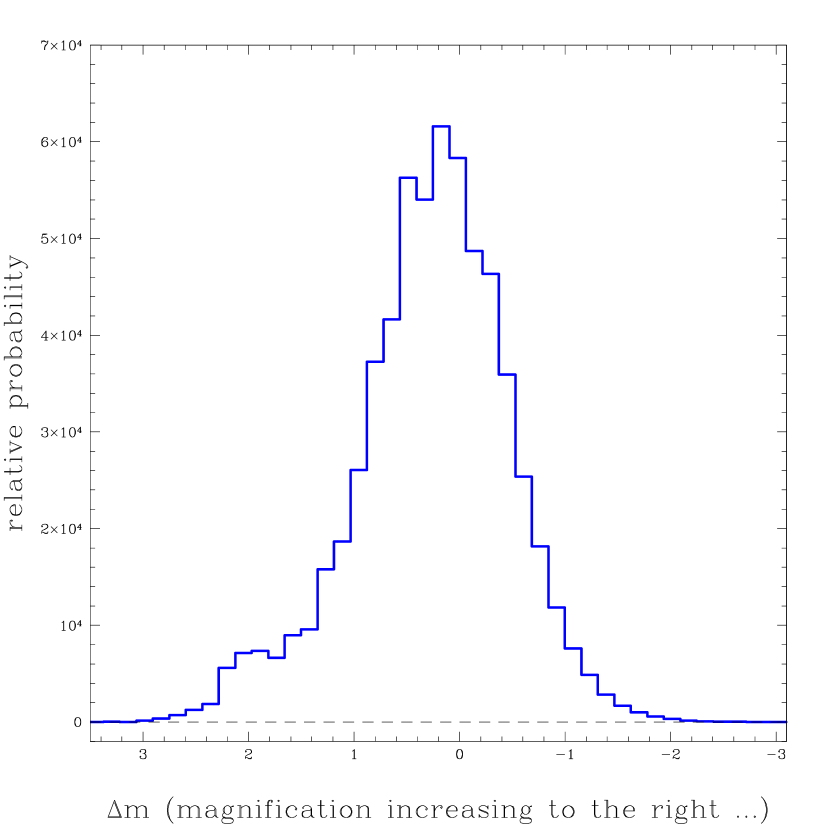
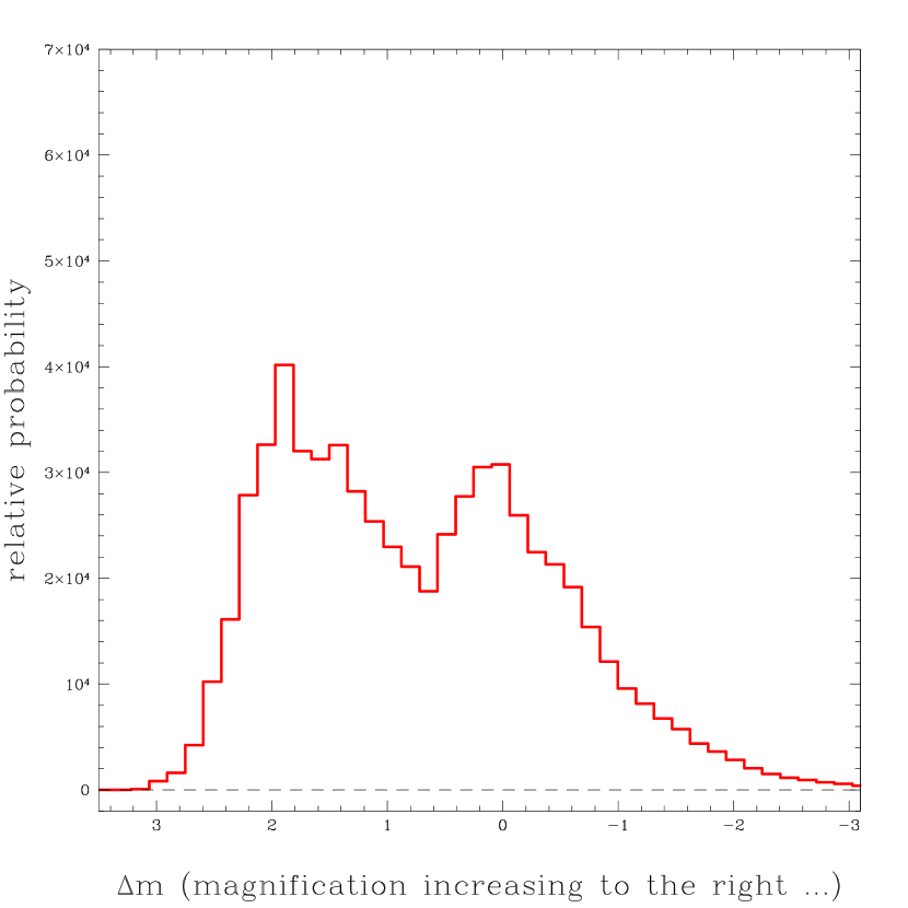
Figure 2: Magnification probability distributions for $\kappa_{tot}=\gamma=0.55$. On the left 100% of the matter is in $m_{\rm micro}=1{\rm M_{\odot}}$ objects. On the right 20% of the matter is in $m_{\rm micro}=1{\rm M_{\odot}}$ objects and 80% is in a smooth mass sheet.

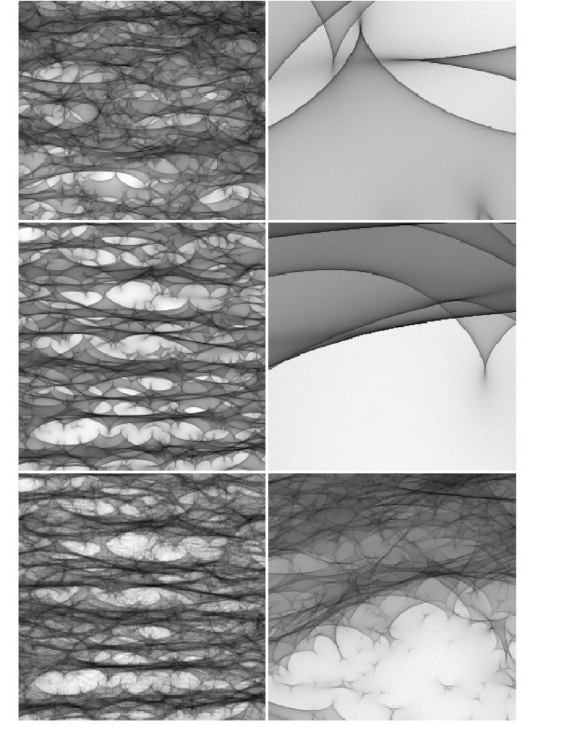
Figure 3: Magnification maps for the case with $\kappa_{tot}=\gamma=0.55$. The left-hand figures represent a region 20 $R_{E}$ (for a solar mass star) on a side. The right-hand panel is a zoom of the lower left-hand 1 $R_{E}$. The top row maps were constructed with $\kappa_{tot}$ all in 1${\rm M_{\odot}}$ masses, whereas the central panels consist of a microlensing population with 50% of $\kappa_{tot}$ in 1${\rm M_{\odot}}$ objects and the rest in continuous matter. The lower panels are for 50% of $\kappa_{tot}$ in 1${\rm M_{\odot}}$ objects and the remainder in 0.005${\rm M_{\odot}}$ masses.

References

- Blandford & Narayan (1986) Blandford, R. & Narayan, R. 1986, ApJ, 310, 568
- Granot, Schechter, & Wambsganss (2003) Granot, J., Schechter, P. L., & Wambsganss, J. 2003, ApJ, 583, 575
- Inada et al. (2003) Inada, N. et al. 2003, AJ, 126, 666
- Kayser, Refsdal, & Stabell (1986) Kayser, R., Refsdal, S., & Stabell, R. 1986, A&A, 166, 36
- Kofman, Kaiser, Lee, & Babul (1997) Kofman, L., Kaiser, N., Lee, M. H., & Babul, A. 1997, ApJ, 489, 508 s
- Lewis & Ibata (1998) Lewis, G. F. & Ibata, R. A. 1998, ApJ, 501, 478
- Lewis & Irwin (1995) Lewis, G. F. & Irwin, M. J. 1995, MNRAS, 276, 103
- Peacock (1986) Peacock, J. A. 1986, MNRAS, 223, 113
- Rauch, Mao, Wambsganss, & Paczyński (1992) Rauch, K. P., Mao, S., Wambsganss, J., & Paczyński, B. 1992, ApJ, 386, 30
- Schechter & Wambsganss (2002) Schechter, P. L. & Wambsganss, J. 2002, ApJ, 580, 685
- Schneider (1987) Schneider, P. 1987, ApJ, 319, 9
- Schneider & Weiss (1987) Schneider, P. & Weiss, A. 1987, A&A, 171, 49
- Seitz, Wambsganss, & Schneider (1994) Seitz, C., Wambsganss, J., & Schneider, P. 1994, A&A, 288, 19
- Treyer & Wambsganss (2004) Treyer, M. & Wambsganss, J. 2004, A&A, 416, 19
- Wambsganss (1990) Wambsganss, J. 1990, Ph.D. Thesis, University of Munich, Report MPA 550
- Wambsganss (1992) Wambsganss, J. 1992, ApJ, 386, 19
- Wambsganss (1999) Wambsganss, J. 1999, Journ. Comp. Appl. Math., 109, 353
- Wambsganss, Witt, & Schneider (1992) Wambsganss, J., Witt, H. J., & Schneider, P. 1992, A&A, 258, 591
- Wyithe & Turner (2001) Wyithe, J. S. B. & Turner, E. L. 2001, MNRAS, 320, 21
- Young et al. (1981) Young, P., Deverill, R. S., Gunn, J. E., Westphal, J. A., & Kristian, J. 1981, ApJ, 244, 723