Reduction of chemical networks

We analyse the evolution of the fractional ionisation in a steady-state protoplanetary disc over $10^{6}$ yr. We consider a disc model with a vertical temperature gradient and with gas-grain chemistry including surface reactions. The ionisation due to stellar X-rays, stellar and interstellar UV radiation, cosmic rays and radionuclide decay is taken into account. Using our reduction schemes as a tool for the analysis, we isolate small sets of chemical reactions that reproduce the evolution of the ionisation degree at representative disc locations with an accuracy of 50%–100%. On the basis of fractional ionisation, the disc can be divided into three distinct layers. In the dark dense midplane the ionisation degree is sustained by cosmic rays and radionuclides only and is very low, $\la 10^{-12}$. This region corresponds to the so-called “dead zone” in terms of the angular momentum transport driven by MHD turbulence. The ionisation degree can be accurately reproduced by chemical networks with about 10 species and a similar number of reactions. In the intermediate layer the chemistry of the fractional ionisation is driven mainly by the attenuated stellar X-rays and is far more complicated. For the first time, we argue that surface hydrogenation of long carbon chains can be of crucial importance for the evolution of the ionisation degree in protoplanetary discs. In the intermediate layer reduced networks contain more than a 100 species and hundreds of reactions. Finally, in the unshielded low-density surface layer of the disc the chemical life cycle of the ionisation degree comprises a restricted set of photoionisation-recombination processes. It is sufficient to keep about 20 species and reactions in reduced networks. Furthermore, column densities of key molecules are calculated and compared to the results of other recent studies and observational data. The relevance of our results to the MHD modelling of protoplanetary discs is discussed.

1 Introduction

Nowadays a paradigm of the evolution of a protoplanetary disc is widely accepted in which most of the disc matter is assumed to move steadily toward a protostar due to redistribution of the angular momentum. Ionisation in such objects is an important factor that enables the angular momentum transport to occur via magnetohydrodynamic (MHD) turbulence driven by the magnetorotational instability (MRI; Balbus & Hawley MRI (1991)). From this point of view, a disc is conventionally divided into the “active” layer, adjacent to the disc surface, and the “dead” zone, centred on the midplane. The active part of the disc is irradiated by high energy stellar/interstellar photons. Thus, the fractional ionisation there is relatively high, which implies that the magnetic field is well coupled to the gas. Due to this coupling, the active layer is unstable to the MRI, and the developing turbulence allows the accretion to occur (e.g., Gammie gammie (1996); Fleming & Stone fs2003 (2003)). The shielded midplane region is almost neutral, decoupled from the magnetic field, and, thus, quiescent.

The location of the boundary between these two regions may prove to be very sensitive to the disc physical properties and chemical composition (e.g., Fromang, Terquem, & Balbus from2002 (2002)). However, the MHD modelling with non-ideal effects included is a very demanding computational task. This is why in the MHD modelling of protoplanetary discs (and protostellar clouds) a very simple chemical scheme is usually assumed with a few ions and a network that includes only ionisation and recombination reactions, often neglecting the presence of dust grains (Sano et al. sano (2000); Fromang et al. from2002 (2002); Fleming & Stone fs2003 (2003)). The medium is believed to be in chemical equilibrium so that the fractional ionisation $x_{\mathrm{e}}$ can be expressed as (e.g., Gammie gammie (1996))

$$x_{\mathrm{e}}(\mathrm{eq})=\sqrt{\zeta\over\beta n_{\mathrm{H}}},$$ (1)

where $\zeta$ is the ionisation rate, $\beta$ is a typical recombination coefficient, and $n_{\mathrm{H}}$ is the hydrogen number density. This approach may indeed be valid if only the cosmic ray ionisation is taken into account and only gas-phase chemical processes are considered. However, dust plays an important role in the evolution of the fractional ionisation being an efficient electron donor for recombining ions and a sink for neutrals in cold parts of a disc. Moreover, newly born stars possess a relatively high X-ray flux with photon energies from about 1 to 5 keV (e.g. Igea & Glassgold IG99 (1999)). These factors give rise to a more complicated chemistry relevant for the ionisation degree. In particular, different ions dominate the fractional ionisation at different times and in different parts of the disc. Therefore, the straightforward application of Eq. (1) for evaluating the ionisation degree can be fraught with errors in some parts of a disc.

To check the validity of Eq. (1), we analyse the detailed ionisation structure of a protoplanetary disc computed with the full UMIST 95 chemical network (Millar et al. umist95 (1997)) with the surface chemistry included. We adopt a reference disc model to serve as a guide to the range of possible physical conditions that may be encountered in real protoplanetary objects. Within this model, we choose several representative disc locations and investigate in detail which chemical processes control the time-dependent ionisation degree there. Our intention is to show that the oversimplified treatment of the ionisation in a protoplanetary disc as an equilibrated ionisation-recombination cycle can lead to $x_{\mathrm{e}}$ values that differ by more than an order of magnitude from values computed with all the available information on the disc chemical evolution.

We describe the chemical processes that are responsible for ionisation in a disc in terms of reduced networks that are subsets of the full UMIST 95 network, supplied in some cases by a few surface reactions. These networks contain only those species and reactions that are needed to reproduce $x_{\rm e}$ with up to a factor of 2 uncertainty. The utilised reduction methods are described in Wiebe, Semenov & Henning (papi (2003), hereafter Paper I). The species-based reduction rests upon the Ruffle et al. (Rea02 (2002)) technique and consists of choosing species that are important in a particular context, and then selecting from the entire network only those species that are necessary to compute abundances of important species with a reasonable accuracy. In the reaction-based method, analysis starts from reactions that govern the abundance of important species. All reactions in the entire network are assigned weights according to the influence they have on abundances of important species. Then, only those reactions are selected that have weights above a cut-off parameter that is selected on the basis of the requested accuracy. Only those species are included in the reduced network that participate in selected reactions.

The organisation of the paper is the following. In Section 2 we describe the disc model and its physical structure as well as updates to the chemical model of Paper I. In Section 3 we discuss the initial conditions for the disc chemistry. The processes responsible for the fractional ionisation in various parts of the disc are outlined in Section 4. In Section 5 column densities are tabulated and compared to other studies and observational data. Results of the analysis and their relevance to the MHD modelling are discussed in Section 6. Final conclusions are drawn in Section 7.

2 Disc model and physics update

2.1 Disc structure and parameters

As a basis for our calculations, we adopted the steady-state disc model of D’Alessio et al. (DALdisc (1999)). The central star is assumed to be a classical T Tau star with an effective temperature $T_{*}=4\,000$ K, mass $M_{*}=0.5M_{\odot}$, and radius $R_{*}=2R_{\odot}$. The disc has a radius of 373 AU, an accretion rate $\dot{M}=10^{-7}\,M_{\odot}$ yr^-1, and viscosity parameter $\alpha=0.01$. It is illuminated by UV radiation from a central star and by interstellar UV radiation. The intensity of the stellar UV field is described with the standard $G$ factor, which is scaled in a way that the unattenuated stellar UV field at $R=100$ AU is a factor of $10^{4}$ stronger than the mean interstellar radiation field (Draine Draine (1978)). The visual extinction of stellar light at a given disc point is calculated as

$$A_{\mathrm{V}}={N_{\mathrm{H}}\over 1.59\cdot 10^{21}}\leavevmode\nobreak\ \frac{\mathrm{mag}}{\mathrm{cm}^{-2}},$$ (2)

where $N_{\mathrm{H}}$ is the column density of hydrogen nuclei between the point and the star. The extinction of the interstellar UV radiation is computed in a similar way (but in a vertical direction only).

In addition to the UV field, three other ionisation sources are considered: cosmic ray ionisation ($\zeta_{\mathrm{CR}}$), decay of radionuclides ($\zeta_{\mathrm{R}}$), and stellar X-ray ionisation ($\zeta_{\mathrm{X}}$). The following expression is used to compute the cosmic ray ionisation rate:

$$\begin{array}[]{l}\zeta_{\mathrm{CR}}=\\ \quad\frac{1}{2}\zeta_{0}\left[\exp\left({-\Sigma_{1}(z,r)/10^{2}}\right)+\exp\left({-\Sigma_{2}(z,r)/10^{2}}\right)\right],\\ \end{array}$$ (3)

where $\Sigma_{1}(z,r)$ is the surface density (g cm^-2) above the point with height $z$ at radius $r$, $\Sigma_{2}(z,r)$ is the surface density below the point with height $z$ at radius $r$, and $\zeta_{0}=1.3\cdot 10^{-17}$ s^-1. Thus, we assume that cosmic ray particles penetrate the disc only in the vertical direction from both its surfaces. The X-ray ionisation rate $\zeta_{\mathrm{X}}$ is computed according to Glassgold, Najita & Igea (1997a ; 1997b ) with parameters for their high depletion case. The source of X-rays is assumed to be located at $z=12\,R_{\odot}$. We adopt the ionisation rate due to decay of radioisotopes to be $\zeta_{\mathrm{R}}=6.5\cdot 10^{-19}$ s^-1.

The region under investigation spans a range of radii from 1 to 373 AU. We do not consider regions closer to the star to avoid the necessity to account for physical processes like dust destruction and collisional ionisation. Even when the close vicinity of the star is excluded, the disc is still characterised by a wide range of all relevant physical parameters: gas temperatures $T_{\mathrm{g}}$ are $10-600$ K, densities are $10^{-20}-10^{-10}$ g cm^-3, $G$ are $10^{2}-10^{8}$, $A_{\mathrm{V}}$ varies from 0 to more than 100 mag and ionisation rates are $10^{-18}-10^{-10}$ s^-1.

We divide the disc into three regions, namely, the midplane, the intermediate layer, and the surface layer. This division is similar to that outlined by Aikawa & Herbst (ah1999 (1999)). The midplane is the part of the disc near the symmetry plane, which is opaque to both X-ray and UV photons and is ionised primarily by cosmic ray particles. If one goes up from the midplane, the fractional ionisation first stays the same as in the midplane, but then at some height it starts to grow in response to increasing X-ray intensity. We take this turn-off height to be the lower boundary of the intermediate layer (and the upper boundary of the midplane region). In our model this height is approximately given by $z_{\mathrm{L}}=0.05\,r^{1.42}$ AU. With increasing height, the fractional ionisation grows first slowly, then much faster, in response to the decreasing opacity of the medium. The point where transition between slow and fast growth occurs is assumed to be the upper boundary of the intermediate layer and the lower boundary for the third, surface layer. This boundary is approximated by $z_{\mathrm{U}}=0.17\,r^{1.27}$ AU. The fractional ionisation is important in dynamical calculations only if it is small, as high ionisation means that the ideal MHD equations can be used. Thus, we set the upper boundary of the surface layer to a position where the ionisation degree exceeds $\sim 10^{-4}$. This simple picture may not be appropriate if diffusion processes or radial transport of the disc matter are taken into account (Ilgner et al. IHMM03 (2003)).

The disc structure is depicted in Figure 1. The upper boundary of the surface layer is shown schematically (thick solid line), as at $R\ga 100$ AU it extends beyond the disc limits (dotted line) for the adopted cut-off fractional ionisation of $10^{-4}$. In Figure 2 we show the dependence of the fractional ionisation on the height above the disc plane computed with the chemical model, described below, for several representative radii $R$.

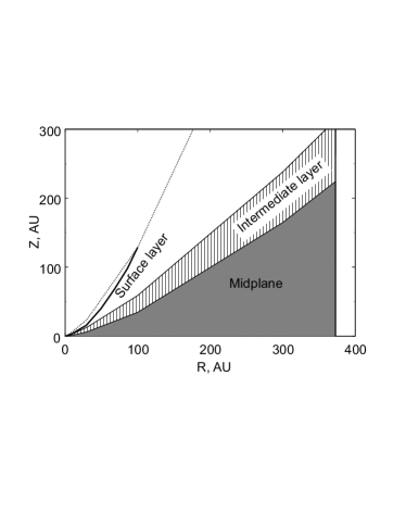
Figure 1: Three layers of a disc with distinctively different sets of chemical processes responsible for the value of the fractional ionisation $x_{\mathrm{e}}$. The thick solid line is the upper boundary of the surface layer where $x_{\mathrm{e}}=10^{-4}$, while dotted line depicts the disc upper limits.

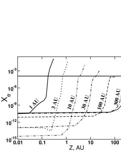
Figure 2: Fractional ionisation as a function of height above the disc plane. Lines are labelled with the corresponding radii.

2.2 Chemical model

The chemical model used in this paper is essentially the same as in Paper I, but with a few corrections that are described in this subsection. We adopt the UMIST 95 ratefile (Millar et al. umist95 (1997)) for the gas-phase chemistry and the surface reaction set compiled by Hasegawa, Herbst & Leung (hhl92 (1992)) and Hasegawa & Herbst (hh93 (1993)). As we have multiple ionisation sources in the protoplanetary disc, the cosmic ray ionisation rate is replaced by the sum $\zeta_{\mathrm{CR}}+\zeta_{\mathrm{X}}+\zeta_{\mathrm{R}}$ in expressions for rates of chemical reactions with cosmic ray particles (CRP) and cosmic ray induced photoprocesses. Given the high intensity of the impinging UV radiation, photodesorption of surface species is taken into account along with other desorption mechanisms.

2.2.1 Grain charge

The major difficulty in modelling the fractional ionisation in a dark and dense environment, like a protoplanetary disc midplane, is that grains play a very important role in ion recombination and can be the dominant charged particles in some disc regions. The charge of grains and, consequently, their impact on the local dynamics can sensitively depend on the grain size distribution, icy mantle composition etc. (e.g. Nishi, Nakano & Umebayashi Nishi (1991)). Thus, the computation of the fractional ionisation in the disc midplane is related not only to the chemistry but to the grain physics as well. This means we should include at least a simplified treatment of grain charging processes in the model.

The following changes are made with respect to Paper I. We consider neutral, positively charged, and negatively charged grains separately. A grain attains a negative charge or loses a positive charge colliding with free electrons. The probability of an electron sticking to grain surfaces is assumed to decrease exponentially with dust temperature $T_{\mathrm{d}}$, so that the sticking coefficient is around 0.5 at $T_{\mathrm{d}}\sim 10-20$ K, close to the value obtained by Umebayashi & Nakano (un1980 (1980)), and is essentially zero at higher temperatures. Via dissociative recombination of a gas-phase ion, a grain loses one electron and becomes neutral or positively charged. Rates of collisions between electrons and positively charged grains are multiplied by a factor, correcting for the long-distant Coulomb attraction, $C_{\rm ion}=1+e^{2}/ka_{\rm d}T_{\rm d}$, where $a_{\mathrm{d}}=0.1\leavevmode\nobreak\ \mu$m is the grain radius. It is always assumed that $T_{\rm g}=T_{\rm d}=T$.

2.2.2 Sticking probability

In Paper I the sticking probability $S$ was taken to be 0.3 at $T_{\rm g}=10$ K for all neutral species except H, He, and H₂. However, at higher temperatures $S$ is likely to be smaller (Burke & Hollenbach BH1983 (1983)). To account for this tendency, we multiply $S$ for neutrals by an additional factor equal to the fraction of molecules of a given kind that have thermal energy lower than the desorption energy $E_{\rm D}$ for this species (assuming a Maxwellian velocity distribution).

2.2.3 Desorption processes

The disc model, used in this paper, is characterised by a much wider range of physical conditions than the model for a molecular cloud considered in Paper I. This means, in particular, that changes must be made to the adopted model of the species desorption from grain surfaces. First, we now have the UV radiation in the model, so we add photodesorption to the processes listed in Paper I. The rate of photodesorption is given by

$$k_{\rm ph}=\left[G_{\mathrm{S}}\exp(-2A_{\mathrm{V}}^{\rm S})+G_{\mathrm{IS}}\exp(-2A_{\mathrm{V}}^{\rm IS})\right]Y\pi a_{\rm d}^{2},$$ (4)

where $G_{\mathrm{S}}$ and $G_{\mathrm{IS}}$ are intensities of the stellar and interstellar UV radiation expressed in units of the mean interstellar radiation field, $A_{\mathrm{V}}^{\rm S}$ and $A_{\mathrm{V}}^{\rm IS}$ are the corresponding visual extinctions in the direction to the star and in the vertical direction, and $Y$ is the photodesorption yield for which we adopted the expression

$$Y=0.0035+0.13\exp(-336/T_{\rm d}),$$ (5)

derived by Walmsley, Pineau des Forêts & Flower (wpf1999 (1999)) from the experimental data obtained by Westley et al. (westley (1995)).

The cosmic ray desorption rate also needs to be revised. The expression suggested by Hasegawa & Herbst (hh93 (1993)) and used in Paper I is based on the assumption that a cosmic ray particle (usually an iron nucleus) deposits on average 0.4 MeV into a dust grain of the adopted radius, impulsively heating it to a peak temperature $T_{\rm crp}$, which is close to 70 K for cold $0.1\mu$m silicate dust. As in a disc we expect much higher dust temperatures, data from Léger, Jura & Omont (leger (1985)) are used to take into account the dependence of the cosmic ray heating on the initial dust temperature. The peak temperature is approximated as

$$T_{\rm crp}=(4.36\cdot 10^{5}+T_{\rm d}^{3})^{1/3}.$$ (6)

This expression predicts that a grain heats up to 76 K at $T_{\rm d}=10$ K and gives almost no heating for $T_{\rm d}\ga 100$ K.

3 Initial conditions for chemistry

The problem of the initial conditions for chemical models of star-forming regions remains an open issue. The modelling of pre-protostellar objects commonly starts with the purely atomic or partly ionised initial composition, while in reality the initial abundances even for a moderately dense medium must reflect its previous evolution which ideally would have started from a diffuse intercloud gas. Even though the atomic or ionic initial composition can be adequate in the prestellar or pre-protostellar objects, the situation is different in protoplanetary discs, where the chemical composition at the beginning of the modelling is obviously far more advanced. One way to cope with this problem is to use “sliding” initial conditions, when the initial abundances are set to be mostly atomic at the outer radius of the disc. Then, a chemical model is run, and the final abundances at a given radius are used as initial abundances at the next radius, closer to the disc centre (Bauer et al. bauer (1997); Willacy et al. willacy (1998)). Another approach is to compute the input abundances with the model of a dark cloud, out of which the disc has evolved (e.g. Aikawa & Herbst ah1999 (1999); Aikawa et al. warm (2002)). Willacy et al. (willacy (1998)) compared both methods and found that, with a few exceptions, they provide similar results, because in a high-density environment reasonable molecular abundances are reached within a fraction of a year even with the atomic initial composition.

To simplify the reduction, we adopted the second approach. The choice of a cloud model in Aikawa et al. (warm (2002)) and in previous papers of this group is based on the analysis of the Ohio New Standard Model performed by Terzieva & Herbst (1998a , 1998b ). These authors developed a simple composite criterion that allows one to estimate how good the chemical model is in reproducing the chemical composition of a given object. Adopting a fixed density of $2\cdot 10^{4}$ cm^-3 and a gas temperature of 10 K, Terzieva & Herbst (1998a ) found that with the pure gas-phase chemistry, the chemical composition of the two typical molecular clouds, namely, TMC-1 and L134N, is best reproduced after about $3\cdot 10^{5}$ years of the evolution. Aiming to reproduce the observed low abundances of water and molecular oxygen, Roberts & Herbst (rh2002 (2002)) added surface chemistry to this model and found that the “best consistency” interval can be shifted toward a somewhat later time, like a few times $10^{6}$ years.

As we use the UMIST 95 ratefile, we perform a similar analysis for this database. The observed abundances for TMC-1 and L134N are taken from Ohishi, Irvine & Kaifu (ohishi (1992)) and Langer et al. (h2c6 (1997)). Following Terzieva & Herbst (1998b ), we assume that the abundance of a given molecule is consistent with observational data if it lies within an order of magnitude of the observed abundance. When the observed abundance is an upper limit, we assume that the computed abundance is in agreement with observations if it is less than or equal to 10 times this upper limit. With the same density, temperature and the surface chemistry included, we find that for our chemical model the agreement is best at $t\sim 10^{6}$ years (Fig. 3). The “low-metal” set of abundances from Paper I is adopted for this computation.

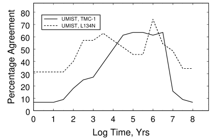
Figure 3: Percentage agreement between calculated and observed gas-phase abundances.

We now use the set of gas-phase and surface abundances, obtained with the above model for $t=10^{6}$ years as the initial conditions. The brief outline of this set is the following (abundances relative to the number of hydrogen nuclei are given in parentheses): The primary carbon-bearing compound is surface formaldehyde ($3.7\cdot 10^{-5}$) which also accounts for a significant fraction of the overall oxygen content, being second only to surface water ($7.8\cdot 10^{-5}$). Gas-phase oxygen and carbon are locked in CO molecules ($2.8\cdot 10^{-5}$). A fraction of oxygen is also present in atomic ($1.1\cdot 10^{-5}$) and molecular ($8.7\cdot 10^{-6}$) form. Gas-phase nitrogen is contained mainly in N₂ molecules ($9.7\cdot 10^{-6}$), while in icy mantles the main N-bearing species are HCN and HNC ($\sim 10^{-6}$ each) with a slightly lower amount of CH₂NH, NH₃, and NO. Sulphur is distributed almost equally between gas and dust phases. In the gas-phase it is locked in the CS molecules ($2.9\cdot 10^{-8}$). Surface sulphur is bound in H₂S ($2.2\cdot 10^{-8}$) and H₂CS ($1.5\cdot 10^{-8}$). Even though the density is not very high, metals are already significantly depleted. Surface abundances of Mg, Fe, and Na constitute about 1/3 of their total abundances. The dominant ions are HCO⁺ ($3.8\cdot 10^{-9}$), H${}_{3}^{+}$ ($3.5\cdot 10^{-9}$), Mg⁺ ($1.9\cdot 10^{-9}$), C⁺ ($1.3\cdot 10^{-9}$), and Fe⁺ ($1.2\cdot 10^{-9}$).

It should be kept in mind that some of our reduced networks computed for this initial composition may not be appropriate for purely atomic initial abundances of for abundance sets with higher metal content.

Table 1: Dominant ions in the midplane, intermediate layer and surface layer at $t=10^{6}$ years.

R, AU	1	3	10	30	100	300	373
Midplane	Na+	HCNH+	HCO+	HCO+	N2H+	H${}_{3}^{+}$	H${}_{3}^{+}$
Intermediate	Mg+	HCO+	HCO+	HCO+	HCO+	HCO+	HCO+
layer		S+
		H${}_{3}^{+}$
		and others
Surface	C+	C+	C+	C+	C+	C+	C+
layer	H+	H+

4 Chemistry of the ionisation degree in a protoplanetary disc

In each of the selected disc points the chemical model described in Section 2 is run up to $t=10^{6}$ years. Dominant ions in various disc domains are listed in Table 1. Reduction methods are then used to find those processes that determine $x_{\rm e}$. All the reduced networks described in this section are freely available from the authors. Also, we show some representative networks for the midplane and the surface layer.

4.1 Ionisation in the midplane

The midplane of the disc is characterised by high density, high optical depth and a relatively low ionisation rate. Neither the UV radiation from a central star nor the interstellar UV radiation is able to penetrate into this region. The ionisation rate is close to $10^{-17}$ s^-1. At the point closest to the star, $\zeta$ is dominated by X-ray ionisation; further away from the centre the attenuated cosmic rays are the only ionising factor. The temperature drops from $\sim 600$ K at $R=1$ AU to about 8 K at the disc edge. In the same distance interval, the gas density goes down from $10^{-10}$ g cm^-3 to less than $10^{-14}$ g cm^-3. Detailed physical conditions for the midplane are given in Table 2.

Table 2: Physical conditions in the midplane.

No.	$R$, AU	$\rho$, g cm-3	$T$, K	$\zeta_{\rm CR}$, s-1	$\zeta_{\rm X}$, s-1
M1	1.	2.1($-$10)	614.	8.8($-$19)	7.5($-$18)
M2	3.	4.7($-$11)	193.	2.3($-$18)	4.0($-$23)
M3	10.	8.5($-$12)	52.	5.0($-$18)	1.2($-$25)
M4	30.	7.3($-$13)	29.	9.4($-$18)	5.4($-$27)
M5	100.	4.8($-$14)	16.	1.2($-$17)	3.8($-$28)
M6	300.	4.8($-$15)	9.	1.3($-$17)	4.0($-$29)
M7	370.	3.3($-$15)	8.	1.3($-$17)	2.6($-$29)

4.1.1 Dark, hot chemistry

Table 3: Reduced network for dark, hot chemistry in the midplane.

${\rm NO}^{+}+{\rm Mg}$	$\rightarrow$	${\rm Mg}^{+}+{\rm NO}$
${\rm Mg}^{+}+e^{-}$	$\rightarrow$	${\rm Mg}+h\nu$
${\rm NO}+h\nu_{\rm CR}$	$\rightarrow$	${\rm NO}^{+}+e^{-}$

The chemistry of the point M1 (see Table 2) is extremely simple. In essence, it involves only five species, which are neutral and ionised magnesium, neutral and ionised NO, and electrons. The reduced network for this point is shown in Table 3. At the beginning of the computation the electron abundance decreases from the initial value of $\sim 10^{-9}$ to the new equilibrium value of about $10^{-11}$, determined by the electron exchange between Mg, Mg⁺, NO, and NO⁺, and then remains nearly constant. With the full network, the dominant ion is Na⁺, but it serves mainly as a passive sink for positive charges. This is why it is taken out of the reduced network. It suffices to include ionised magnesium, which is one of the most abundant ions in the initial abundance set.

Note the apparent similarity of this network to the one that determines $x_{\rm e}$ in dense interstellar clouds (Oppenheimer & Dalgarno OD74 (1974)) in the sense that it consists of a representative metal, a representative molecular ion and the charge transfer reaction between them. The explanation is that, even though we include gas-grain interaction in our model, at such high temperature the chemistry mostly proceeds in the gas-phase. Thus, the ionisation degree is determined by gas-phase reactions. However, due to much higher density these reactions are different from those described in Oppenheimer & Dalgarno (OD74 (1974)). The major difference is that the reaction of H₂ ionisation by cosmic rays is not important in the considered point. A modest electron supply is provided by NO ionisation by cosmic ray induced photons. The importance of the NO⁺ ion is determined by its chemical inertness. Due to this inertness, most of the time its abundance exceeds that of other ions, involved in charge transfer reactions with magnesium, by more than an order of magnitude. With this $5\times 3$ network, the error in the fractional ionisation does not exceed 40% during the entire computation time. By adding a few more species to the reduced network, it is possible to decrease this uncertainty to 20%. These species account for the rapid destruction of the two other initially abundant ions, i.e. HCO⁺ and H${}_{3}^{+}$.

The chemistry of the point M2 is also extremely simple, but in a totally different way. At this somewhat lower temperature, $T\sim 200$ K, magnesium is irreversibly depleted onto dust grains. While at earliest times ($t<3$ years) the evolution of the electron abundance is governed by recombination of Mg⁺, later the fractional ionisation is equilibrated and determined by a simple network involving H, H₂, H${}_{2}^{+}$, and H${}_{3}^{+}$. Included reactions are H₂ ionisation by cosmic rays, H${}_{3}^{+}$ formation, H${}_{3}^{+}$ and Mg⁺ recombination, Mg accretion onto dust grains, and grain (re)charging processes. The error in the fractional ionisation does not exceed 10% during almost the entire computation time, reaching 40% only at the very beginning of the computation due to neglected Na⁺ and Fe⁺ ions. Note that the equilibrated gas-phase electron abundance $x_{\mathrm{e}}\sim 10^{-13}$ at this point is several times lower than the abundance of charged grains. Thus the net charge density at these conditions is determined not by the chemical kinetics, but mainly by grain charging processes.

Dominant ions in a model of a disc interior which is similar to the one used here are determined by Markwick et al. (markwick (2002)). In the second part of their Table 1 they present ions that define the $x_{\rm e}$ value for various heights and at $R\leq 10$ AU, when X-rays are taken into account. The difference to our results is obvious. In our model, the dominant ions throughout the inner part of the midplane are Na⁺, HCNH⁺, and HCO⁺, while in the model by Markwick et al. (markwick (2002)) everywhere in the midplane the fractional ionisation is determined by the rather complex CH₃CO⁺ ion. We attribute this discrepancy to the different treatment of the surface dissociative recombination of ions as well as to different treatment of grain charges. In the Markwick et al. model all grains are assumed to participate in recombination reactions, with products of recombination sticking to grain surfaces, while in our model these products are returned to the gas immediately. So, in their model, metal ions probably recombine with grains and stick to dust surfaces, which implies that they are not easily returned to the gas-phase. In our model, in the point closest to the star, all dust grains are positively charged, so they do not contribute to the recombination rate at all. Also, when a metal ion happens to encounter a rare negative or neutral grain, it loses the charge but remains in the gas-phase. Higher above the midplane and somewhat further from the star, where details of the gas-grain interaction are less important, the dominant ions in both models are almost the same, i.e., HCNH⁺ and HCO⁺.

4.1.2 Dark, cold chemistry

The ionisation at the points M3 and M4 displays similar behaviour. In a cold and dense environment, metals are depleted onto dust grains almost immediately, and the gas-phase fractional ionisation drops to a very low equilibrium value – about $3\cdot 10^{-15}$ in M3 and about $8\cdot 10^{-14}$ in M4. These values are determined by three almost equally important cycles, ionisation and recombination of helium, formation and destruction of HCO⁺ and formation and destruction of H${}^{+}_{3}$. The reduced network, consisting of these species and processes, reproduces the fractional ionisation with a few per cent accuracy in all but the earliest times. The electron abundance at $t<0.1$ yrs in the absence of metals is determined by a more complicated set of processes, with the fractional ionisation being reproduced within 50% uncertainty by a network of about 40 species. Again, the total charge density at these points is determined by charged grains, not by gas-phase ions and electrons.

The dominant ions at points M5, M6, and M7 are N₂H⁺, HCO⁺ and H${}_{3}^{+}$. The reduced network for the entire outer part of the disc consists of about 25 species and of a comparable number of reactions, which govern abundances of these ions. At earlier times Mg⁺ and Fe⁺ are important as electron suppliers, so in addition to N₂H⁺ and HCO⁺ chemistry, the reduced network includes also neutral and ionised metals. Among the included reactions are metal sticking to grains, cosmic ray ionisation of molecular hydrogen, H${}_{3}^{+}$ formation, charge transfer between metals and H${}_{3}^{+}$, and dissociative recombination of ions with grains and electrons. The network responsible for $x_{\rm e}$ at the outer disc edge is presented in Table 4. It also includes reactions of adsorption and desorption of neutral components that are not shown for brevity.

Table 4: Reduced network for dark, cold chemistry in the midplane.

${\rm H}_{2}+{\rm CRP}$	$\rightarrow$	${\rm H}_{2}^{+}+e^{-}$
${\rm H}_{2}^{+}+{\rm H}_{2}$	$\rightarrow$	${\rm H}_{3}^{+}+{\rm H}$
${\rm H}_{3}^{+}+{\rm N}_{2}$	$\rightarrow$	${\rm N}_{2}{\rm H}^{+}+{\rm H}_{2}$
${\rm H}_{3}^{+}+e^{-}$	$\rightarrow$	${\rm H}_{2}+{\rm H}$
${\rm HCO}^{+}+e^{-}$	$\rightarrow$	${\rm CO}+{\rm H}$
${\rm N}_{2}{\rm H}^{+}+e^{-}$	$\rightarrow$	${\rm N}_{2}+{\rm H}$
${\rm Fe}^{+}+g^{-}$	$\rightarrow$	${\rm Fe}$
${\rm Mg}^{+}+g^{-}$	$\rightarrow$	${\rm Mg}$
${\rm H}_{3}^{+}+g^{-}$	$\rightarrow$	${\rm H}_{2}+{\rm H}$
${\rm HCO}^{+}+g^{-}$	$\rightarrow$	${\rm CO}+{\rm H}$
${\rm N}_{2}{\rm H}^{+}+g^{-}$	$\rightarrow$	${\rm N}_{2}+{\rm H}$

4.2 Ionisation in the intermediate layer

The intermediate layer differs from the midplane by a much higher X-ray ionisation rate. Ranges of physical conditions for the intermediate layer are summarised in Table 5. They imply that many molecules are abundant in the gas phase in this disc domain due to shielding of the UV radiation and effective desorption by X-rays. From the chemical point of view, the characteristic feature of the intermediate layer is that a chemo-ionisation equilibrium is sometimes not reached during the entire 1 Myr time span considered.

4.2.1 Warm, X-ray driven chemistry

Similar to the midplane, the part of the intermediate layer closest to the star ($R<3$ AU) is characterised by temperatures of a few hundred K. As the grain icy mantles are nearly absent, the chemistry in this region is driven by gas-phase reactions. Dominant ions are metals, HCO⁺ and HCNH⁺. Apart from these components, the reduced network contains CO and neutral metals as well as neutral and ionised N and neutral O along with their hydrides [N,O]H_n and [N,O]H${}_{n}^{+}$, involved in synthesis and destruction of the hydrogen-saturated molecules NH₃ and H₂O. Also included are N₂, He, He⁺, which are needed closer to the bottom of the layer (where $T$ is high and $\zeta$ is relatively low), and HCN, HNC, HCN⁺, O₂, and O${}_{2}^{+}$ which are important further away from the midplane (where $T$ is low and $\zeta$ is very high). The fractional ionisation computed with this reduced network differs from the one computed with the full network by less than 40% during the entire time span.

Table 5: Physical conditions in the intermediate layer.

$R$, AU	$\rho$, g cm-3	$T$, K	$\zeta$, s-1
1	$4(-12)-2(-10)$	$140-520$	$3(-13)-4(-10)$
3	$4(-15)-6(-12)$	$80-120$	$2(-15)-2(-12)$
10	$1(-15)-4(-14)$	$50-90$	$8(-16)-2(-13)$
30	$6(-17)-1(-14)$	$30-80$	$4(-17)-6(-15)$
100	$4(-18)-1(-16)$	$30-60$	$7(-17)-1(-15)$
300	$2(-18)-2(-17)$	$20-40$	$1(-17)-7(-17)$
370	$1(-18)-1(-17)$	$20-40$	$1(-17)-4(-17)$

Again comparing our data for the intermediate layer to those by Markwick et al. (markwick (2002)) we find that at $3<R<10$ AU our results generally agree, especially given the fact that the sampling of the inner part of the disc is much more detailed in the Markwick et al. model. Again, in the innermost point we find a dominant metal ion in our model compared to molecular ions HCNH⁺ and H₄C₂N⁺ in theirs. We believe that the origin of this difference is the same as described above.

4.2.2 Cold, X-ray driven chemistry

The ionisation degree further out from the star (at $R>30$ AU) is established by the evolutionary sequence which consists of the following stages. Initially, the more abundant HCO⁺ and H${}_{3}^{+}$ species are destroyed almost immediately and attain abundances of the order of $10^{-11}$ at $t\sim 10^{-3}$ years. Metal ions are neutralised somewhat more slowly through recombination with negatively charged grains and electrons and stick to dust surfaces. The overall electron concentration $x_{\mathrm{e}}$ decreases from $\sim 3\cdot 10^{-9}$ cm^-3 at $t=0$ to $10^{-9}$ cm^-3 at $t\sim 0.3$ yrs.

Then, few equilibrium states are reached with a sequence of molecular ions, mainly, NH${}_{4}^{+}$, H₃CO⁺, and HCO⁺. Equilibrium abundance of the next ions in this sequence is higher and is reached later, thus, the time dependence of the fractional ionisation has a step-like appearance (after the initial decrease). The “second birth” of HCO⁺ is caused by H₂CO coming from icy mantles. Formaldehyde reacts with H${}_{3}^{+}$ to form H₃CO⁺, which is the dominant ion at $0.1<t<30$ yrs. One of the recombination channels for H₃CO⁺ maintains its equilibrium, restoring H₂CO. The other two channels lead directly and indirectly to CO production and eventually increase the abundance of this molecule up to the point where a new equilibrium state is reached for HCO⁺. This ion eventually dominates the fractional ionisation in the outer part of the intermediate layer. Direct formation of HCO⁺ in the reaction of H${}_{3}^{+}$ with CO is damped initially in favour of the H${}_{3}^{+}$ reaction with H₂CO both because of the lower initial CO abundance and because the latter reaction has a higher rate coefficient $\alpha=6.3\cdot 10^{-9}$ cm³ s^-1 compared with $\alpha=1.7\cdot 10^{-9}$ for H${}_{3}^{+}$ + CO reaction.

To reproduce the step-like $x_{\mathrm{e}}$ behaviour, one needs a reduced network that includes a few tens of species involved in cycles of synthesis and destruction of the above ions. This network reproduces the nature of the equilibrium stages and their length with an uncertainty that does not exceed 20%.

This simple picture is not appropriate closer to the star ($3<R<30$ AU), where the density is high enough and the temperature is low enough to allow effective gas-dust interaction. At the same time, a high ionisation rate leads to an increased abundance of helium ions, which significantly alters the late-time evolution of the fractional ionisation. An example of this evolution is shown in Figure 4. It corresponds to the case with $n_{\mathrm{H}}=8.4\cdot 10^{10}$ cm^-3, $T=74$ K, $\zeta=2\cdot 10^{-13}$. The “exact” solution is shown with the solid line. The initial decrease of the electron abundance is followed by a few steps corresponding to different equilibrium states. The last one, that of HCO⁺, is reached after approximately 300 yrs of evolution. If there was no relatively abundant ionised helium, the fractional ionisation would stay constant from that moment. It is this ion, coupled to high density and low temperature, that causes a new development. At $t\sim 3\cdot 10^{4}$ yrs the ionisation degree increases by about an order of magnitude up to $\sim 10^{-8}$ cm^-3, and another equilibrium state is reached, with S⁺ being a dominant ion and a dominant sulphur-bearing species.

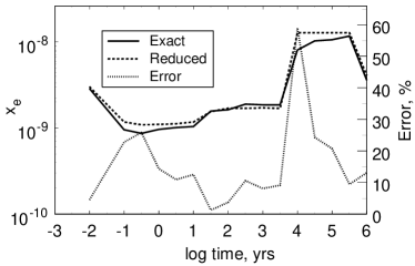
Figure 4: Evolution of the fractional ionisation in the intermediate layer at $R=3$ AU. The exact solution is shown by the solid line. The dashed line corresponds to the reduced network consisting of 112 species and 195 reactions. The dotted line (right Y-axis) shows the relative uncertainty in the fractional ionisation computed with the reduced network.

In the initial abundance set sulphur is mostly bound in CS and H₂S molecules, which are destroyed by He⁺, producing either S⁺ or S (as well as C, C⁺, and H₂). Passing through a few reactions, the most important of which is the reaction with CH₄, sulphur is reunited with carbon in a CS molecule. This process is well equilibrated, when the abundance of methane is high, and leads to a negligible S⁺ abundance at $t<10^{4}$ yrs. However, with time, some carbon atoms (both free and incorporated into CH₄) are taken out of this cycle due to formation of long carbon chains in reactions of C⁺ with methane and other hydrocarbons. After 3000 yrs the cycle is broken entirely. As the abundance of methane and other light carbon-bearing species goes down, that of ionised sulphur grows, causing almost an order of magnitude increase in the fractional ionisation.

Further evolution of $x_{\mathrm{e}}$ is implicitly controlled by gas-phase and surface reactions involving carbon chains. The reduction methods allow one to find which of them are most important, as shown in Figure 5. The main route for synthesis and destruction of long carbon chains in the depicted scheme starts with an acetylene molecule containing only two carbon atoms, which is rapidly converted to C₅H₂ molecules. This molecule then either transforms to even longer chains, or proceeds further down the cycle to C₅H⁺ which recombines to C₄H. This species starts a chain of very slow reactions with atomic oxygen that degrades it to C₃H, C₂H, and CH. Eventually, destruction of carbon chains leads to the new growth of methane abundance and to the slow decrease of the fractional ionisation. Ionised sulphur is consumed in the reaction with CH₄ and eventually is converted back to CS. The abundance of H${}_{3}^{+}$ determines the ionisation degree at the end of the computation.

Figure 5: Main routes governing synthesis and destruction of long carbon chains. Surface reactions are indicated by dashed lines.

Conversion of C₅H₂ molecules into longer chains (lower part of Figure 5) slows down the methane abundance restoration. The reduced network must include almost all species with six carbon atoms to reproduce properly the time scale of this process. Three key reactions of this carbon chain cycle proceed on dust grain surfaces. These are reactions of hydrogen addition to C₅H, C₆, and C₆H (shown with dashed lines). Without these reactions the sequence of carbon chain synthesis would be terminated by the C₅N molecule that lacks effective destruction pathways in the given conditions. Exhaustion of atomic and ionised carbon would keep the ionised sulphur at a high level, reached at $t\sim 3000$ years. Thus, we must conclude that at least within the limits of the adopted chemical model some surface reactions are of crucial significance. As far as we know, this is the first indication that the surface chemistry may have an “order-of-magnitude” importance for the evolution of fractional ionisation in interstellar matter.

4.3 Ionisation in the surface layer

The surface layer encompasses those disc regions where the degree of ionisation reaches a value of $\sim 10^{-4}$ at the end of the evolutionary time. The corresponding physical conditions imply low densities ($\rho\sim 10^{-19}-10^{-13}$ g cm^-3, moderate temperatures ($T<250$ K), a high X-ray ionisation rate and low obscuration of the UV radiation. Conditions in the surface layer are given in Table 6. Note that the temperature of the disc atmosphere is nearly constant in the vertical direction at any distance from the star. This rather extreme environment presumes a chemical evolution typical of photon-dominated regions (PDR). The chemistry is dominated by gas-phase processes, while the role of gas-grain interactions is negligible, apart from the desorption of initially abundant surface species. As our definition of the surface layer is based on the fractional ionisation value, the layer can be further divided into two chemically distinct zones. Closer to the star ($r\la 10$ AU) $x_{\mathrm{e}}$ is controlled by the X-ray ionisation, while in the outer regions ($r\ga 10$ AU) ionisation is mainly provided by the UV photons.

4.3.1 X-ray dominated chemistry

Table 6: Physical conditions in the surface layer.

$R$, AU	$\rho$, g cm-3	$T$, K	$G_{0}$	$A_{\rm V}^{\rm S}$, mag	$A_{\rm V}^{\rm IS}$, mag	$\zeta$, s-1
1	$2(-14)-1(-13)$	$\sim 180$	$1(8)$	$>10$	$\sim 1$	$2(-9)$
3	$2(-16)-1(-15)$	$\sim 230$	$7(7)$	$\sim 1.0$	$<0.5$	$8(-12)$
10	$1(-17)-8(-17)$	$140-160$	$9(5)$	$<1$	$<0.5$	$6(-13)$
30	$3(-18)-1(-17)$	$80-100$	$9(4)-1(3)$	$<1$	$<0.5$	$5(-14)$
100	$4(-19)-4(-18)$	$60-70$	$5(3)-7(3)$	$<1$	$<0.5$	$1(-15)-4(-15)$
300	$3(-19)-2(-18)$	$35-40$	$5(2)-7(2)$	$<1$	$<0.5$	$7(-17)-2(-16)$
370	$1(-19)-1(-18)$	$30-40$	$2(2)-4(2)$	$<1$	$<0.5$	$5(-17)-1(-16)$

Table 7: Reduced network for X-ray dominated chemistry in the surface layer (superscript “d” is used to denote surface species).

${\rm H}_{2}{\rm CO}^{\rm d}$	$\rightarrow$	${\rm H}_{2}{\rm CO}$
${\rm H}_{2}{\rm O}^{\rm d}$	$\rightarrow$	${\rm H}_{2}{\rm O}$
${\rm C}+h\nu_{\rm CR}$	$\rightarrow$	${\rm C}^{+}+e^{-}$
${\rm OH}+h\nu_{\rm CR}$	$\rightarrow$	${\rm O}+{\rm H}$
${\rm CO}+h\nu_{\rm CR}$	$\rightarrow$	${\rm C}+{\rm O}$
${\rm H}_{2}{\rm CO}+h\nu_{\rm CR}$	$\rightarrow$	${\rm CO}+{\rm H}_{2}$
${\rm H}+$ CRP,X-ray	$\rightarrow$	${\rm H}^{+}+e^{-}$
${\rm H}_{2}+$ CRP,X-ray	$\rightarrow$	${\rm H}_{2}^{+}+e^{-}$
${\rm H}_{2}^{+}+{\rm H}_{2}$	$\rightarrow$	${\rm H}_{3}^{+}+{\rm H}$
${\rm H}^{+}+{\rm O}$	$\rightarrow$	${\rm O}^{+}+{\rm H}$
${\rm H}^{+}+{\rm OH}$	$\rightarrow$	${\rm OH}^{+}+{\rm H}$
${\rm H}_{3}^{+}+{\rm O}$	$\rightarrow$	${\rm OH}^{+}+{\rm H}_{2}$
${\rm H}_{3}^{+}+{\rm H}_{2}{\rm O}$	$\rightarrow$	${\rm H}_{3}{\rm O}^{+}+{\rm H}_{2}$
${\rm H}_{3}^{+}+{\rm CO}$	$\rightarrow$	${\rm HCO}^{+}+{\rm H}_{2}$
${\rm O}^{+}+{\rm H}$	$\rightarrow$	${\rm H}^{+}+{\rm O}$
${\rm O}^{+}+{\rm H}_{2}$	$\rightarrow$	${\rm OH}^{+}+{\rm H}$
${\rm OH}^{+}+{\rm H}_{2}$	$\rightarrow$	${\rm H}_{2}{\rm O}^{+}+{\rm H}$
${\rm H}_{2}{\rm O}^{+}+{\rm H}_{2}$	$\rightarrow$	${\rm H}_{3}{\rm O}^{+}+{\rm H}$
${\rm C}^{+}+{\rm H}_{2}{\rm O}$	$\rightarrow$	${\rm HCO}^{+}+{\rm H}$
${\rm C}^{+}+{\rm O}_{2}$	$\rightarrow$	${\rm O}^{+}+{\rm CO}$
${\rm O}+{\rm OH}$	$\rightarrow$	${\rm O}_{2}+{\rm H}$
${\rm H}^{+}+e^{-}$	$\rightarrow$	${\rm H}+h\nu$
${\rm H}_{3}^{+}+e^{-}$	$\rightarrow$	${\rm H}_{2}+{\rm H}$
${\rm C}^{+}+e^{-}$	$\rightarrow$	${\rm C}+h\nu$
${\rm H}_{2}{\rm O}^{+}+e^{-}$	$\rightarrow$	${\rm O}+{\rm H}_{2}$
${\rm H}_{3}{\rm O}^{+}+e^{-}$	$\rightarrow$	${\rm OH}+{\rm H}+{\rm H}$
${\rm HCO}^{+}+e^{-}$	$\rightarrow$	${\rm CO}+{\rm H}$

The evolution of the ionisation degree in the hot ($T\sim 200$ K) part of the surface layer closer to the star is determined by X-ray ionisation of atomic hydrogen. The final equilibrium ionisation degree is well reproduced by the network, consisting of hydrogen-bearing species (H, H⁺, H${}_{2}^{+}$, H${}_{3}^{+}$) only. This equilibrium value is reached after 100 years of evolution. Up to this time $x_{\mathrm{e}}$ is determined by a more complicated set of chemical processes, which includes H${}_{3}^{+}$ formation, an H₃O⁺ formation and destruction cycle as well as reactions involving CO and HCO⁺. The primary carbon and oxygen carrier, formaldehyde, adds to this complexity by being desorbed from grain surfaces and destroyed by cosmic ray and X-ray induced photons. The cycles that involve these molecules are not equilibrated. Most reactions with polyatomic species tend to produce atomic hydrogen, which is gradually ionised by intense X-ray radiation. Eventually, all complex molecules are destroyed, and at the end of the computation, the gas mostly consists of atoms and atomic ions. The entire reduced network comprises 21 species and 27 reactions and is presented in Table LABEL:m1_6. The uncertainty does not exceed 60% during the entire computational time (Fig. 6). Without this simple, but important ion-molecule chemistry, the uncertainty at earlier times would be much larger (exceeding an order of magnitude).

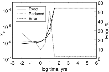
Figure 6: Evolution of the fractional ionisation in the surface layer at $R=1$ AU. The exact solution is shown with the solid line. Dashed line corresponds to the reduced network consisting of 21 species and 27 reactions. Dotted line (right Y-axis) shows the relative uncertainty in the fractional ionisation computed with the reduced network.

4.3.2 UV-dominated chemistry

The evolution of the ionisation fraction in the distant regions of the surface layer ($r\ga 10$ AU) is similar but more complicated from the chemical point of view than in the case of the X-ray dominated chemistry. As the intensity of stellar X-rays decreases, UV photons become the main ionising source (see Table 6). The typical gas temperature in this part of the disc decreases below $100$ K. The entire ionisation evolution of the region is determined by formaldehyde desorption and destruction. Icy mantles illuminated by UV radiation evaporate, thus delivering H₂CO into the gas phase. This molecule is either destroyed directly by photons (H${}_{2}\mathrm{CO}\rightarrow\mathrm{CO,HCO}^{+}$) or ionised and dissociated (H${}_{2}\mathrm{CO}\rightarrow\mathrm{H}_{2}\mathrm{CO}^{+}\rightarrow\mathrm{CO}$). HCO⁺ dissociatively recombines to CO as well, and this molecule is dissociated by photons producing C and O. The destruction processes proceed very fast, so after only a fraction of a year the gas composition is mostly atomic, with C⁺ being the dominant ion. When all polyatomic species are destroyed, the fractional ionisation is regulated by an equilibrium ionisation-recombination cycle of atomic carbon. The reduced network consisting of less than 15 species and about 20 reactions leads to less than 20% uncertainty during the entire computational time. An example of such a network for $R=100$ AU is given in Table 8.

Table 8: Reduced network for UV-dominated chemistry in the surface layer.

${\rm H}_{2}{\rm CO}^{\rm d}$	$\rightarrow$	${\rm H}_{2}{\rm CO}$
${\rm C}^{+}+{\rm H}_{2}{\rm CO}$	$\rightarrow$	${\rm H}_{2}{\rm CO}^{+}+{\rm C}$
${\rm C}^{+}+e^{-}$	$\rightarrow$	${\rm C}+h\nu$
${\rm HCO}^{+}+e^{-}$	$\rightarrow$	${\rm CO}+{\rm H}$
${\rm H}_{2}{\rm CO}^{+}+e^{-}$	$\rightarrow$	${\rm CO}+{\rm H}+{\rm H}$
${\rm H}_{2}{\rm CO}^{+}+e^{-}$	$\rightarrow$	${\rm H}_{2}{\rm CO}+h\nu$
${\rm C}+h\nu$	$\rightarrow$	${\rm C}^{+}+e^{-}$
${\rm CO}+h\nu$	$\rightarrow$	${\rm C}+{\rm O}$
${\rm H}_{2}{\rm CO}+h\nu$	$\rightarrow$	${\rm CO}+{\rm H}_{2}$
${\rm H}_{2}{\rm CO}+h\nu$	$\rightarrow$	${\rm CO}+{\rm H}+{\rm H}$
${\rm H}_{2}{\rm CO}+h\nu$	$\rightarrow$	${\rm H}_{2}{\rm CO}^{+}+e^{-}$
${\rm H}_{2}{\rm CO}+h\nu$	$\rightarrow$	${\rm HCO}^{+}+e^{-}+{\rm H}$

5 Column densities

A useful product of our study is the complete chemical structure of the disc. We present the calculated column densities of some species along with observed values and column densities obtained by other groups in Table 9. The observed values are taken from Aikawa et al. (warm (2002)), Table 1. Five theoretical models of the chemical evolution of a protoplanetary disc are considered. The main differences between them are discussed below.

Willacy & Langer (wl00 (2000)) used the gas-phase UMIST 95 database, supplied with an additional set of gas-grain processes and surface reactions. They adopted an extrapolated flared T Tau disc model of Chiang & Goldreich (CG97 (1997)), taking into account cosmic rays and stellar UV radiation and assuming a sticking probability $S=1$. In all the other models, namely, in Aikawa & Herbst (ah1999 (1999, 2001)), Aikawa et al. (warm (2002)), and van Zadelhoff et al. (vzdetal (2003)), the New Standard Model (NSM) with a set of gas-grain interaction processes is used as the chemical network.

Aikawa & Herbst (ah1999 (1999, 2001)) considered an extrapolated minimum-mass solar nebula model of Hayashi (mmsn (1981)), taking into account stellar X-ray radiation in addition to the UV radiation and cosmic rays and assuming an artificially low sticking probability $S=0.03$ that compensates for the absence of non-thermal desorption mechanisms. The flared T Tau disc model of D’Alessio et al. (DALdisc (1999)) for various accretion rates is used with a sticking probability $S=1.0$ in Aikawa et al. (warm (2002)) and van Zadelhoff et al. (vzdetal (2003)). Stellar X-rays are not included in the latter two models.

Table 9: The observed and calculated column densities in cm^-2, $r=370$ AU, $t=10^{6}$ yrs.

Species	I	II	III	IV	V	This paper		Observed			Max.
						$\dot{M}$, $M_{\odot}$ yr-1		DM Tau	LkCa15∗	LkCa15∗∗	difference
						$10^{-9}$	$10^{-7}$	(SD)	(IM)	(SD)
H2	9(22)	9(21)	$1.5(24)$	$1.3(22)$	1.3(23)	$4.8(21)$	$1.4(24)$	$3.8(21)$	—	—
H2O	—	—	—	2.7(14)	8.0(13)	$2.1(14)$	$1.6(14)$	—	—	—	$\sim 3$
HCN	2(12)	2(12)	2.1(12)	1.4(12)	2.5(12)	$1.3(13)$	$6.7(12)$	$2.1(12)$	$0.02-1.2(15)$	$7.8(13)$	$\sim 10$
NH3	—	1(13)	—	1.4(13)	—	$4.4(13)$	$1.4(14)$	—	—	—	$\sim 15$
C2H	2(12)	8(12)	6.2(12)	8.9(11)	2.0(13)	$7.0(12)$	$1.1(13)$	$4.2(13)$	—	—	$\sim 20$ (10)
HNC	1(12)	—	2.0(12)	3.0(11)	—	$6.9(12)$	$8.0(12)$	$9.1(11)$	$<5.4(12)$	—	$\sim 30$ (8)
CN	1(13)	1(13)	3.8(12)	5.3(11)	3.0(13)	$6.4(12)$	$4.6(12)$	$9.5-12(12)$	$9.1-25(13)$	$6.3(14)$	$\sim 60$ (8)
N2H+	—	—	1.9(12)	8.1(11)	—	$6.0(12)$	$8.1(13)$	$<7.6(11)$	$<5.7(12)$	$<5.9(13)$	$\sim 100$ (40)
HCO+	3(11)	5(11)	$9.0(12)$	8.8(10)	9.0(12)	$8.4(11)$	$2.0(11)$	$4.6-28(11)$	$1.5(13)$	$1.4(13)$	$\sim 100$ (45)
CS	3(11)	1(12)	$4.9(11)$	1.0(11)	1.2(12)	$5.6(12)$	$1.1(13)$	$6.5-13(11)$	$1.9-2.1(13)$	$2.2(14)$	$\sim 110$ (35)
CO	2(15)	8(15)	$1.1(18)$	7.1(16)	1.2(18)	$1.6(16)$	$2.5(16)$	$5.7(16)$	$1.6(18)$	$9.0(17)$	$\sim 600$
H2CO	7(11)	1(12)	$2.9(12)$	8.7(10)	—	$8.0(13)$	$8.3(13)$	$7.6-19(11)$	—	$3.0-22(13)$	$\sim 10^{3}$
CH3OH	—	—	$6.4(08)$	7.7(11)	—	$4.0(10)$	$2.9(10)$	—	$7.3-18(14)$	$<9.4(14)$	$<10^{3}$

• Aikawa & Herbst (1999), Fig. 7, $R=400$ AU, $t=9.5\cdot 10^{5}$ yrs, high $\zeta$ case

• Aikawa & Herbst (2001), Fig. 6, $R=400$ AU, $t=9.5\cdot 10^{5}$ yrs

• Aikawa et al. (warm (2002)), Table 1, $\dot{M}=10^{-7}\,M_{\odot}$ yr^-1, $R=370$ AU, $t=9.5\cdot 10^{5}$ yrs

• Willacy & Langer (2000), Table 4, interpolated to $R=400$ AU, $t=10^{6}$ yrs

• van Zadelhoff et al. (vzdetal (2003)), Fig. 5, $R=400$ AU

• interferometric observations, beam size is $\sim 4\arcsec$

• single-dish observations, beam size is $\sim 20\arcsec$

• do not necessarily correspond to $r=370$ AU,

• disc size is $\sim 100$ AU

Column densities of selected species presented in these papers are compared to those computed in this work in Table 9. Wherever possible, we took values from tables, otherwise figures were used. Throughout this paper, a disc model with an accretion rate of $10^{-7}\,M_{\odot}$ yr^-1 is used, but in Table 9 we also present results of time-dependent chemical models for a lower accretion rate, $\dot{M}=10^{-9}\,M_{\odot}$ yr^-1.

To characterise differences between model predictions, we divide all species in three groups by the maximum ratio of their theoretical column densities (less than 20, less than 200, and the rest). Given the wide variety of conditions and assumptions made in the various models, it is natural to expect that differences in calculated column densities should be significant. However, in reality, column densities for many species are close to each other in the different studies. For example, the scatter in HCN column densities does not exceed an order of magnitude. Similarly, ammonia densities in all but one case are a few times $10^{13}$ cm^-2. Note that we omitted the anomalously high NH₃ column density computed by Aikawa & Herbst (ah1999 (1999)) as this was based on an unrealistic rate for the H${}_{3}^{+}+\mathrm{N}$ reaction (Aikawa & Herbst ah2001 (2001)).

Somewhat higher maximum-to-minimum ratios for species in the second group are mainly caused by their low abundances in the Willacy & Langer (wl00 (2000)) model. In the last column of Table 9 we give relative variations of their column densities both with and without (in parentheses) Willacy & Langer (wl00 (2000)) data. If the latter are not taken into account, the ratio of maximum to minimum column density does not exceed 50 for all these molecules. This similarity of column densities and a lack of correlation between them and the column density of molecular hydrogen can be understood as a further manifestation of the “warm molecular layer” (Aikawa et al. warm (2002)) where nearly all admixture gas-phase molecules are concentrated. On the other hand, molecular hydrogen is concentrated in the midplane, where all other molecules are frozen out and thus do not contribute to column densities.

The reason why column densities in the calculations of Willacy & Langer are lower in comparison with other studies is probably related to the disc model they adopted. In the model of Chiang & Goldreich (CG97 (1997)) the disc is assumed to consist of only two layers, namely, the dark dense midplane and the less dense surface layer subject to harsh UV radiation. In the cold midplane molecules are mainly locked in icy mantles while in the surface layer they are easily dissociated or ionised by UV photons. In contrast to the disc model of D’Alessio et al. (DALdisc (1999)), there is no region similar to the shielded intermediate (“warm molecular”) layer, which is the most favourable disc domain for many molecules to have their maximum gas-phase concentrations.

The most striking finding is variations in theoretical CO column densities. As carbon monoxide, like other molecules, has its highest abundance in the intermediate layer, we might expect that its abundance is relatively independent of the total gas column density. Thus, the origin of the large discrepancies in CO abundances should lie in physical differences between various models. Looking at Table 9, one is tempted to assume that the CO abundance is low in models with surface chemistry (this paper and Willacy & Langer wl00 (2000)) or in models with X-ray induced chemistry (this paper and Aikawa & Herbst ah1999 (1999, 2001)). In the former case the CO molecule might be transformed to CO₂ and H₂CO, in the latter case it might be destroyed by abundant He⁺.

To check if this is the case, we computed the vertical distribution of CO for $R=370$ AU without surface reactions and with $\zeta_{\mathrm{X}}$=0. In both cases we failed to reproduce the high CO column densities obtained by Aikawa et al. (warm (2002)) and van Zadelhoff et al. (vzdetal (2003)). As we noted above, the low CO column density in the Willacy & Langer model can partly be caused by the disc model they adopted. A possible explanation for the low CO abundance in our model is the fact that we do not take into account self- and mutual-shielding of molecular hydrogen and carbon monoxide, contrary to Aikawa et al. (warm (2002)) and Zadelhoff et al. (vzdetal (2003)).

In addition, we include in Table 9 observationally inferred column densities for DM Tau (single-dish measurements) and LkCa15 (interferometric data). Note that DM Tau values correspond to column densities averaged over the entire disc ($\sim 800$ AU), while values estimated from LkCa15 single-dish observations are column densities averaged over a $\sim 100$ AU disc. For species in the first and second groups there is a reasonable agreement between our predictions and observational data.

6 Discussion

Recent theoretical studies (e.g. Aikawa & Herbst ah1999 (1999, 2001), Aikawa et al. warm (2002), van Zadelhoff et al. vzdetal (2003)) revealed that the distribution of gas-phase molecular abundances within a steady-state accretion disc in the absence of mixing processes has a three-layer vertical structure. In the dense and cold midplane all species, except the most volatile ones, are frozen out on grain surfaces while in the disc atmosphere (surface layer) they are easily destroyed by high-energy stellar radiation. Therefore, in these disc domains gas-phase abundances of polyatomic species are low. On the contrary, in the intermediate layer, which is shielded from UV photons but still warm enough to allow effective desorption, most molecules remain in the gas phase and drive a complex chemistry resulting in a rich molecular composition. As we noted above, this simple picture may not be appropriate when diffusion processes are taken into account (Ilgner et al. IHMM03 (2003)).

In our study we focused on the analysis of chemical processes relevant to the evolution of disc fractional ionisation based on the reduction approach. The size of a reduced chemical network, accurately reproducing the electron concentration in a given disc region, can be understood as a quantitative criterion for the complexity of ionisation chemistry. In Figure 7 we show the distribution of the number of species in the reduced networks over the disc. This distribution demonstrates a layered pattern. In most parts of the disc the chemistry of ionisation is simple either due to the lack of ionising factors, low temperature and high density (midplane) or due to the presence of ionising radiation (surface layer). In these regions, it is sufficient to keep about 10–30 species and a few tens of reactions in reduced networks. Between the midplane and the surface layer the intermediate layer is located, where the evolution of ionisation degree is more complicated from the chemical point of view (especially at early times). Here, one has to retain more than fifty species and a comparable number of reactions in the reduced networks.

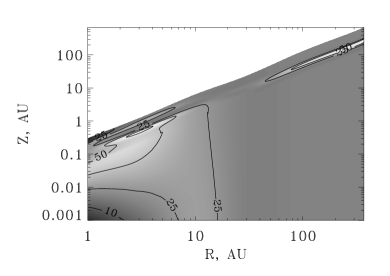
Figure 7: The distribution of the number of species in the reduced networks governing fractional ionisation over the disc. The highest and smallest number of species is 112 and 5, respectively.

This layered structure is directly related to the size and location of the so-called “dead zone” within a protoplanetary disc, which is the region where the ionisation degree is so low that the magnetic field is not coupled to the gas. The MHD turbulence cannot develop in this region. Thus, the MRI is not operative, which means the lack of an effective angular momentum transport if no other transport mechanism can be identified. The “dead zone” in accretion discs has been widely investigated (e.g. Igea & Glassgold  IG99 (1999), Fromang et al. from2002 (2002), Sano et al. sano (2000)).

An important quantity which characterises the coupling between the matter and the magnetic field is the magnetic Reynolds number, which can be defined as (Fromang et al. from2002 (2002))

$$Re_{M}=\frac{c_{s}H}{\eta},$$ (7)

where $\eta$ is the Ohmic resistivity (Blaes & Balbus bb1994 (1994))

$$\eta=\frac{234\cdot T^{0.5}}{x_{\mathrm{e}}}.$$ (8)

The other quantities are the sound speed $c_{s}$, and the thickness of the disc $H$. The MHD turbulence can be maintained only if this quantity exceeds a certain critical value which depends on the field geometry and other factors. Following Fromang et al., we consider two cases of this limiting value, namely, $Re_{M}^{\mathrm{crit}}=100$ and $Re_{M}^{\mathrm{crit}}=1$ and define the “dead zone” as a disc domain where $Re_{M}<Re_{M}^{\mathrm{crit}}$.

The calculated magnetic Reynolds numbers for our model are shown in Fig. 8. The lowest magnetic Reynolds number is $Re_{M}\sim 10$, which implies that under certain circumstances within the framework of our model the “dead zone” is entirely absent. With another critical value, $Re_{M}^{\mathrm{crit}}=100$, the “dead zone” occupies the following disc region: $2\leavevmode\nobreak\ \mathrm{AU}<r<20$ AU, $z\sim 0.06\cdot r^{1.27}$ (solid line). This result is roughly consistent with other recent studies. For example, Fromang et al. found that the “dead zone” can extend over $0.7\leavevmode\nobreak\ \mathrm{AU}<r<100$ AU, if the viscosity parameter is equal to $10^{-2}$ and the accretion rate is $10^{-7}\,M_{\odot}$ yr^-1, whereas Igea & Glassgold (IG99 (1999)) obtained a “dead zone” of somewhat smaller size, $r<5$ AU.

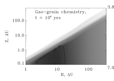
Figure 8: The magnetic Reynolds numbers computed for our model and an evolutionary time of $10^{6}$ yrs. The solid line designates $Re_{M}^{\mathrm{crit}}=100$. The highest and lowest values are equal to about $10^{13}$ and 10, respectively.

Apart from defining the location of the “dead zone” in accretion discs, the fractional ionisation determines whether non-ideal MHD effects are important for the evolution of protoplanetary discs. When the electron abundance is computed for the solution of non-ideal MHD equations, an ionisation equilibrium is often assumed. An expression similar to Eq. (1) is then used to calculate the equilibrium fractional ionisation, with different estimates for the gas-phase recombination coefficient $\beta$ (Blaes & Balbus bb1994 (1994); Gammie gammie (1996); Regos regos (1997); Reyes-Ruiz rr2001 (2001); Fromang et al. from2002 (2002); Fleming & Stone fs2003 (2003)).

In Fig. 9 we compare the fractional ionisation $x_{\mathrm{e}}(\mathrm{eq})$, computed from Eq. (1) with the often used expression for recombination coefficient $\beta=8.7\cdot 10^{-6}T^{-1/2}$ (Glassgold, Lucas, & Omont beta1986 (1986)), to the fractional ionisation computed with the full chemical network $x_{\mathrm{e}}(\mathrm{full})$, for some representative points in the midplane and in the intermediate layer. It is not surprising that the ratio of these two quantities exceeds 10 at low ionisation degrees. Here the electron density is small and ion-grain interactions should be taken into account. At moderate ionisation degrees ($10^{-10}-10^{-8}$), the equilibrium value may differ from the “exact” value by a factor of a few at the end of the computation. At earlier times, the discrepancy is higher.

However, in the midplane the equilibrium state is reached very rapidly, with no appreciable changes in $x_{\mathrm{e}}$ after $\sim 1000$ years of evolution. If one is not interested in time scales less than 1000 years and can afford a factor of a few uncertainty in the fractional ionisation, deep in the disc interior the equilibrium $x_{\mathrm{e}}$ is sufficient, provided grain charging processes are taken into account.

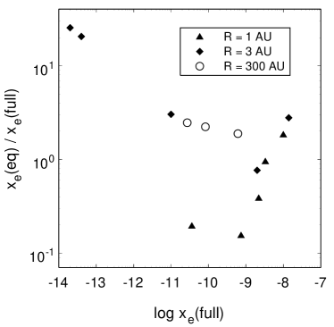
Figure 9: Comparison of the equilibrium and time-dependent fractional ionisations at $t=10^{6}$ years in the midplane and in the intermediate layer. Symbols correspond to different radii.

The intermediate layer shows a very different behaviour. As we mentioned previously, the equilibrium state is not reached there or is reached very late. The initial fall-off of $x_{\mathrm{e}}$, caused by HCO⁺, H${}_{3}^{+}$ and metal ion recombination, is followed by a step-like increase. The duration of each phase and $x_{\mathrm{e}}$ evolutionary changes, illustrated in Figure 4, vary significantly in different parts of the layer. Surprisingly, the equilibrium $x_{\mathrm{e}}$ from Eq. (1) is very close to the computed fractional ionisation at $t=10^{6}$ years in this point ($1.5\cdot 10^{-9}$ and $2\cdot 10^{-9}$, respectively). This is, of course, a coincidence, as the equilibrium is not reached there. We emphasise that even if $x_{\mathrm{e}}$(full) is equilibrated eventually in the intermediate layer and is close to $x_{\mathrm{e}}$(eq), the latter value does not reflect the ionisation state of the medium for most of the computational time.

In the surface layer the fractional ionisation is controlled not only by X-rays, but also by UV-radiation. The equation (1) is still applicable here but with an important change. In the surface layer $x_{\mathrm{e}}$ is determined mostly by ionised carbon (Table 1). Its recombination coefficient is much lower than the value quoted above, thus, $\beta=8.7\cdot 10^{-6}T^{-1/2}$ should not be used in this case. If one substitutes in Eq. (1) the correct $\beta$ for C⁺ ($1.4\cdot 10^{-13}T^{-0.61}$), the resultant equilibrium $x_{\mathrm{e}}$ is a few times smaller than the “exact” value, mainly because photoionisation is not taken into account. Time needed to reach the equilibrium $x_{\mathrm{e}}$ in the surface layer does not exceed 100 years. It is questionable whether precise information about such a high ionisation ($x_{\mathrm{e}}\sim 10^{-4}$) is required for MHD computation.

Overall, we conclude that the equilibrium approach is appropriate most of the time and in most parts of the studied disc, but it should be applied with care. This is especially important in less dense discs that are more transparent to X-rays and UV radiation. In this paper, we used a relatively massive disc model with a narrow intermediate layer. In models with lower accretion rates the intermediate layer would occupy a greater volume of the disc.

Even though the reduced networks presented in this paper provide much better accuracy than the equilibrium approach, while having quite modest sizes, their usefulness for dynamical models is limited by the fact that they are computed in a steady-state disc. For example, in the point M1 the reduced network consists of three species, NO, Mg, and Mg⁺. This network is of no use in a dynamical model because there will be no NO in the gas flowing into the inner part of the midplane, as reduced networks further out in the midplane do not contain this molecule. To make the reduction valuable for MHD modelling we need to consider it in a dynamically evolving medium.

An alternative approach is to merge all the networks described in this paper into a single network that comprises about 120 species and a comparable number of reactions. This network is out of the scope of the present paper and will be described in further publications.

7 Conclusion

Chemical processes, responsible for the ionisation structure of a protoplanetary disc with a central star, are analysed by means of reduced networks that reproduce the ionisation fraction within a factor of 2. These networks are available from the authors upon request. Because of the wide range of physical conditions met in a typical disc, there is a corresponding diversity in the chemical reactions that control the fractional ionisation in different parts of the disc. Generally, it can be divided into three layers. In the midplane the ionisation is provided by cosmic rays and radioactive elements only. Above the midplane, the intermediate layer is located where the ionisation is dominated by X-rays. In the surface layer UV photons are the main ionising factor. In each of these layers we analyse several representative points and construct reduced chemical networks that are needed to reproduce the fractional ionisation as a function of time during $10^{6}$ years of evolution within a factor of 2 uncertainty. In the midplane the chemistry, which determines the fractional ionisation, is very simple. Reduced networks typically include no more than 10 species and a similar number of reactions. The same holds true for the surface layer. The intermediate layer is the most complicated region from the chemical point of view. To compute the fractional ionisation with the targeted accuracy, in some regions one has to take into account carbon chains containing up to 6 carbon atoms, which leads to reduced networks with over a hundred species and reactions.

- (1) Aikawa, Y., & Herbst, E. 1999, A&A, 351, 233
- (2) Aikawa, Y., & Herbst, E. 2001, A&A, 371, 1107
- (3) Aikawa, Y., van Zadelhoff, G. J., van Dishoeck, E. F., Herbst, E. 2002, A&A, 386, 622
- (4) Balbus, S. A., & Hawley, J. F. 1991, ApJ, 376, 214
- (5) Bauer, I., Finocchi, F., Duschl, W. J., Gail, H.-P., Schloeder, J. P. 1997, A&A, 317, 273
- (6) Blaes, O. M., & Balbus, S. A. 1994, ApJ, 421, 163
- (7) Burke, J. R., & Hollenbach, D. 1983, ApJ, 265, 223
- (8) Chiang, E., & Goldreich, P. 1997, ApJ, 490, 368
- (9) D’Alessio, P., Calvet, N., Hartmann, L., Lizano, S., Canto, J. 1999, ApJ, 527, 893
- (10) Draine, B. T. 1978 ApJS, 36, 595
- (11) Fleming, T., & Stone, J. 2003, ApJ, 585, 908
- (12) Fromang, S., Terquem, C., Balbus, S. A. 2002, MNRAS, 329, 18
- (13) Gammie, Ch. 1996, ApJ, 457, 355
- (14) Glassgold, A. E., Lucas, R., & Omont, A. 1986, A&A, 157, 35
- (15) Glassgold, A. E., Najita, J., Igea, J. 1997a, ApJ, 480, 344
- (16) Glassgold, A. E., Najita, J., Igea, J. 1997b, ApJ, 485, 920
- (17) Hasegawa, T. I., Herbst, E., & Leung, C. M. 1992, ApJS, 82, 167
- (18) Hasegawa, T. I., & Herbst, E. 1993, MNRAS, 263, 589
- (19) Hayashi, C. 1981, Prog. Theor. Phys., 70, 35
- (20) Igea, J., & Glassgold, A. E. 1999 ApJ, 518, 848
- (21) Ilgner, M., Henning, Th., Markwick, A., Millar, T. 2003, A&A, in press
- (22) Langer, W. D., Velusamy, T., Kuiper, T. B. H., Peng, R., McCarthy, M. C., et al. 1997, ApJ, 480, L63
- (23) Léger, A., Jura, M., Omont, A. 1985, A&A, 144, 147
- (24) Markwick, A. J., Ilgner, M., Millar, T. J., & Henning, Th. 2002, A&A, 385, 632
- (25) Millar, T. J., Farquhar, P. R. A., & Willacy, K. 1997, A&AS, 121, 139
- (26) Nishi, R., Nakano, T., Umebayashi, T. 1991, ApJ, 369, 181
- (27) Ohishi, M., Irvine, W. M., & Kaifu, N. 1992, in Astrochemistry of Cosmic Phenomena, ed. P. D. Singh (Dordrecht: Kluwer), 171
- (28) Oppenheimer, M., & Dalgarno, A. 1974, ApJ, 192, 29
- (29) Roberts, H., Herbst, E. 2002, A&A, 395, 233
- (30) Regos, E. 1997, MNRAS, 286, 97
- (31) Reyes-Ruiz, M. 2001, ApJ, 547, 465
- (32) Ruffle, D. P., Rae, J. G. L., Pilling, M. J., Hartquist, T. W., & Herbst, E. 2002, A&A, 381, L13
- (33) Sano, T., Miyama, Sh. M., Umebayashi, T., & Nakano, T. 2000, ApJ, 543, 486
- (34) Terzieva, R., Herbst, E. 1998a, ApJ, 501, 207
- (35) Terzieva, R., Herbst, E. 1998b, ApJ, 509, 932
- (36) Umebayashi, T., & Nakano, T. 1980, PASJ, 32, 405
- (37) van Zadelhoff, G.-J., Aikawa, Y., Hogerheijde, M. R., & van Dishoeck E. F. 2003, A&A, 397, 789
- (38) Walmsley, C. M., Pineau des Forêts, G., & Flower, D. R. 1999, A&A, 342, 542
- (39) Westley, M. S., Baragiola, R. A., Johnson, R. E., Baratta, G. A. 1995, Nature, 373, 405
- (40) Wiebe, D., Semenov, D., & Henning, Th. 2003, A&A, 399, 197 (Paper I)
- (41) Willacy, K., Klahr, H. H., Millar, T. J., Henning Th. 1998, A&A, 338, 995
- (42) Willacy, K., Langer, W. 2000, A&A, 397, 789