An Extended Scheme for Fitting X-ray Data with Accretion Disk Spectra in the Strong Gravity Regime^†

Abstract

Accreting black holes are believed to emit X-rays which then mediate information about strong gravity in the vicinity of the emission region. We report on a set of new routines for the xspec package for analysing X-ray spectra of black-hole accretion disks. The new computational tool significantly extends the capabilities of the currently available fitting procedures that include the effects of strong gravity, and allows one to systematically explore the constraints on more model parameters than previously possible (for example black-hole angular momentum). Moreover, axial symmetry of the disk intrinsic emissivity is not assumed, although it can be imposed to speed up the computations. The new routines can be used also as a stand-alone and flexible code with the capability of handling time-resolved spectra in the regime of strong gravity. We have used the new code to analyse the mean X-ray spectrum from the long XMM–Newton 2001 campaign of the Seyfert 1 galaxy MCG–6-30-15. Consistent with previous findings, we obtained a good fit to the broad Fe K line profile for a radial line intrinsic emissivity law in the disk which is not a simple power law, and for near maximal value of black hole angular momentum. However, equally good fits can be obtained also for small values of the black hole angular momentum. The code has been developed with the aim of allowing precise modelling of relativistic effects. Although we find that current data cannot constrain the parameters of black-hole/accretion disk system well, the code allows, for a given source or situation, detailed investigations of what features of the data future studies should be focused on in order to achieve the goal of uniquely isolating the parameters of such systems.

1 Introduction

There is now strong evidence that the Fe K$\alpha$ line emission in some active galactic nuclei (AGN) and some Galactic X-ray binary black-hole candidates (BHC) originates, at least in part, from an accretion disk in a strong gravitational field. A lively debate is aimed at addressing the question of what the spectral line profiles and the associated continuum can tell us about the central black-hole, and whether they can be used to constrain parameters of the accretion disk in a nearby zone, about ten gravitational radii or less from the center. For a recent review for AGNs, see Fabian et al. (2000), Reynolds & Nowak (2003), and references cited therein. For BHCs, see Miller et al. (2002a), McClintock & Remillard (2003) and references therein. In several sources there is indication of Fe K$\alpha$ line emission from within the last stable orbit of a Schwarzschild black hole (e.g. in the Seyfert galaxy MCG–6-30-15; see Iwasawa et al. 1996; Fabian et al. 2000; Wilms et al. 2001; Martocchia, Matt & Karas 2002a) while in other cases the emission appears to arise farther from the black hole (e.g. in the microquasar GRS 1915+105, see Martocchia et al. 2002b; for AGNs, see Yaqoob & Padmanabhan 2004 and references therein). Often, the results from X-ray line spectroscopy are inconclusive, especially in the case of low spectral resolution data. For example, a spinning black hole is allowed but not required by the line model of the microquasar V4641 Sgr (Miller et al. 2002b). The debate still remains open, but there are good prospects for future X-ray astronomy missions to be able to use the Fe K$\alpha$ line to probe the space-time in the vicinity of a black hole, and in particular to measure the angular momentum, or the spin, associated with the metric.

One may also be able to study the ‘plunge region’ (about which very little is known), between the event horizon and the last stable orbit, and to determine if any appreciable contribution to the Fe K$\alpha$ line emission originates from there (Reynolds & Begelman 1997; Krolik & Hawley 2002). In addition to the Fe K lines, there is some evidence for relativistic soft X-ray emission lines due to the Ly$\alpha$ transitions of oxygen, nitrogen, and carbon (e.g. Mason et al. 2003), although the observational support for this interpretation is still controversial (e.g. Lee et al. 2001).

With the greatly enhanced spectral resolution and throughput of future X-ray astronomy missions, the need arises for realistic theoretical models of the disk emission and computational tools that are powerful enough to deal with complex models and to allow actual fitting of theoretical models to observational data. It is worth noting that some of the current data have been used to address the issue of distinguishing between different space-time metrics around a black hole, however, the current models available for fitting X-ray data are subject to various restrictions which we shall elaborate on in the present paper.

In this paper we describe a generalised scheme and a code which can be used with the standard X-ray spectral fitting package, xspec (Arnaud 1996). We have in mind general relativity models for black-hole accretion disks. Apart from a better numerical resolution, the principal innovations compared to currently available schemes are that the new model allows one to (i) fit for the black-hole spin, (ii) study the emission from the plunge region, and (iii) specify a more general form of emissivity as a function of polar coordinates in the disk plane (both for the line and for the continuum). Furthermore, it is also possible to (iv) study time variability of the observed signal and (v) compute Stokes parameters of a polarized signal. Items (i)–(iii) are immediately applicable to current data and modelling, while the last two mentioned features are still mainly of theoretical interest at present. Time-resolved analysis and polarimetry of accretion disks are directed towards future applications when the necessary resolution and the ability to do polarimetry are available in X-rays. Thus our code has the advantage that it can be used with time-resolved data for reverberation studies of relativistic accretion disks (Stella 1990; Reynolds et al. 1999; Ruszkowski 2000; Goyder & Lasenby 2004). Also polarimetric analysis can be performed, and this will be extremely useful because it can add very specific information on strong-gravitational field effects (Connors, Stark & Piran 1980; Matt, Fabian & Ross 1993; Bao et al. 1997). Theoretical spectra with temporal and polarimetric information can be analysed with the current version of our code and such analysis should provide tighter constrains on future models than is currently possible.

As mentioned above, Fe K lines have been reported in the X-ray spectra of numerous AGNs and BHCs. These sources frequently exhibit remarkable variability patterns which are still difficult to understand. Among these puzzling objects, the Seyfert 1 galaxy MCG–6-30-15 is radically distinctive with its broad and skewed Fe K$\alpha$ feature that persists in observations in spite of substantial variablity of the continuum. Interpretation of the Fe K line in terms of reflection from a relativistic black-hole disk has been found to be rather robust, but it has not been possible to fully explore the model parameter space. In particular, constraints on $a$ have only been obtained by fitting ‘inverted photon data’ which is made from the real data in a model-dependent way that already assumes a certain value of $a$. The puzzling stability of this line has been attributed, amongst other things, to general relativity effects very close to the black hole (Miniutti et al. 2003; Fabian & Vaughan 2003). It is thus interesting to know if and how a generalisation of the standard disk-line scheme together with accurate computation of general relativistic effects can add new pieces of information or whether a more substantial modification of the whole picture is needed (for further discussion and references, see e.g. Weaver & Yaqoob 1998; Krolik 1999; Hartnoll & Blackman 2001; Dumont et al. 2002). Different kinds of such generalisations have been proposed. Previous papers indicated that details of the model do matter. However, a strong gravitational field has almost invariably been required. In the present paper, we adopt the assumption that the line and continuum emission are produced by an irradiated disk near a rotating black hole, we relax some of the previous assumptions, and we search for best-fitting parameters of the model.

In the § 2 we describe the main features of the new computational tool. We list several variants of the code which address different problems of fitting X-ray spectra of black hole plus accretion disk systems. In § 3 we use the code to analyse time-averaged data for MCG–6-30-15 XMM–Newton CCD data as detailed in Fabian et al. 2002). We point out that more complex models may not require a large value of the black-hole angular momentum, although the current data are consistent with a maximally rotating black hole. Finally, in § 4, we summarise our results and state our conclusions.

Table 1: Basic features of the new model in comparison with other black hole disk-line models.

Model	Effects that are taken into account				Reference
	Energy shift of photons/Lensing effect	Black hole angular momentum	Axisymmetry is assumed	Steady source is assumed
diskline	yes/no	$0$	yes	yes	Fabian et al. (1989)
laor	yes/yes	$0.998$	yes	yes	Laor (1991)
kerrspec	yes/yes	$\langle 0,1\rangle^{{\dagger}}$	no	yes	Martocchia et al. (2000)
ky	yes/yes	$\langle 0,1\rangle$	no‡	no	This paper

^† The value of dimension-less $a$ parameter is kept frozen.
^‡ A one-dimensional version is available for the case of an axisymmetric disk. In this axisymmetric mode, ky still allows $a$ and other relevant parameters to be fitted (in which case the computational speed of ky is then comparable to laor). The results can be more accurate than those obtained with other routines because of the ability to tune the grid resolution.

Table 2: Basic versions of the model.

Name	Type†	Usage
KYGline	additive	Relativistic spectral line from a black hole disk.
KYHrefl	additive	Compton reflection with an incident power-law (or a broken power-law) continuum.
KYLcr	additive	Lamp-post Compton reflection model.
KYSpot	To be used as an independent code outside xspec	Time-dependent spectrum of a pattern co-orbiting with the disk.
KYConv	convolution	Convolution of the relativistic kernel with intrinsic emissivity across the disk.

^† Different model types correspond to xspec syntax and are defined by the way they act in the overall model and form the final spectrum. According to the usual convention in xspec, additive models represent individual emission spectral components which may originate e.g. in different regions of the source. Additive models are simply superposed in the total signal. Multiplicative components (e.g. hrefl, discussed in the Appendix B) multiply the current model by an energy-dependent factor. Convolution models modify the model in a more non-trivial manner. See Arnaud (1996) for details.

2 Computational Technique

The new model, ky, is suited for use with the xspec package (Arnaud 1996). Several mutations of ky were developed, with an eye to specifically provide different applications, and linked with a common ray-tracing subroutine, which therefore does not have to be touched when the intrinsic (local) emissivity function in the model is changed.

When the relativistic line distortions are computed, the new model is more accurate than the laor model (Laor 1991) and faster than kerrspec (Martocchia, Karas & Matt  2000). These are the other two xspec models with a similar usage (see also Pariev & Bromley 1998; Gierliński, Maciolek-Niedzwiecki & Ebisawa 2001; Schnittman & Bertschinger 2003). It is also important to compare the results from fully independent relativistic codes since the calculations are sufficiently complex that significant differences can arise. Our code is more general than the currently available alternatives in xspec, so it can be used to assess the shortcomings of the available codes. We compared calculated profiles of the relativistic line in our model with several models available in literature. In particular, our time-averaged profiles are in perfect agreement with those shown in Beckwith & Done (preprint, 2004). Small (but potentially significant) distinctions from other models can be explained by omission of light-focusing effect in diskline and by insufficient resolution in the laor model. The discrepancies become more prominent in extreme situations of large inclination and/or very narrow ring. Furthermore, as discussed in the text below, various uncertainties in the form of intrinsic emissivity and especially in the darkening law introduce changes in spectrum which could not be examined by older models. For more comparisons see Appendix A.

As far as the continuum component is concerned, an approximation was adopted in order to account for Compton reflection. To this end, we employ a more basic approach than the pexrav model (Magdziarz & Zdziarski 1995). Simplicity of the adopted scheme affords a much higher computation speed than other Compton reflection models in xspec. Further details of the method and the calculations for the ray-tracing are given in Appendix A, and details of the Compton reflection model we use are given in Appendix B (see also Dovčiak et al. 2004).

Among its useful features, the ky model allows one to fit various parameters such as black-hole angular momentum ($a$), observer inclination angle relative to the disk axis ($\theta_{\rm{}o}$), and the size and shape of the emission area on the disk, which can be non-axisymmetric (see Table 1 for a summary of the basic features). A straightforward modification of a single subroutine suffices to alter the prescription for the disk emissivity, which is specified either by an analytical formula or in a tabular form. Our code allows one to change the mesh spacing and resolution for the (two-dimensional) polar grid that covers the disk plane, as well as the energy vector (the output resolution is eventually determined by the detector in use when the model is folded through the instrument response). Hence, there is sufficient control of the (improved) accuracy and computational speed.

Furthermore, ky can be run as a stand-alone program (detached from xspec). In this mode there is an option for time-variable sources such as orbiting spots, spiral waves or evolving flares (e.g. Czerny et al. 2004, who applied a similar approach to compute the predicted rms variability in a specific flare/spot model). The improved accuracy of the new model has been achieved in several ways: (i) photon rays are integrated in Kerr ingoing coordinates which follow principal photons, (ii) simultaneous integration of the geodesic deviation equations ensures accurate evaluation of the lensing effect, and (iii) non-uniform and rather fine grids have been carefully selected.

A new and efficient code has been desirable in order to be able to perform spectral fits with sufficient accuracy and to deal with non-axisymmetric geometry of accretion flows. Also, obscuration effects along the line-of-sight need to be taken into account, as well as the effects of relativity which act on photons, as they propagate through curved spacetime towards a distant observer. A reasonable trade-off must be achieved between mathematically elegant approaches (as initiated by de Felice, Nobili & Calvani 1974, and Cunningham 1975) and straightforward numerical ray-tracing of a sufficiently huge number of photons (Karas, Vokrouhlický & Polnarev 1992; Bromley, Chen & Miller 1997). The former method is less flexible as far as the source geometry is concerned. On the other hand, the latter method is computationally demanding (this problem can be partly solved by analytical integration of the rays in terms of elliptical integrals, which is amenable in the Kerr metric, but only at cost of substantial complexity of the resulting code; cf. Martocchia et al. 2000; Čadež et al. 2003). Various strategies and approximations have been developed by different authors (Asaoka 1989; Laor 1991; Kojima 1991; Bao, Hadrava & Østgaard 1994; Dabrowski & Lasenby 2001; Fanton et al. 1997; Matt et al. 1993a, b; Semerák, Karas & de Felice 1999; Viergutz 1991; Zakharov 1994). Taking into account the practical experience with various approaches, we optimised the new routines with respect to rather antagonistic requirements on speed, accuracy, generality and flexibility.

Several versions of the routine have been prefabricated for different types of sources (Table 2): (i) an intrinsically narrow line produced by a disk, (ii) a relativistically blurred Compton-reflection continuum including a primary power-law component, (iii) the lamp-post model emissivity (Martocchia et al. 2000), and (iv) time-dependent spectrum of an orbiting or a free-falling spot. Default parameter values for the line model correspond to those in the laor model, but numerous options have been added. For example, in the new model one is able to set the emission inner radius below the marginally stable orbit, $r_{\rm{}in}<r_{\rm{}ms}(a)$. One can also allow $a$ to vary independently, in which case the horizon radius, $r_{\rm{}h}(a)\equiv 1+\sqrt{1-a^{2}}$, has to be, and indeed is, updated at each step of the fit procedure. We thus define emission radii in terms of their offset from the horizon. Several arguments have been advocated in favour of having $r_{\rm{}in}{\neq}r_{\rm{}ms}$ for the disk emission, but this possibility has never been tested rigorously against observational data. The set of ky-routines introduced above provide the tools to explore black-hole disk models and to actually fit for their key parameters, namely, $a$, $\theta_{\rm{}o}$, and $r_{\rm{}in}$. Let us remind the reader that, apart from the model parameters which are subject to fitting, one may also specify the functional form of intrinsic emissivity of the disk as a function of polar coordinates and photon energy.

As an example, an time-independent intrinsic emissivity $I_{\rm{}loc}(E_{\rm{}loc},r)\,\propto\,E_{\rm{}loc}^{-\Gamma_{\rm{}c}}\,r^{-\alpha_{\rm{}c}}$ was convolved with our ray-tracing routine to produce a power-law type continuum component with relativistic effects. Compton reflection was taken into account for intrinsic emissivity in the same approximation as adopted in the (non-relativistic) model hrefl. The spectrum of the resulting relativistic model, kyhrefl, therefore resembles the outcome of a multiplicative model, hrefl*powerlaw in xspec, which has been blurred by the relativistic disk kernel. It is worth noting that the effect of general relativity is practically negligible in the case of a locally power-law continuum because of the overall smearing of the spectrum across the disk surface. A non-trivial part in kyhrefl therefore concerns the Compton reflection component and its mutual normalization with respect to the primary powerlaw originating at different radii in the disk.

We have also produced a convolution-type model, kyconv, which can be applied to any existing xspec model of intrinsic X-ray emission (naturally, a meaningful combination of the models is the responsibility of the user). We remind the reader that kyconv is substantially more powerful than the usual convolution models in xspec, which are defined in terms of one-dimensional integration over energy bins. Despite the fact that kyconv still uses the standard xspec syntax in evaluating the observed spectrum (e.g. kyconv(powerlaw)), our code performs a more complex operation. It still performs ray-tracing across the disk surface, so the intrinsic model contributions are integrated from different radii. The price that one has to pay for the enhanced functionality is a higher demand for computational power.

Figure 1: Dynamical profile of a line produced by an in-spiralling spot in free fall. Left: Trajectory (in the equatorial plane) of the spot, defined by a constant angular momentum during the infall. Right: Spectrum of the spot. Energy is on the ordinate, time on the abscissa. The horizontal range spans the interval of $2.4$ orbital periods at the corresponding initial radius, $r=0.93\,r_{\rm{}ms}(a)$. Here, the dimension-less angular momentum parameter of the black hole is $a=0.9$, observer inclination is $\theta_{\rm{}o}=45^{\circ}$. The observed photon flux is colour-coded (logarithmic scale with arbitrary units). Gradual decay of the signal and an increasing centroid redshift can be observed as the spot completes over two full revolutions and eventually plunges into the black hole.

Figure 2: Energy shift of photons originating from different radii in the disk. The dependence on the black-hole angular momentum, $a$, is shown. Left: extremal values of the redshift factor $g_{\pm}(a;r)$, (i.e. the maximum and minimum values, corresponding to two bundles of neighbouring curves). Each curve corresponds to a fixed value of $a$ in the range $\langle 0,1\rangle$, encoded by line colours. Right: Corresponding contour lines of extremal energy shift factors in the plane of the rotation parameter, $a$, versus radius $r$ ($g_{+}$ is shown on the top, $g_{-}$ in the bottom). Radius is in units of $GM/c^{2}$. The horizon is shown in black. The curve $a(r)_{|r=r_{\rm{}ms}}$ (dashed) is also plotted across the contour lines. Notice that, in the traditional disk-line scheme, no radiation is supposed to originate from radii $r<r_{\rm{}ms}$. If this is the case, then one must assume that all photons originate outside the dashed curve, and so the effect of frame-dragging is further reduced.

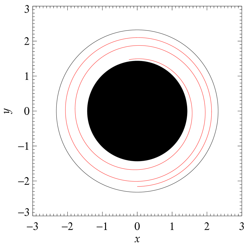
As mentioned above, time-dependent spectra are expected to eliminate a great deal of uncertainty in studying accretion disks (e.g. Done & Gierliński 2003). As an example of using ky outside of xspec, Fig. 1 represents an evolving spectral line in a dynamical diagram: a localized spot, free-falling from the marginally stable orbit down towards the black-hole horizon. Intrinsic emissivity is assumed to fade gradually with the distance from the spot centre, with characteristic diameter of the spot $\sim 0.4GM/c^{2}$ ($\beta=100$ in kyspot), but it is kept constant in time. Therefore the figure reflects the effect of changing energy shift along the spot trajectory. The in-spiral motion starts just below the marginally stable orbit and it proceeds down to the horizon, maintaining the specific energy and angular momentum of its initial circular orbit. One can easily recognise that variations in redshift could hardly be recovered from data if only time-averaged spectrum were available. In particular, the motion above $r_{\rm{}ms}(a)$ near a rapidly spinning black hole is difficult to distinguish from a descent below $r_{\rm{}ms}(0)$ in the non-rotating case.

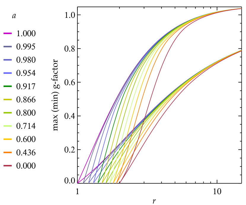
Before time-resolved spectra are available with sufficient quality, preliminary considerations can be based on the extremal values, and the range, of energy shift, $g_{+}$ and $g_{-}$, as well as the relative time delay which photons experience when arriving at the observer’s location from different parts of the disk. This is particularly relevant for some narrow lines whose redshift can be determined more accurately than if the line is broad (e.g. Turner et al. 2002; Guainazzi 2003; Yaqoob et al. 2003). Careful discussion of $g_{\pm}$ can, in principle, circumvent the uncertainties which are introduced by uncertain form of the intrinsic emissivity of the disk and yet still constrain some of parameters. Advantages of this technique were pointed out already by Cunningham (1975) and it was further developed by Pariev, Bromley & Miller (2001).

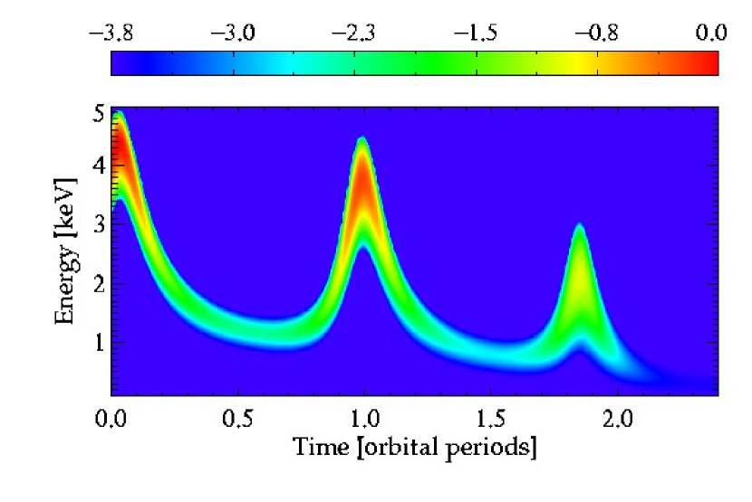
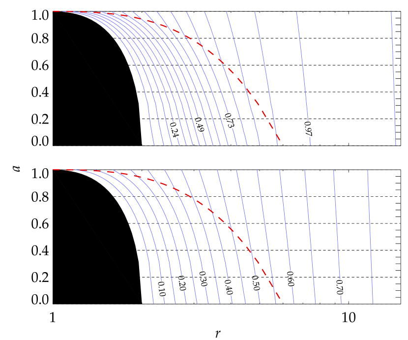
Fig. 2 shows the extremal values of the redshift factor for $\theta_{\rm{}o}=30^{\circ}$ (which often seems to be preferred by the observational data). These were computed along $r=\mbox{constant}$ circles in the disk plane, together with the corresponding contour lines of $g_{\pm}=\mbox{constant}$ in the plane $a$ versus $r$. In other words, radiation is supposed to originate from radius $r$ in the disk, but it experiences a different redshift depending on the polar angle. Contours of the redshift factor provide a very useful and straightforward technique to determine the position of a flare or a spot, provided that a narrow spectral line is produced and measured with sufficient accuracy. The most direct use of extremal $g$-values would be, if one were able to measure variations of the line profile from its lowest-energy excursion (for $g_{-}$) and highest-energy excursion (for $g_{+}$), i.e. over a complete cycle. Even partial information can help to constrain models (for example, the count rate is expected to dominate the observed line at the time that $g=g_{+}$, and so the high-energy peak is easier to detect). While it is very difficult to achieve sufficient precision on the highly shifted and damped red wing of a broad line, prospects for using narrow lines is indeed interesting, provided that they originate close enough to the black hole and that sufficient resolution is achieved both in the energy and time domains.

Fig. 2 also makes it clear that it is possible in principle (but intricate in practice) to deduce the $a$-parameter value from spectra. It can be seen from the redshift factor that the dependence on $a$ is rather small and it quickly becomes negligible if the light from the source is dominated by contributions from $r\gtrsim 10$. For example, setting $r=7$ and $\theta_{\rm{}o}=30^{\circ}$, one finds that the relative difference between $g_{+}(a=1)$ and $g_{+}(a=0)$ amounts to only $\sim 2\%$. A similar value comes out for $g_{-}$, and this also roughly corresponds to the precision which is needed in order to be able to reveal the effect of black hole rotation. Notice, however, that this is in principle achievable by the Chandra gratings and the Astro–E2 calorimeter. It may also be achievable by XMM–Newton with high signal-to-noise data, and of course the effect would be more pronounced in case of a source seen edge-on.

Other user-defined emissivities can be easily adopted. This can be achieved either by using the convolution component kyconv or by adding a new user-defined model to xspec. The latter method is more flexible and faster, and hence recommended. In both approaches, the ray-tracing routine is linked and used for relativistic blurring. Naturally, by adding new emissivity laws one invariably introduces additional freedom (for example, the height $h$ of the primary source in the lamp-post model). It is worth repeating that caution is always necessary because the predictive power of the model rapidly decays with the number of parameters.

We conclude this section by summarizing the way of using the new model: Time-dependent spectra are computed by specifying the photon numbers emitted from the disk, $N_{\rm{}loc}(E,r,\varphi,\mu_{\rm{}loc},t)$, where $r$ and $\varphi$ are polar coordinates in the disk plane, $\mu_{\rm{}loc}$ is cosine of the emission angle with respect to the disk normal, $t$ is Boyer-Lindquist time in the Kerr metric, and $N$ comes out in $\mbox{photons}\,\mbox{cm}^{-2}\,\mbox{s}^{-1}\,\mbox{sr}^{-1}\,\mbox{keV}^{-1}$. Naturally, mean spectra represent a special case in which time dependence of the source emissivity is not considered.

3 Application to MCG–6-30-15

The Seyfert 1 galaxy MCG–6-30-15 is a unique source in which the evidence of a broad and skewed Fe K$\alpha$ line has led to a wide acceptance of models with an accreting black hole in the nucleus (Tanaka et al. 1995; Iwasawa et al. 1996; Nandra et al. 1997; Guainazzi et al. 1999; Fabian & Vaughan 2003). Being a nearby AGN (the galaxy redshift is $z=0.0078$), this source offers an unprecedented opportunity to explore directly the pattern of the accretion flow onto the central hole. The Fe K line shape and photon redshifts indicate that a large fraction of the emission originates from $r\lesssim 10$ ($GM/c^{2}$). The mean line profile derived from XMM–Newton observations is similar to the one observed previously using ASCA. The X-ray continuum shape in the hard spectral band was well determined from BeppoSAX data (e.g. Guainazzi et al. 1999).

Table 3: Spectral fitting results for MCG–6-30-15 using the ky model.

#	$a$	$\theta_{\rm{}o}$	Continuum			Broad Fe K$\alpha$ line							$\chi^{2}$
			$\Gamma_{\rm{}c}$	$\alpha_{\rm{}c}$		$r_{\rm{}in}\!-r_{\rm{}h}$	$r_{\rm{}b}\!-r_{\rm{}h}$	$r_{\rm{}out}\!-r_{\rm{}h}$	$\alpha_{\rm{}in}$	$\alpha_{\rm{}out}$	EW		(dof)
1	$0.35^{+0.57}_{-0.30}$	$31.8\pm 0.3$	$2.01\pm 0.02$	$1.0^{+9}_{-1}$		$5.1\pm 0.2$	–	$11.4\pm 0.8$	–	$3.9\pm 0.6$	$258^{+26}_{-13}$		$\frac{368.8}{(329)}$
2a	$0.99\pm 0.01$	$40.4\pm 0.6$	$2.03\pm 0.02$	$5.5^{+6}_{-2}$		$0.67\pm 0.04$	$3.35\pm 0.05$	$40^{+960}_{-33}$	$6.9^{+0.5}_{-0.4}$	$9.7^{+0.3}_{-0.8}$	$268\pm 13$		$\frac{308.6}{(330)}$
2b	$0.72^{+0.12}_{-0.30}$	$28.5\pm 0.5$	$2.01\pm 0.01$	$0.1^{+2}_{-0.1}$		$0.65\pm 0.35$	$2.1\pm 0.2^{\,{\dagger}}$ $7.2\pm 0.2$	$48^{+200}_{-25}$	$8.1^{+1.4}_{-0.9}$	$4.9^{+0.4}_{-0.3}$	$241^{+13}_{-10}$		$\frac{313.5}{(330)}$
2c	$0.25\pm 0.03$	$27.6\pm 0.6$	$1.97\pm 0.02$	$3.1^{+0.3}_{-0.1}$		$1.23\pm 0.06$	$4\pm 0.02$	$109^{+20}_{-10}$	$9.2\pm 0.2$	$3.1\pm 0.1$	$267\pm 10$		$\frac{313.9}{(330)}$

Best-fitting values of the important parameters and their statistical errors for models #1–2, described in the text. The models include broad Fe K$\alpha$ and Fe K$\beta$ emission lines, a narrow Gaussian line at $\sim 6.9$ keV, and a Compton-reflection continuum from a relativistic disk. These models illustrate different assumptions about intrinsic emissivity of the disk (the radial emissivity law need not to be a simple power law, but axial symmetry has been still imposed here). The inclination angle $\theta_{\rm{}o}$ is in degrees, relative to the rotation axis; radii are expressed as an offset from the horizon (in $GM/c^{2}$); the equivalent width, EW, is in electron volts.
^† Two values of the transition radius define the interval $\langle{}r_{\rm{}b-},r_{\rm{}b+}\rangle$ where reflection is diminished.

Figure 3: Confidence contours around the best-fitting parameter values (indicated by a cross). Left: the case of a single line-emitting region (model #1 with zero emissivity for $r<r_{\rm{}ms}$). Right: the case of a non-monotonic radial emissivity, model #2b. The joint two-parameter contour levels for $a$ versus $\theta_{\rm{}o}$ correspond to 68%, 95% and 99% confidence.

To illustrate the new ky model capabilities, we used our code to analyze the mean EPIC PN spectrum which we compiled from the long XMM–Newton 2001 campaign (e.g., as described in Fabian et al. 2002). The data were cleaned and reduced using standard data reduction routines, employing SAS version 5.4.1. We summed the EPIC PN data from five observations made in the interval 11 July 2001 to 04 August 2001, obtaining a total good exposure time of $\sim 290$ ks (see Fabian et al. 2002 for details of the observations). The energy range was restricted to $3$–$10$ keV with $339$ energy bins, unless otherwise stated, and models were fitted by minimizing the $\chi^{2}$ statistic. Statistical errors quoted correspond to $90$% confidence for one interesting parameter (i.e. $\Delta\chi^{2}=2.706$), unless otherwise stated.

No absorber was taken into account; the assumption here is that any curvature in the spectrum above 3 keV is not due to absorption, and only due to the Fe K line. We remind the reader that the Fe K emission line dominates around the energy $6$–$7$ keV, but it has been supposed to stretch down to $\sim 3$ keV or even further. We emphasize that our aim here is to test the hypothesis that if all of the curvature is entirely due to the broad Fe K feature, is it possible to constrain $a$ of the black hole? Obviously, if the answer to this is ‘no’, it will also be negative if some of the spectral curvature between $\sim 3$–$5$ keV is due to processes other than the Fe K line emission.

We considered Fe K$\alpha$ and Fe K$\beta$ iron lines (with their rest-frame energy fixed at $E_{\rm{}loc}=6.400$ and $7.056$ keV, respectively), a narrow-line feature (observed at $E_{\rm{}obs}\sim 6.9$ keV) modeled as a Gaussian with center energy, width, and intensity free, plus a power-law continuum. We used a superposition of two kygline models to account for the broad relativistic K$\alpha$ and K$\beta$ lines, zgauss for the narrow, high-energy line (which we find to be centered at $6.86$ keV in the source frame, slightly redshifted relative to $6.966$ keV, the rest-energy of Fe Ly$\alpha$), and kyhrefl for the Comptonized continuum convolved with the relativistic kernel. We assumed that the high-energy narrow line is non-relativistic. Note that an alternative interpretation of the data (as pointed out by Fabian et al. 2002) is that there is not an emission line at $\sim 6.9$ keV, but He-like resonance absorption at $\sim 6.7$ keV. This would not affect our conclusions. The ratio of the intensities of the two relativistic lines was fixed at $I_{\rm{K\beta}}/I_{\rm{K\alpha}}=0.1133$ ($=17/150$), and the iron abundance for the Compton-reflection continuum was assumed to be three times the solar value (Fabian et al. 2002). We used the angles $\theta_{\rm{}min}=0^{\circ}$ and $\theta_{\rm{}max}=90^{\circ}$ for local illumination in kyhrefl (these values are equivalent to central illumination of an infinite disk). The normalization of the Compton-reflection continuum relative to the direct continuum is controlled by the effective reflection ‘covering factor’, $R_{\rm{}c}$, which is the ratio of the actual reflection normalization to that expected from the illumination of an infinite disk (see Appendix). Also $r_{\rm{}out}$ (outer radius of the disk), $\alpha_{\rm{}c}$ (slope of power-law continuum radial emissivity in the kyhrefl model component), as well as $R_{\rm{}c}$, were included among the free parameters, but we found them to be only very poorly constrained. Weak constraints on $\alpha_{\rm{}c}$ and $R_{\rm{}c}$ are actually expected in this model for two reasons. Firstly, in these data the continuum is indeed rather featureless. Secondly, the model continuum was blurred with the relativistic kernel of kyhrefl, and so the dependence of the final spectrum on the exact form of emissivity distribution over the disk must be quite weak.

Model #1. Using a model with a plain power-law radial emissivity on the disk, we obtained the best-fitting values for the following set of parameters: $a$ of the black hole, disk inclination angle $\theta_{\rm{}o}$, radii of the line-emitting region, $r_{\rm{}in}<r<r_{\rm{}out}$, the corresponding radial emissivity power-law index $\alpha$ of the line emission, as well as the radial extent of the continuum-emitting region, its photon index $\Gamma_{\rm{}c}$, and the corresponding $\alpha_{\rm{}c}$ for the continuum. Notice that $\Gamma_{\rm{}c}$ and $\alpha_{\rm{}c}$ refer to the continuum component before the relativistic kernel was applied to deduce the observed spectrum. As a result of the integration across the disk, the model weakly constrains these parameters.

There are two ways to interpret this. A model which is over-parameterized is undesirable from the point of view of deriving unique model parameters from modeling the data. However, another interpretation is that a model with a greater number of parameters may more faithfully reflect the real physics and it is the actual physical situation which leads to degeneracy in the model parameters. The latter implies that some model parameters can never be constrained uniquely, regardless of the quality of the data. In practice one must apply both interpretations and assess the approach case by case, taking into account the quality of the data, and which parameters can be constrained by the data and which cannot. If preliminary fitting shows that large changes in a parameter do not affect the fit, then that parameter can be fixed at some value obtained by invoking physically reasonable arguments pertaining to the situation.

We performed various fits with the inner edge tied to the marginally stable orbit and also fits where $r_{\rm{}in}$ was allowed to vary independently. Free-fall motion with constant angular momentum was assumed below $r_{\rm{}ms}$, if the emitting region extended that far. Table 3 gives best-fitting values of the key relativistic line and continuum model parameters for the case in which $r_{\rm{}in}$ and $a$ were independent.

Next, we froze some of the parameters at their best-fit values and examined the $\chi^{2}$ space by varying the remaining free parameters. That way we constructed joint confidence contours in the plane $a$ versus $\theta_{\rm{}o}$ (see left panel of Fig. 3). These representative plots demonstrate that $\theta_{\rm{}o}$ appears to be tightly constrained, while $a$ is allowed to vary over a large interval around the best fit, extending down to $a=0$.

Model #2. We explored the possibility that the broad-line emission does not conform to a unique power-law radial emissivity but that, instead, the line is produced in two concentric rings (a ‘dual-ring’ model). This case can be considered as a toy model for a more complex (non-power law) radial dependence of the line emission than the standard monotonic decline, which we represent here by allowing for different values of $\alpha$ in the inner and outer rings: $\alpha_{\rm{}in}$ and $\alpha_{\rm{}out}$. Effectively, large values of the power law index represent two separate rings. The two regions are matched at the transition radius, $r=r_{\rm{}b}$, and so this is essentially a broken power law. We explored both the case of continuous and discontinuous line emissivity at $r=r_{\rm{}b}$. Notice that the double power-law emissivity arises naturally in the lamp-post model (Martocchia et al. 2000) in which the disk irradiation and the resulting Fe K$\alpha$ reflection are substantially anisotropic due to fast orbital motion in the inner ring. Although the lamp-post model is very simplified in several respects, namely the way in which the primary source is set up on the rotation axis, one can expect fairly similar irradiation to arise from more sophisticated schemes of coronal flares distributed above the disk plane. Also, in order to provide a physical picture of the steep emissivity found in XMM–Newton data of MCG–6-30-15, Wilms et al. (2001) invoked strong magnetic stresses acting in the innermost part of the system, assuming that they are able to dissipate a considerable amount of energy in the disk at very small radii. Intense self-irradiation of the inner disk may further contribute to the effect.

This more complex model is consistent with the findings of Fabian et al. (2002). Indeed, the fit is improved relative to models with a simple emissivity law because the enormous red wing and relatively sharp core of the line are better reproduced thanks to the contribution from a highly redshifted inner disk (see Table 3, model #2a). For the same reason that the more complex model reproduces the line core along with the red wing well, the model prefers higher values of $a$ and $\theta_{\rm{}o}$ than what we found for the case #1. Notice that $a\rightarrow 1$ implies that all radiation is produced above $r_{\rm{}ms}$. Maximum rotation is favoured with both $a$ and $\theta_{\rm{}o}$ appearing to be tightly constrained near their best-fit values. Likewise for the continuum radial emissivity indices. There is a certain freedom in the parameter values that can be accomodated by this model. By scanning the remaining parameters, we checked that the reduced $\chi^{2}\sim 1$ can be achieved also for $a$ going down to $\sim 0.9$ and $\theta_{\rm{}o}\sim 37^{\circ}$. This conclusion is also consistent with the case for large $a$ in Dabrowski et al. (1997); however we actually do not support the claim that the current data require a large value of $a$. As shown below, reasonable assumptions about intrinsic emissivity can fit the data with small $a$ equally well.

In model #2a, small residuals remain near $E\sim 4.8$ keV (at about the $\sim 1$% level), the origin of which cannot easily be clarified with the time-averaged data that we employ now. The excess is reminiscent of a Doppler horn typical of relativistic line emission from a disk, so it may also be due to Fe K$\alpha$ emission which is locally enhanced on some part of the disk. We were able to reproduce the peak by modifying the emissivity at the transition radius, where the broken power-law emissivity changes its slope (model #2b). We can even allow non-zero emissivity below $r_{\rm{}ms}$ (the inner ring) with a gap of zero emissivity between the outer edge of the inner ring and the inner edge of the outer one. The inner ring, $r_{\rm{}in}{\leq}r{\leq}r_{\rm{}b-}$, contributes to the red tail of the line while the outer ring, $r_{\rm{}b+}{\leq}r{\leq}r_{\rm{}out}$, forms the main body of the broad line. The resulting plot of joint confidence contours of $\theta_{\rm{}o}$ versus $a$ is shown in Fig. 3 (right panel) In order to construct the confidence contours we scanned a broad interval of parameters, $0<a<1$ and $0<\theta_{\rm{}o}<45^{\circ}$; here, detail is shown only around the minimum $\chi^{2}$ region.

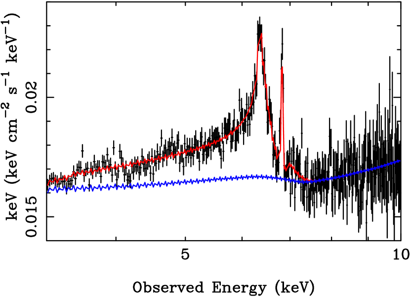
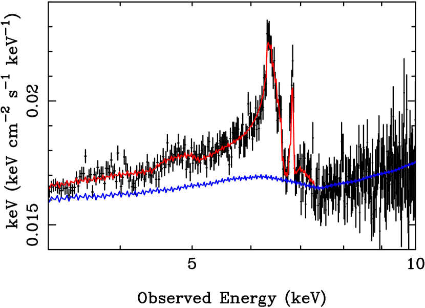
Two examples of the spectral profiles are shown in Fig. 4. It can be seen that the overall shapes are very similar and the changes concern mainly the red wing of the profile. For completeness we also fitted several modifications of the model #2 and found that with this type of disk emissivity (i.e. one which does not decrease monotonically with radius) we can still achieve comparably good fits which have small values of $a$. The case #2c in Table 3 gives another example. This shows that one cannot draw firm conclusions about $a$ (and some of the other model parameters) based on the redshifted part of the line using current data. The data used here represent the highest signal-to-noise relativistically broadened Fe K line profile yet available for any AGN.

The differences in $\chi^{2}$ between model #1 and models #2a, 2b, and 2c are very large ($\sim 60$) for only one additional free parameter, so all variations of model 2 shown are better fits than the case #1. We note that formally, model #2a and #2c appear to constrain $a$ much more tightly than model #1. The issue here is that the values of $a$ can be completely different, with the statistical errors on $a$ not overlapping (compare, for example, model #2a and #2c in Table 3). This demonstrates that, at least for the parameter $a$, it is not simply the statistical error only which determines whether a small $a$ value is or is not allowed by the data. We confirmed this conclusion with more complicated models obtained in ky by relaxing the assumption of axial symmetry; additional degrees of freedom do not change the previous results.

One should bear in mind a well-known technical difficulty which is frequently encountered while scanning the parameter space of complex models and producing confidence contour plots similar to Fig. 3. That is, in a rich parameter space the procedure may be caught in a local minimum which produces an acceptable statistical measure of the goodness of fit and appears to tightly constrain parameters near the best-fitting values. However, manual searching revealed equally acceptable results in rather remote parts of the parameter space. Indeed, as the results above show, we were able to find acceptable fits with the central black hole rotating either slowly or rapidly (in terms of the $a$ parameter). This fact is not in contradiction with previous results (e.g. Fabian et al. 2002) because we assumed a different radial profile of intrinsic emissivity, but it indicates intricacy of unambiguous determination of model parameters. We therefore need more observational constraints on realistic physical mechanisms to be able to fit complicated models to actual data with sufficient confidence (Ballantyne, Ross & Fabian 2001; Nayakshin & Kazanas 2002; Różańska et al. 2002).

Figure 4: Spectrum and best-fitting model for the XMM–Newton data for MCG–6-30-15 in which the Fe K line originates in a dual-ring. The models 2a (left) and 2b (right) are shown in comparison. See Table 3 for the model parameters. The continuum component (kyhrefl) is also plotted. The data points are not unfolded: the spectrum in these units was made by multiplying the ratio of measured counts to the counts predicted by the best-fitting model and then this ratio was multiplied by the best-fitting model and then by $E^{2}$.

We have seen that the models described above are able to constrain parameters with rather different degrees of uncertainty. It turns out that the more complex type #2 models (i.e. those that have radial emissivity profiles which are non-monotonic or even have an appreciable contribution from $r<r_{\rm{}ms}$) provide better fits to the data but a physical interpretation is not obvious. Ballantyne, Vaughan & Fabian (2003) also deduce a dual-reflector model from the same data and propose that the outer reflection is due to the disk being warped or flared with increasing radius.

4 Discussion and Conclusions

We have presented an extended computational scheme which can be conveniently employed to examine predicted X-ray spectral features from black-hole accretion disks. As mentioned above, a one-dimensional version of the code basically reproduces previous methods, with the addition of the option to vary more parameters (e.g. $a$). The current two-dimensional version also accomodates non-axisymmetric and time-evolving emissivity from a geometrically thin disk. The new tool facilitates accurate comparisons between model spectra and actual data. It provides also polarimetric information. One can even substitute other tables for the Kerr metric tables to explore different specetime. However, we defer detailed discussion of these latter capabilities to a future paper. Furthermore, work is in progress to include realistic emissivities relevant to different physical situations, in order to allow for the intrinsically three-dimensional geometry of the sources (e.g. an optically-thin corona above the disk), and to parallelize the code.

Recently, several research groups have embarked on projects to compare theoretical predictions of intrinsic emissivity of accretion disks with observational data obtained by X-ray satellites. This approach offers a fascinating opportunity to explore processes near black-hole sources, both AGNs and BHCs, and to estimate physical parameters of black holes themselves. In order to limit the number of unknown model parameters and to alleviate the computational burden of the fit procedure, simplifications on the model emissivity (for example, stationarity and/or axial symmetry) have been often imposed. Naturally, fitting data with complex models is computationally more demanding.

To summarize, we have illustrated the code by following common practice and employing minimisation of $\chi^{2}$ to find the best-fitting parameter values for the highest signal-to-noise Fe K line profile available to date—from the XMM–Newton campaign of the Seyfert 1 galaxy MCG–6-30-15. The new model can vary more of the parameters than previous variants of the disk-line scheme allowed, which seems to be necessary in view of the fact that simple prescriptions for intrinsic emisivity (axisymmetric, radially monotonic, etc.) are not adequate to reflect realistic simulations of accretion flows. It is without much surprise that a complex model exhibits an intricate $\chi^{2}$ space in which ambiguities arise with multiple islands of acceptable parameters. The mean XMM–Newton spectrum of MCG–6-30-15 analyzed here justifies rejection of the often-used plain power-law emissivity that depends solely on radius from the black hole. However, we cannot arbitrate the issue of non-monotonic emissivity versus a non-axisymmetric one. Due to the inherent degeneracy in time-averaged spectra, both alternatives can reproduce these data with reasonable parameters. In other words, $a$ of the black hole cannot be unambiguously determined if complex (realistic) emissivities are adopted.

It is clear that the relativistic line profiles affected by strong gravity are such that it is very difficult to recover unambiguous information about the key parameters, such as black-hole spin, disk inclination angle, and inner disk radius. This is because even with increased throughput, energy resolution and signal-to-noise, the smooth, featureless tails of the time-averaged line profiles do not retain sufficient information to break the degeneracies between the dependences on the black-hole, accretion disk, and line emissivity parameters.

Higly specific spectral shapes could actually be provided by contributions to the line profile from higher-order images, whose form inherits unique information about space-time of the black hole. It may appear rather unlikely that higher-order images could be discovered in spectra of AGNs, because this would require to see an unobscured inner disk at large (almost edge-on) inclination.

As the data improve, the important measurable quantities that will constrain parameters when compared with the models are: (i) the slope of the red wing, (ii) the energy of the cut-off of the blue side of the line profile, and (iii) the detailed shape of the blue peak (see Figs. 7–9 and further discussion in the Appendix). The extreme part of the red wing will not be as useful because it will always be difficult to tell where the line emission joins the continuum no matter how good the data are, and also because there is often no prominent sharp feature in the red wing since the red Doppler peak is too smeared out when the line emission extends too close to the black hole. In addition, time variability will be extremely important. No matter how, or if, the line emission responds to the continuum, we know that the disk inclination and black-hole spin very likely do not change during different snapshots. Therefore any differences in the snapshot line profiles must be due only to changes in the line emissivity, in terms of its radial and azimuthal distribution and/or its radial extent ($r_{\rm{}in}$ and $r_{\rm{}out}$). Combining these approaches and collecting enough snapshots may provide sufficient information to uniquely determine one of the parameters, such as black-hole spin.

Appendix A The Numerical Code: Tests and Examples

Figure 5: Graphical representation of the contents of the data tables for the ky model used in the computations. Several sets of contour plots capture the equatorial plane with an increasing resolution near the black-hole horizon. Here we show the effect of energy shift $g{\equiv}g(r,\varphi)$. Lengths are in $GM/c^{2}$ (radius up to $r=10^{3}$ in the coarsest grid). Values are encoded by a colour scale, as indicated in each graph. Key parameters are: $\theta_{\rm{}o}=30^{\circ}$, and $a=0.9987$ (corresponding to $r_{\rm{}h}\dot{=}1.05$, $r_{\rm{}ms}\dot{=}1.2$). Clock-wise distortion of the contours is due to frame-dragging near a rapidly rotating Kerr black hole, and it is clearly visible in Boyer-Lindquist coordinates here. High accuracy of the tables has been achieved by eliminating this influence, with the aid of an appropriate transformation. In the upper left panel, corresponding to the region closest to the black hole, the horizon has been brought to the origin by the transformation of coordinates described in the text.

Figure 6: The same as in previous figure, but now showing the gravitational lensing effect in the disk. Contours correspond to lines of constant magnification. They were computed by solving geodesic deviation equations in the Kerr metric.

Figure 7: Comparative examples of simple line profiles, showing a theoretical line ($E_{\rm{}loc}=6.4\,$keV) with relativistic effects originating from a black-hole accretion disk. Different sizes of the annular region (axially symmetric) have been considered, assuming that the intrinsic emissivity obeys a power law in the radial direction ($\alpha=3$). Resolution of the line-emitting region was $n_{r}{\times}n_{\varphi}=3000\times 1500$ with a non-equidistant layout of the grid in Kerr ingoing coordinates, as described in the text. Left: dependence on the inner edge. Values of $r_{\rm{}in}$ are indicated in the plot (the outer edge has been fixed at the maximum radius covered by our tables, $r_{\rm{}out}=10^{3}$). Right: dependence on $r_{\rm{}out}$ (with the inner edge at horizon, $r_{\rm{}in}=r_{\rm{}h}$). Other key parameters are: $\theta_{\rm{}o}=45^{\circ}$, $a=1.0$. Locally isotropic emission was assumed in the disk co-rotating frame.

Figure 8: More calculated line profiles, as in the previous figure. Left: Line profiles for different values of $\alpha$. Notice the enhanced red tail of the line when the intrinsic emission is concentrated to the center of the disk. Right: Line emission originating from four different azimuthal segments of the disk. This plot can serve as a toy model of non-axisymmetric emissivity or to illustrate the expected effects of disk obscuration. Obviously, the receding segment of the disk contributes mainly to the low-energy tail of the line while the approaching segment constitutes the prominent high-energy peak. These two plots illustrate a mutual interplay between the effect of changing $\alpha$ and the impact of obscuration, which complicates interpretation of time-averaged spectra. The radial range is $r_{\rm{}h}<r<10^{3}$ in both panels.

Figure 9: Dependence on observer inclination (values of $\theta_{\rm{}o}$ are given in the plot). Left: non-rotating black hole, $a=0$. Right: maximally rotating black hole, $a=1$. Other parameters as in Fig. 7.

Geometrical optics is adequate to formulate the ray tracing problem in rigorous manner (Schneider, Ehlers & Falco 1992). Physically, one has to consider a ray bundle connecting the source and the observer. We realize that the photon number is conserved in a bundle along the photon ray. Furthermore, this number is observer-independent quantity. Four-momentum of each photon is parallely transported along the ray. On a practical side, to achieve fast computations of observed spectra and for data fitting we produced accurate tables describing the Kerr metric, ray-tracing equations and the equations of geodesic deviation. These were solved in well-behaved coordinates. This choice allows one to map the whole region, from the outer edge of the disk down to the black hole horizon, where dragging effects are prominent. Also, caustics can play a role for large inclination (Rauch & Blandford 1994). When integration of light rays is accomplished, we transform results back to Boyer-Lindquist coordinates, so that the intrinsic emissivity of the disc can be conveniently defined as a function of $r$, $\varphi$ and $t$ in the disk plane. Here we briefly summarise the adopted approach.

The source appears as a point-like object for a distant observer, so that the observer actually measures the flux entering the solid angle ${\rm d}\Omega_{\rm obs}$, which is associated with the detector area ${\rm d}S_{\rm obs}{\equiv}D^{2}\,{\rm d}\Omega_{\rm obs}$ (this relation defines the distance $D$). We denote total photon flux received by a detector,

$$N^{S}_{\rm{}obs}(E)\equiv\frac{{\rm d}n(E)}{{\rm d}t\,{\rm d}S_{\rm obs}}={\int}N_{\rm loc}(E/g)\,g^{2}\,{\rm d}\Omega,$$ (A1)

where

$$N_{\rm loc}(E_{\rm loc})\equiv\frac{{\rm d}n_{\rm loc}(E_{\rm loc})}{{\rm d}\tau\,{\rm d}S_{\rm loc}\,{\rm d}\Omega_{\rm loc}}$$ (A2)

is local photon flux at the disk, ${\rm d}n(E)$ is the number of photons with energy in interval ${\langle}E,E+{\rm d}E\rangle$ and $g=E/E_{\rm{}loc}$ is the redshift factor. Note that $N_{\rm{}loc}(E_{\rm{}loc})$ may vary over the disk, change in time, and it can also depend on the emission angle (for the sake of brevity of formulae, we do not always write this dependence explicitly).

The emission arriving in solid angle ${{\rm d}\Omega}$ originates from area ${\rm d}S_{\rm loc}$ on the disk. Hence, in our computations we want to integrate the flux contributions over a fine mesh on the disk surface. To this aim, we adjust eq. (A1) to the form

$$N^{S}_{\rm{}obs}(E)\equiv\frac{1}{D^{2}}{\int}N_{\rm loc}(E/g)\,g^{2}\,\frac{D^{2}\,{\rm d}\Omega}{{\rm d}S_{\rm loc}}\,{\rm d}S_{\rm loc}=\frac{1}{D^{2}}{\int}N_{\rm{}loc}(E/g)\,g^{2}\,\frac{{\rm d}S_{\rm f}}{{\rm d}S_{\rm loc}}\,\frac{{\rm{}d}S_{\rm loc}}{{\rm d}S}\,{\rm d}S\,.$$ (A3)

Here ${{\rm{}d}S_{\rm f}}$ denotes an element of area on the disk perpendicular to light rays (corresponding to the solid angle ${\rm d}\Omega$ in flat space-time), and ${\rm d}S\equiv r\,{\rm d}r\,{\rm d}\varphi$ stands for area in Boyer-Lindquist coordinates lying in the disk plane from which photons are emitted. The integrated flux per unit solid angle is

$${\rm d}N^{\Omega}_{\rm obs}(E,t) \equiv N^{\Omega}_{\rm obs}(E,t)\,{\rm d}E$$ (A4)

$$= N_{0}\int_{r_{\rm in}}^{r_{\rm out}}\!\!{\rm d}r\int_{\varphi_{\rm{}min}}^{\varphi_{\rm{}max}}\!\!{\rm d}\varphi\int_{E/g}^{(E+{\rm d}E)/g}\!\!{\rm d}E_{\rm loc}\,N_{\rm loc}(E_{\rm loc},r,\varphi,\mu_{\rm loc},t_{0})\,g^{2}\,l\,r,$$

where $t_{0}\,\equiv\,t-\Delta t$ is time coordinate corrected for the light-time effect,

$$l=\frac{{\rm d}S_{\rm f}}{{\rm{}d}S_{\rm loc}}=\frac{{\rm d}S_{\rm f}}{{\rm d}S_{\perp}}\mu_{\rm loc}$$ (A5)

is the lensing factor in the limit $D\rightarrow\infty$ (keeping $D^{2}\,{\rm d}\Omega$ constant), $\mu_{\rm loc}$ is the cosine of the local emission angle, ${\rm d}S_{\perp}$ is proper area at the disk perpendicular to light rays and corresponding to ${\rm d}\Omega$. In eq. (A4) we used transformation of the proper area element, ${{\rm d}S_{\rm loc}}$,

$$\frac{{\rm d}S_{\rm loc}}{{\rm d}S}=g^{-1}.$$ (A6)

Finally, $N^{\Omega}_{\rm obs}(E,t)$ is the output of the model computations.

In eq. (A4),$N_{0}$ is a normalization constant of the model. For line emission, normalization is chosen in such a way that the total flux from the disk is unity. In the case of a continuum model, the flux is normalized to unity at certain value of observed energy (typically at $E=1$ keV, as in other xspec models). Notice that default normalization has been changed in Figs. 7–9 for the sake of clarity.

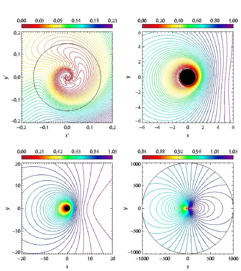
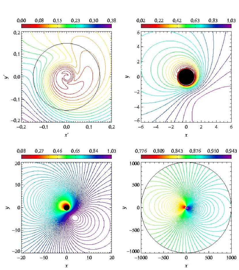
We employed the Bulirsch-Stoer method for numerical integration. Four sets of data tables were pre-computed and stored with the necessary information about photons received from different regions of the source. Specifically, separate tables hold information on (i) the energy shift ($g$-factor, or the ratio of energy of a photon received by an observer at infinity to the intrinsic energy when emitted at the disk), (ii) the lensing effect (the ratio $l$ of the area subtended by photons at infinity, perpendicular to light rays through which photons arrive at the detector, to the area on the disk from where these photons originate), (iii) the mutual delay of the photons arriving at the observer’s location (i.e. relative time lags $\Delta{t}$), and (iv) the local emission direction $\mu_{\rm{}loc}$ with respect to the disk normal (evaluated in the disk co-rotating frame).

The problem of directional distribution of the reflected radiation is quite complicated and the matter has not been completely settled yet (e.g. George & Fabian 1991; Ghisellini, Haardt & Matt 1994; Życki & Czerny 1994; Magdziarz & Zdiarski 1995). A specific angular dependence is often assumed in models, such as the limb-darkening in laor xspec model, $I(\mu_{\rm loc})\,\propto\,1+2.06\mu_{\rm loc}$. However, it has been argued that limb-brightening may actually occur in the case of strong primary irradiation of the disk, and this is relevant for accretion disks near black holes where the effects of emission anisotropy are crucial (Czerny et al. 2004). We find that the spectrum of the inner disk turns out to be very sensitive to the adopted angular dependence of the emission, and so the possibility to modify this profile and examine the results using ky appears to be rather useful (we set locally isotropic emission as default). Impact of the darkening law on the reflection spectrum is connected with the assumed rotation law of the disk material. As mentioned above, we assumed Keplerian circular motion for $r{\geq}r_{\rm{}ms}$. For $r<r_{\rm{}ms}$ we assumed free-fall trajectories, maintaining constant orbital energy and angular momentum.

All data tables are stored in fits format and loaded in memory only once, when the routine is initiated. Examples of the contents of the data tables, illustrating the effects of frame-dragging, are shown in Figures 5–6 for given choices of $a$ and $\theta_{\rm{}o}$. The graphs represent a top view of the equatorial plane, each one on four different spatial scales. In practice we have chosen $r_{\rm{}out}=10^{3}$ (Boyer-Lindquist radius) as a maximum outer limit of the disk, but the most dramatic dependences on, for example $a$, happen much closer to the horizon. In the upper left panels of Figs. 5 and 6 we define the radial coordinate in a different way to that in the other panels. Specifically, we use ${r^{\prime}}^{2}\equiv{x^{\prime}}^{2}+{y^{\prime}}^{2}=(r-r_{\rm h})^{2}$. The use of $r^{\prime}$ brings the horizon to the origin so that the region just outside it is well resolved in the plots that show the region closest to the black hole. In these graphs, the observer is located at the top of the pictures with an inclination angle of $30^{\circ}$ relative to the rotation axis. The marginally stable orbit is also shown (drawn as a circle) where relevant.

Despite the fact that the particular choice of the graphical representation is a technicality to certain extent, we find these kinds of graphs useful for quick estimations of the expected range of energy shifts, fluctuations of radiation flux, time delay effects etc. For example, we notice that with the adopted (typical) value of $\theta_{\rm{}o}=30^{\circ}$, the lensing cannot account for more than a few percent effect on observed count rates. Lensing, however, becomes important for edge-on orientation of the disk, as can be seen from the tables with larger values of $\theta_{\rm{}o}$. We therefore arranged a systematic atlas of the tables for different values of angular momentum and observer inclination. Further, we produced their transformation from Boyer-Lindquist $(r,\varphi,t)$ to Kerr ingoing coordinates (in which the effect of frame dragging is largely eliminated), and the same for other relevant quantities (time delay and the emission angle in the disk). It is worth noticing that different space-time metric and the disk rotation law can be accomodated simply by replacing the data tables. Also, transfer of Stokes parameters can be computed, and to this aim we computed data tables which are needed for polarimetry in strong gravity. However, this discussion remains beyond the scope of the present paper.

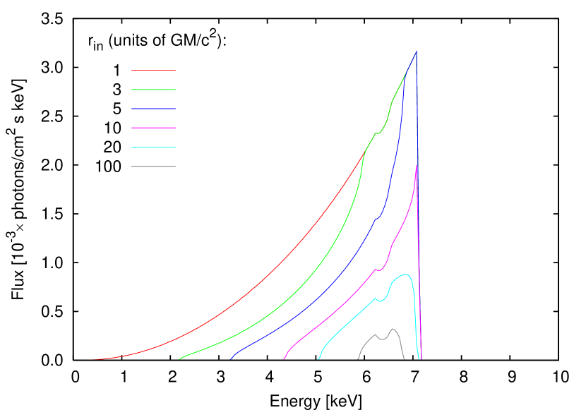
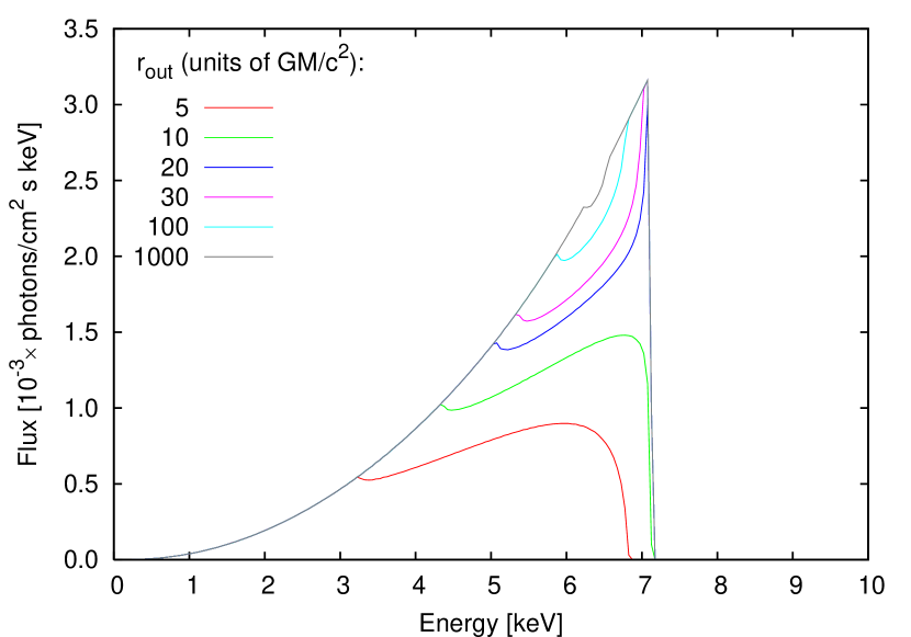
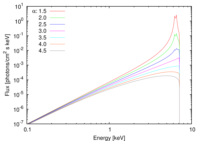
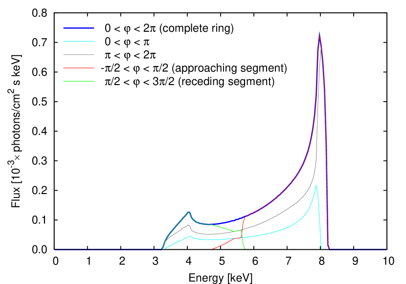
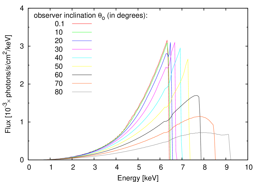
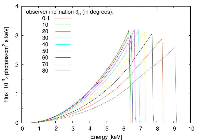
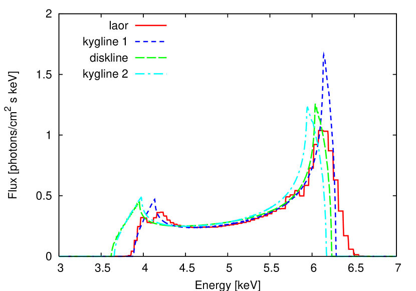
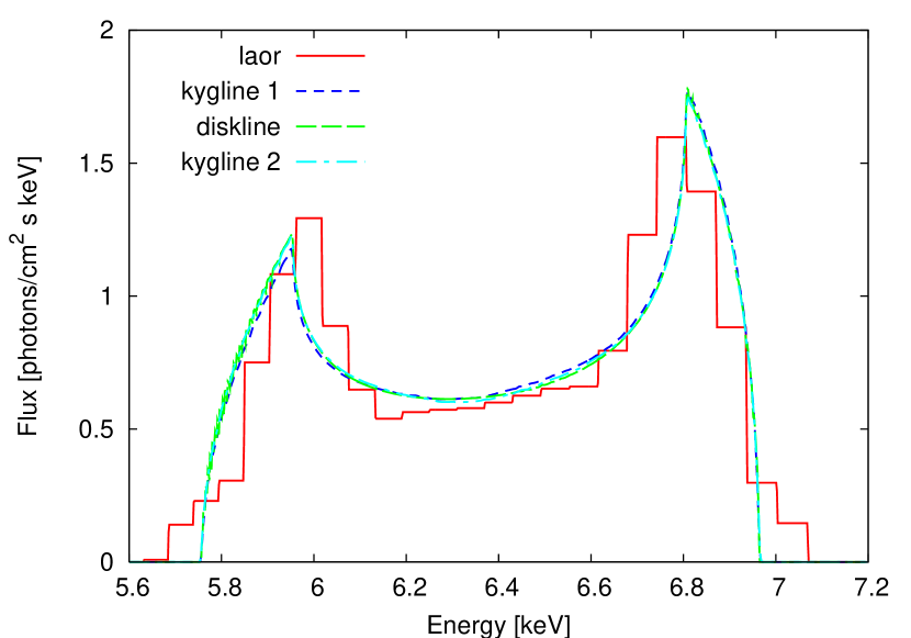
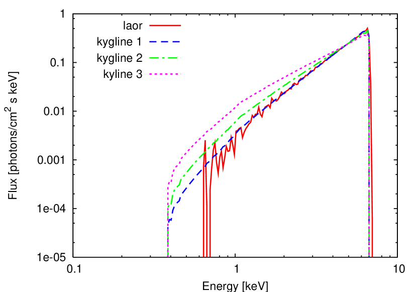
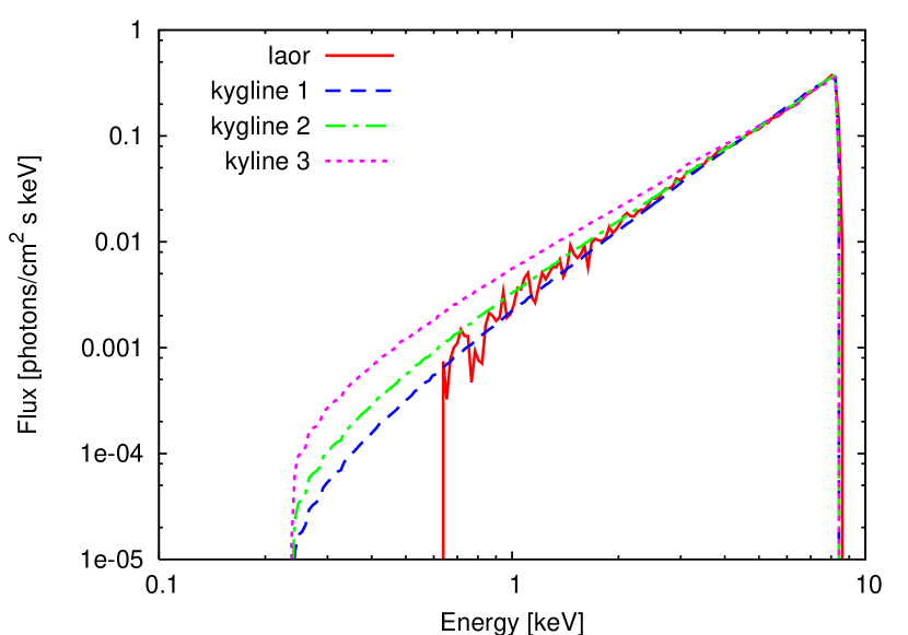
Results of an elementary code test are shown in Figures 7–9. The intrinsic emissivity was assumed to be a narrow gaussian line (width $\sigma\dot{=}0.42\,\mbox{FWHM}=5$ eV) with the amplitude decreasing $\propto{}r^{-\alpha}$ in the local frame co-moving with the disk medium. No background continuum is included here, so these lines can be compared with similar pure disk-line profiles obtained in previous papers (e.g. Laor 1991; Kojima 1991) which also imposed the assumption of axially symmetric and steady emission from an irradiated thin disk. Again, the intrinsic width of the line is assumed to be much less than the effects of broadening due to bulk Keplerian motion and the central gravitational field. Furthermore, Figures 10–11 compare model spectra of widely used xspec models.

Typically, the slope of the low-energy wing is rather sensitive do the radial dependence of emissivity. Notice also that the laor model gives zero contribution at energy below $0.1E_{\rm{}loc}=0.64\,$keV and its grid has only $35$ radial points distributed in the whole range $1.23{\leq}r{\leq}400$. Therefore, in spite of very efficient interpolation and smoothing of the final spectrum, the laor model does not accurately reproduce the line originating from a narrow ring. Also, dependence on the limb darkening/brightening cannot be examined with this model, because the form of directionality of the intrinsic emission is hard-wired in the code, together with the position of the inner edge at $r{\geq}r_{\rm{}ms}$.

The diskline model has been also used frequently in the context of spectral fitting, assuming a disk around a non-rotating black hole. This model is analytical, and so it has clear advantages in xspec. Notice, however, that the lensing effect is neglected. All this affects especially the spectrum near the black hole, where radiation is expected to be very anisotropic and flow lines non-circular.

Figure 10: Comparison of the output from xspec models for the disk-line problem: laor, diskline, and kygline (line 1 corresponds to the same limb-darkening law and $a=0.9982$ as in laor; line 2 assumes locally isotropic emission and $a=0$ as in diskline). Left panel: $\theta_{\rm{}o}=30^{\circ}$, $r_{\rm{}in}=6$, $r_{\rm{}out}=7$. Right panel: $\theta_{\rm{}o}=70^{\circ}$, $r_{\rm{}in}=100$, $r_{\rm{}out}=200$. Radial decay of intrinsic emissivity follows $\alpha=3$ power law. Default normalization of the model has been retained in this plot.

Figure 11: Comparison between the laor and kygline models. These plots are similar to previous figure, but in logarithmic scale and for three choices of the darkening law in kygline — (1) $I\propto 1+2.06\mu_{\rm{}loc}$; (2) $I={\rm{}const}$; (3) $I\propto\log(1+1/\mu_{\rm{}loc})$. Notice the impact on the calculated red-wing slope. Left panel: $\theta_{\rm{}o}=30^{\circ}$; Right panel: $\theta_{\rm{}o}=70^{\circ}$. In both panels, $r_{\rm{}in}=r_{\rm{}ms}$, $r_{\rm{}out}=400$, $a=0.9982$.

Appendix B Fast Model for Compton Reflection

In this Appendix we describe the Compton-reflection model hrefl. This model has been a part of the xspec distribution for some time. We have used similar approximation for the Compton-reflection in the disk to produce the relativistic version, kyhrefl.

The model has similar features to the well-known pexrav model (Magdziarz & Zdziarski 1995), which can often be prohibitively slow. There is a need for a fast reflection code for spectral fitting purposes, since the energy resolution of X-ray spectral data has been improved considerably in the last few years. Also, when convolving the reflection continuum with a kernel for relativistic energy shifting, computation speed is a critical factor. The price to pay is that hrefl makes use of a number of simplifying approximations. One of these is the elastic scattering approximation. Still, hrefl is accurate enough to be used for modelling data from observations of low-redshift sources with ASCA, Chandra, and XMM–Newton, where the source-frame spectrum does not extend beyond $\sim 15$ keV. (Notice, however, that this condition may be violated if the redshift of received photons is very large, e.g. near a black-hole horizon.) Another advantage of hrefl is that the model is completely analytic, and this is one of the major factors which makes it fast.

Below we give an outline of the model, providing important details of the adopted approximations, and a direct comparison with the pexrav model. A general description of the approach can be found in Basko (1978) along with any standard radiative transfer textbooks (e.g. Chandrasekhar 1960).

Figure 12: Left: Comparison between pexrav (solid) and hrefl*powerlaw (dashed) for two different inclination angles. Approximations are involved, making the model valid below $E\sim 15$ keV in the source rest-frame. Right: Comparison between the models kyhrefl (solid line) and hrefl*powerlaw (dashed line). Only the reflection component of the radiation flux due to the primary power-law continuum is plotted (in arbitrary units). Default model parameters were used with $\theta_{\rm{}o}=30^{\circ}$.

Let us consider a point source situated at a height $h$ above the center of an optically-thick disk with inner and outer radii $r_{\rm{}in}$ and $r_{\rm{}out}$ respectively. We define the cosines of the angles between the disk axis and lines connecting the inner and outer radii to the source as $\mu_{\rm min}$ and $\mu_{\rm max}$ respectively, where

$$\mu_{\rm min}=\frac{h}{\sqrt{r_{\rm{}in}^{2}+h^{2}}}\quad\mbox{and}\quad\mu_{\rm max}=\frac{h}{\sqrt{r_{\rm{}out}^{2}+h^{2}}}.$$ (B1)

The parameters actually required by the hrefl model are $\theta_{\rm min}=\arccos{\mu_{\rm min}}$ and $\theta_{\rm max}=\arccos{\mu_{\rm max}}$. In the approximation of an infinitely large disk with no hole at the center, $\theta_{\rm min}\rightarrow 0$ and $\theta_{\rm max}\rightarrow\pi/2$.

Now we adopt cylindrical coordinates with an origin coincident with the center of the disk face, and a set of rays emanating from the source and incident on the disk, making an angle $\arccos{\mu_{\rm{}i}}=\arccos{[h/\sqrt{h^{2}+r^{2}}]}$ with the disk normal at the point of interception. The incident specific intensity is $I_{\rm{}i}(r,\varphi)$. In the case of diffusive reflection from a plane-parallel atmosphere, the standard solution for the specific intensity of the reflected rays (as a function of energy, $\epsilon$) gives

$$I(\mu_{\rm{}r},\epsilon)=\frac{\lambda(\epsilon)}{4\pi}\;I_{\rm{}i}\,\mu_{\rm{}i}\;\frac{H[\mu_{\rm{}i},\lambda(\epsilon)]\,H[\mu_{\rm{}r},\lambda(\epsilon)]}{\mu_{\rm{}i}+\mu_{\rm{}r}}\quad[{\rm keV\ cm^{-2}\ s^{-1}\ sr^{-1}\ keV^{-1}}].$$ (B2)

Here, $\mu_{\rm{}r}$ is the cosine of the reflected rays with respect to the disk normal, $\lambda(\epsilon)$ is the single-scattering albedo (i.e. ratio of Thomson-scattering cross-section to the total scattering plus absorption cross-section), and $H[\mu,\lambda(\epsilon)]$ are the Chandrasekhar $H$-functions for isotropic scattering. The angles are to be evaluated in the frame co-rotating with the disk medium, which is particularly important in the relativistic version of the code when the bulk orbital motion is very rapid close to the black hole. The assumption of isotropic scattering is one of the simplifications we employ: at photon energies much less than the electron rest-mass, the angular dependence of photon-electron scattering is not very strong. The albedo is defined as

$$\lambda(\epsilon)=\frac{1.2\,\sigma_{\rm{T}}}{1.2\,\sigma_{\rm{T}}+\sigma_{\rm{abs}}(\epsilon)},$$ (B3)

where $\sigma_{\rm{T}}$ is the Thomson cross-section and $\sigma_{\rm{abs}}$ is the photoelectric absorption cross-section. The numerical factor $1.2$ accounts for electrons from ionized helium (those from heavier elements are neglected due to their smaller numbers).

Now we can reformulate equation (B2) in terms of actual fluxes. Let $N_{\rm{}d}(\epsilon)$ be the direct spectrum (${\rm photons\ cm^{-2}\ s^{-1}\ keV^{-1}}$) of an X-ray source, observed at a large distance $D$. Further, ${\rm{}d}F_{\rm{}i}$ denotes the energy flux within an energy interval ${\rm{}d}\epsilon$, which is incident on the face of the disk at radius $r$ from the disk center:

$${\rm{}d}F_{\rm{}i}=I_{\rm{}i}\,\mu_{\rm{}i}=\frac{4\pi D^{2}\epsilon\,N_{\rm{}d}(\epsilon)\,{\rm{}d}\epsilon}{4\pi(r^{2}+h^{2})}\;\mu_{\rm{}i}\quad[{\rm{}keV\ cm^{-2}\ s^{-1}}].$$ (B4)

The reflected flux that is received by a detector having an effective area $A$ from a disk surface element of area, $r\,{\rm{}d}r\,{\rm{}d}\varphi$, is then

$${\rm{}d}F_{\rm{}r}={\mu_{\rm{}r{}}}I({\mu_{\rm{}r{}}},\epsilon)\,r\,{\rm{}d}r\,{\rm{}d}\varphi\ \ 4\pi\left(\frac{A}{4\pi D^{2}}\right)\frac{1}{A}\quad[{\rm keV\ cm^{-2}\ s^{-1}}].$$ (B5)

Here, $4\pi(A/4\pi D^{2})$ is the solid angle subtended by the detector, $r=h\tan{\theta_{\rm{}i}}$, and ${\rm{}d}r=h\,{\rm{}d}\theta_{\rm{}i}/\mu_{\rm{}i}^{2}$.

Further, we denote the observed reflected spectrum $N_{\rm{}r}(\epsilon)$ $[{\rm photons\ \rm cm^{-2}\ s^{-1}\ keV^{-1}}]$. Since ${\rm{}d}F_{\rm{}r}=\epsilon\,{\rm{}d}N_{\rm{}r}(\epsilon)\,{\rm{}d}\epsilon\,{\rm{}d}{\mu_{\rm{}r{}}}$, we can substitute eq. (B4) into eq. (B2), then eq. (B2) into eq. (B5), and by integration over $\varphi$ from $0$ to $2\pi$ we find

$$N_{\rm{}r}(\epsilon)={\textstyle{\frac{1}{2}}}\lambda(\epsilon)\,N_{\rm{}d}(\epsilon)\int_{\mu_{\rm max}}^{\mu_{\rm min}}{\frac{{\mu_{\rm{}r{}}}\,{\rm{}d}\mu_{\rm{}i}}{\mu_{\rm{}i}+{\mu_{\rm{}r{}}}}}\,H[\mu_{\rm{}i},\lambda(\epsilon)]\,H[\mu_{\rm{}r},\lambda(\epsilon)].$$ (B6)

For the $H$-functions we use an approximation (Basko 1978) which is good to $\sim 8\%$ accuracy in the range $0\leq\lambda(\epsilon)\leq 1$ and $0\leq\mu\leq 1$:

$$H[\mu,\lambda(\epsilon)]\sim\frac{1+\sqrt{3}\,\mu}{1+\sqrt{3\left(1-\lambda(\epsilon)\right)}\;\mu}.$$ (B7)

Next, we notice that for a given $\lambda(\epsilon)$, $H[\mu_{\rm{}i},\lambda(\epsilon)]$ does not vary much, so we can bring it in front of the integral, replacing the exact formula with the mean over the range $\mu_{\rm{}i}=0$ to $\mu_{\rm{}i}=1$,

$$\bar{H}[\lambda(\epsilon)]=\int_{0}^{1}{H[\mu_{\rm{}i},\lambda(\epsilon)]\,{\rm{}d}\mu_{\rm{}i}}.$$ (B8)

For $\lambda(\epsilon)<1$ we obtain

$$\bar{H}[\lambda(\epsilon)]=\frac{1-\sqrt{1-\lambda(\epsilon)}}{\sqrt{3}\left(1-\lambda(\epsilon)\right)}\;\ln{\left[1+\sqrt{3\left(1-\lambda(\epsilon)\right)}\right]}+\frac{1}{\sqrt{1-\lambda(\epsilon)}},$$ (B9)

and for $\lambda(\epsilon)=1$

$$\bar{H}[\lambda(\epsilon)]=1+{\textstyle{\frac{1}{2}}}\,\sqrt{3}.$$ (B10)

Finally, we integrate equation (B6) over $\mu_{\rm{}i}$ to find

$$N_{\rm{}r}(\epsilon,\mu_{\rm{}r{}})={\textstyle{\frac{1}{2}}}\,N_{\rm{}d}(\epsilon,\mu_{\rm{}r{}})\,\lambda(\epsilon)\,\mu_{\rm{}r{}}\,\ln{\left(\frac{\mu_{\rm{}r{}}+\mu_{\rm min}}{\mu_{\rm{}r{}}+\mu_{\rm max}}\right)}\bar{H}[\lambda(\epsilon)]\,H[\mu_{\rm{}r{}},\lambda(\epsilon)].$$ (B11)

The function hrefl is encoded as a multiplicative component in xspec. When multiplied by the direct observed continuum, hrefl returns the reflected continuum, which is further multiplied by an effective reflection fraction, $R_{\rm{}c}$. The resulting contribution is added to the fraction $R_{\rm{}d}$ of direct continuum flux. In other words, $R_{\rm{}c}=1$ corresponds to $2\pi$ of the disk covering solid angle as seen by the X-ray source. Thus,

$$N_{\rm{}d}(\epsilon,\mu_{\rm{}r{}})\,\times\,\mbox{\sf{}hrefl}(\theta_{\rm min},\theta_{\rm max},\theta_{\rm{}o},R_{\rm{}c},R_{\rm{}d},\epsilon)=N_{\rm{}d}(\epsilon,\mu_{\rm{}r{}})\left[R_{\rm{}d}+R_{\rm{}c}\frac{N_{\rm{}r}(\epsilon,\mu_{\rm{}r{}})}{N_{\rm{}d}(\epsilon,\mu_{\rm{}r{}})}\right],$$ (B12)

where $\mu_{\rm{}r{}}$ has the meaning of observer inclination. The arguments of hrefl are the free parameters of the model (there are two more that are not listed explicitly here: they are the iron abundance relative to solar, and energy of the Fe-K edge). Notice that $R_{\rm{}c}$ and $R_{\rm{}d}$ are not independent, so no more than one of these two parameters is allowed to be free at any time of the fitting procedure. This way of coding the model is simply a matter of convenience for the user.

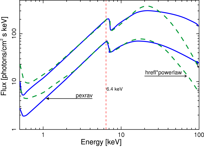
Fig. 12 (left panel) compares the pure reflection spectrum produced by hrefl with the pexrav model using an input power law (photon index $\Gamma=2$) for two inclination angles ($\mu_{\rm{}r}=0.95$ and $\mu_{\rm{}r}=0.1$, corresponding to $\theta_{\rm{}o}=18.2^{\circ}$ and $84.3^{\circ}$ respectively; pexrav does not allow for values of $\mu_{\rm{}r}<0.95$). In hrefl the parameters $\theta_{\rm min}$ and $\theta_{\rm max}$ were fixed at $0^{\circ}$ and $90^{\circ}$ respectively for the spectral fitting described in the present paper. Note that the relative iron abundance parameter for hrefl was set to $1.418=4.68\times 10^{-5}/3.3\times 10^{-5}$ because the two codes use different iron abundances.

Apart from the adopted approximations, additional discrepancies arise between hrefl and pexrav due to the use of different photoelectric absorption cross-sections (hrefl uses older versions of cross-section values than pexrav and the difference is visible at low energies of the spectrum). Between 1–15 keV the errors are less than 20% (much better accuracy than this value is achieved for the face-on inclinations). If the reflection continuum is combined with the direct continuum, for typical covering factors ($R_{\rm{}c}$), the errors below the Fe-K edge are practically negligible.

We conclude with the following concise summary of the approximations used in hrefl. The starting point of the model is the standard solution of the radiative transfer equation for reflection in a plane-parallel atmosphere. The simplifying assumptions are as follows. (i) Isotropic elastic scattering is assumed. (ii) Approximate analytical forms of the Chandrasekhar $H$-functions are used, as described in Basko (1978), but the accuracy of the approximate formulae is better than $\sim 8\%$. (iii) When integrating the incident continuum flux on the disk surface, the corresponding $H$-function is taken outside the integral and replaced with its mean value, $\bar{H}$.

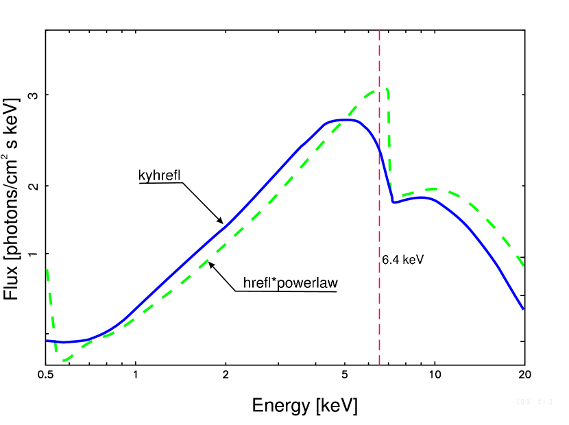
Fig. 12 (right panel) shows an example of the kyhrefl model spectrum, in which hrefl spectrum was smeared across the disk. kyhrefl can be interpreted as a Compton-reflection model for which the source of primary irradiation is near above the disk, in contrast to the lamp-post scheme with the source on axis. The approximations for Compton reflection used in hrefl (and therefore also in kyhrefl) are valid below $\sim 15$ keV in the source (and disk) rest-frame.

References

- (1) Arnaud K. A. 1996, in Astronomical Data Analysis Software and Systems V, eds. Jacoby G. & Barnes J., ASP Conf. Series 101, 17
- (2) Asaoka I. 1989, PASJ, 41, 763
- (3) Ballantyne D. R., Ross R. R., & Fabian A. C. 2001, MNRAS, 327, 10
- (4) Ballantyne, D. R., Vaughan, S., & Fabian, A. C. 2003, MNRAS, 342, 239
- (5) Bao G., Hadrava P., & Østgaard E. 1994, ApJ, 435, 55
- (6) Bao G., Hadrava P., Wiita P., & Xiong Y. 1997, ApJ, 487, 142
- (7) Basko M. M. 1978, ApJ, 223, 268
- (8) Beckwith K., & Done C. 2004, MNRAS, submitted (astro-ph/0402199)
- (9) Bromley B. C., Chen K., & Miller W. A. 1997, ApJ, 457, 57
- (10) Čadež A., Brajnik M., Gomboc A., Calvani M., & Fanton C. 2003, A&A, 403, 29
- (11) Chandrasekhar S. 1960, Radiative Transfer (New York: Dover)
- (12) Connors P. A., Stark R. F., & Piran T. 1980, ApJ, 235, 224
- (13) Cunningham C. T. 1975, ApJ, 202, 788
- (14) Czerny B., Różańska, Dovčiak M., Karas V., & Dumont A.-M. 2004, A&A, in press
- (15) Dabrowski Y., Fabian A. C., Iwasawa K., & Lasenby A. N., Reynolds C. S. 1997, MNRAS, 288, L11
- (16) Dabrowski Y., & Lasenby A. N. 2001, ApJ, 321, 605
- (17) de Felice F., Nobili L., & Calvani M. 1974, A&A, 30, 111
- (18) Done C., & Gierliński M. 2003, MNRAS, 342, 1041
- (19) Dovčiak M., Karas V., & Yaqoob T. 2004, in Proc. of the Workshop on Processes in the Vicinity of Black Holes and Neutron Stars (Opava 2003), eds. S. Hledík & Z. Stuchlík, in preparation
- (20) Dumont A.-M., Czerny B., Collin S., & Życki P. T. 2002, A&A, 387, 63
- (21) Fabian A. C., Iwasawa K., Reynolds C. S., & Young A. J. 2000, PASP, 112, 1145
- (22) Fabian A. C., Rees M. J., Stella L., & White N. E. 1989, MNRAS, 238, 729
- (23) Fabian C., & Vaughan S. 2003, MNRAS, 340, L28
- (24) Fabian A. C., Vaughan S., Nandra K., Iwasawa K., & Ballantyne D. R. et al. 2002, MNRAS, 335, L1
- (25) Fanton C., Calvani M., de Felice F., & Čadež A. 1997, PASJ, 49, 159
- (26) George I. M., Fabian A. C., 1991, MNRAS, 249, 352
- (27) Ghisellini G., Haardt F., Matt G., 1994, MNRAS, 267, 743
- (28) Gierliński M., Maciolek-Niedzwiecki A., & Ebisawa K. 2001, MNRAS, 325, 1253
- (29) Goyder R., & Lasenby A. N., 2004, MNRAS, in press (astro-ph/0309518)
- (30) Guainazzi G. 2003, A&A, 401, 903
- (31) Guainazzi G., et al. 1999, A&A, 341, L27
- (32) Hanisch R. J., et al. 2001, A&A, 376, 359
- (33) Hartnoll S. A., & Blackman E. G. 2001, MNRAS, 324, 257
- (34) Iwasawa K., et al. 1996, MNRAS, 282, 1038
- (35) Karas V., Vokrouhlický D., & Polnarev A. G. 1992, MNRAS, 259, 569
- (36) Kojima Y. 1991, MNRAS, 250, 629
- (37) Krolik J. 1999, ApJ, 515, L73
- (38) Krolik J., & Hawley J. F. 2002, ApJ, 573, 754
- (39) Laor A. 1991, ApJ, 376, 90
- (40) Lee J. C., et al. 2001, ApJ, 554, L13
- (41) Magdziarz P., & Zdziarski A. A. 1995, MNRAS, 273, 837
- (42) Martocchia A., Karas V., & Matt G. 2000, MNRAS, 312, 817
- (43) Martocchia A., Matt G., & Karas V. 2002a, A&A, 383. L23
- (44) Martocchia A., Matt G., Karas V., Belloni, T., & Feroci M. 2002b, A&A, 387, 215
- (45) Mason K. O., et al. 2003, ApJ, 582, 95
- (46) Matt G., Fabian A. C., & Ross R. R. 1993, MNRAS, 264, 839
- (47) Matt G., Perola G. C., Piro L., & Stella L. 1993a, A&A, 257, 63
- (48) Matt G., Perola G. C., & Stella L. 1993b, A&A, 267, 643
- (49) McClintock J. E., & Remillard R. A. 2003, in Compact Stellar X-ray Sources, eds. W. H. G. Lewin & M. van der Klis (astro-ph/0306213)
- (50) Miller J. M., et al. 2002a, ApJ, 578, 348
- (51) Miller J. M., et al. 2002b, ApJ, 577, L15
- (52) Miniutti G., Fabian A. C., Goyder R., & Lasenby A. N. 2003, MNRAS, 344, L22
- (53) Nandra K., George I. M., Mushotzky R. F., Turner T. J., & Yaqoob T. 1997, ApJ, 477, 602
- (54) Nayakshin S., & Kazanas D. 2002, ApJ, 567, 85
- (55) Pariev I., & Bromley C. 1998, ApJ, 508, 590
- (56) Pariev I., Bromley C., & Miller A. 2001, ApJ, 547, 649
- (57) Rauch K. P., & Blandford R. D. 1994, ApJ, 421, 46
- (58) Reynolds C. S., & Begelman M. C. 1997, ApJ, 488, 109
- (59) Reynolds C. S., & Nowak M. A. 2003, Phys. Rep., 377, 389
- (60) Reynolds C. S., Young A. J., Begelman M. C., & Fabian A. C. 1999, ApJ, 514, 164
- (61) Różańska A., Dumont A.-M., Czerny B., & Collin S. 2002, MNRAS, 332, 799
- (62) Ruszkowski M. 2000, MNRAS, 315, 1
- (63) Schneider P., Ehlers J., & Falco E. E., 1992, Gravitational Lenses (Springer, Berlin)
- (64) Schnittman J. D., & Bertschinger E. 2003, ApJ, submitted (astro-ph/0309458)
- (65) Semerák O., Karas V., & de Felice F. 1999, PASJ, 51, 571
- (66) Stella L. 1990, Nature, 344, 747
- (67) Tanaka Y., et al. 1995, Nature, 375, 659
- (68) Turner J., et al. 2002, ApJ, 574, L123
- (69) Viergutz S. U. 1991, A&A, 272, 355
- (70) Weaver K., & Yaqoob T. 1998, ApJ, 502, L139
- (71) Wilms J., et al. 2001, MNRAS, 328, L27
- (72) Yaqoob T., George I. M., Kallman T. R., Padmanabhan U., Weaver K. A., & Turner T. J. 2003, ApJ, 596, 85
- (73) Yaqoob T., & Padmanabhan U. 2004, ApJ, in press (astro-ph/0311551)
- (74) Zakharov A. F. 1994, MNRAS, 269, 283
- (75) Życki P., & Czerny B. 1994, MNRAS, 266, 653