The evolution of the luminosity functions in the FORS Deep Field from low to high redshift: I. The blue bands

We use the very deep and homogeneous I-band selected dataset of the FORS Deep Field (FDF) to trace the evolution of the luminosity function over the redshift range $0.5<z<5.0$. We show that the FDF I-band selection down to $I_{AB}=26.8$ misses of the order of 10 % of the galaxies that would be detected in a K-band selected survey with magnitude limit $K_{AB}=26.3$ (like FIRES). Photometric redshifts for 5558 galaxies are estimated based on the photometry in 9 filters (U, B, Gunn g, R, I, SDSS z, J, K and a special filter centered at 834 nm). A comparison with 362 spectroscopic redshifts shows that the achieved accuracy of the photometric redshifts is $\Delta z/(z_{spec}+1)\leq 0.03$ with only $\sim 1$% outliers. This allows us to derive luminosity functions with a reliability similar to spectroscopic surveys. In addition, the luminosity functions can be traced to objects of lower luminosity which generally are not accessible to spectroscopy. We investigate the evolution of the luminosity functions evaluated in the restframe UV (1500 Å and 2800 Å), u’, B, and g’ bands. Comparison with results from the literature shows the reliability of the derived luminosity functions. Out to redshifts of $z\sim 2.5$ the data are consistent with a slope of the luminosity function approximately constant with redshift, at a value of $-1.07\pm 0.04$ in the UV (1500 Å , 2800 Å) as well as u’, and $-1.25\pm 0.03$ in the blue (g’, B). We do not see evidence for a very steep slope ($\alpha\leq-1.6$) in the UV at $\langle z\rangle\sim 3.0$ and $\langle z\rangle\sim 4.0$ favoured by other authors. There may be a tendency for the faint-end slope to become shallower with increasing redshift but the effect is marginal. We find a brightening of M^∗ and a decrease of $\phi^{\ast}$ with redshift for all analyzed wavelengths. The effect is systematic and much stronger than what can be expected to be caused by cosmic variance seen in the FDF. The evolution of M^∗ and $\phi^{\ast}$ from $z=0$ to $z=5$ is well described by the simple approximations $M^{\ast}(z)=M^{\ast}_{0}+{a}\ln(1+z)$ and $\phi^{\ast}(z)=\phi^{\ast}_{0}(1+z)^{b}$ for $M^{\ast}$ and $\phi^{\ast}$. The evolution is very pronounced at shorter wavelengths ($a=-2.19$, and $b=-1.76$ for 1500 Å rest wavelength) and decreases systematically with increasing wavelength, but is also clearly visible at the longest wavelength investigated here ($a=-1.08$, and $b=-1.29$ for g’). Finally we show a comparison with semi-analytical galaxy formation models.

1 Introduction

Observational constraints on galaxy formation have improved significantly over the last years and it has become possible to study the evolution of global galaxy properties up to very high redshifts. A crucial step to probe the properties of galaxies up to the highest redshifts was the work of Steidel & Hamilton (1993) and Steidel et al. (1996) who used color selection to discriminate between low redshift and high redshift galaxies. Although the Lyman-break technique is very efficient in selecting high redshift galaxies (see Blaizot et al. 2003 for a detailed discussion) with a minimum of photometric data, it has the disadvantage that it does not sample galaxies homogeneously in redshift space and may select against certain types of objects. With the advent of deep multi-band photometric surveys (Hubble Deep Field North (HDFN; Williams et al. 1996), NTT SUSI deep Field (NDF; Arnouts et al. 1999), Hubble Deep Field South (HDFS; Williams et al. 2000; Casertano et al. 2000), Chandra Deep Field South (CDFS; Arnouts et al. 2001), William Herschel Deep Field (WHDF; McCracken et al. 2000; Metcalfe et al. 2001), Subaru Deep Field/Survey (SDF; Maihara et al. 2001; Ouchi et al. 2003a),

The Great Observatories Origins Deep Survey (GOODS; Giavalisco et al. 2004)) the photometric redshift technique (essentially a generalization of the drop-out technique) has increasingly been used to identify high-redshift galaxies. Several methods have been described in the literature to derive photometric redshifts (Baum, 1962; Koo, 1985; Brunner et al., 1999; Fernández-Soto et al., 1999; Benítez, 2000; Le Borgne & Rocca-Volmerange, 2002; Firth et al., 2003).

Based on either spectroscopic redshifts, drop-out techniques, or photometric redshifts, it has been possible to derive luminosity functions at different redshifts in the ultraviolet (UV) (Treyer et al., 1998; Steidel et al., 1999; Cowie et al., 1999; Adelberger & Steidel, 2000; Cohen et al., 2000; Sullivan et al., 2000; Ouchi et al., 2001; Poli et al., 2001; Wilson et al., 2002; Wolf et al., 2003; Rowan-Robinson, 2003; Kashikawa et al., 2003; Ouchi et al., 2003a; Iwata et al., 2003) and in the blue bands (Lilly et al., 1995; Heyl et al., 1997; Lin et al., 1997; Sawicki et al., 1997; Small et al., 1997; Zucca et al., 1997; Loveday et al., 1999; Marinoni et al., 1999; Fried et al., 2001; Cross & Driver, 2002; Im et al., 2002; Marinoni et al., 2002; Norberg et al., 2002; Bell et al., 2003; de Lapparent et al., 2003; Liske et al., 2003; Poli et al., 2003; Pérez-González et al., 2003). Within the uncertainties given by IMF and dust content, the flux in the UV allows to trace the star formation rate (SFR; Madau et al. 1998) in the galaxies, while the optical luminosities provide constraints on more evolved stellar populations (Franx et al., 2003).

Locally, the 2dF Galaxy Redshift Survey (2dFGRS; Colless et al. 2001), the Sloan Digital Sky Survey (SDSS; Stoughton et al. 2002) and the 2MASS survey (Jarrett et al., 2000) have provided superb reference points for galaxy luminosity functions over a large wavelength range (see Norberg et al. 2002 for 2dFGRS, Blanton et al. 2001, 2003 for the SDSS, and Kochanek et al. 2001; Cole et al. 2001 for 2MASS).

In parallel to the observational effort, theoretical models have been developed within the framework of the cold dark matter cosmology. Most notably, semi-analytic models (SAMs) (Kauffmann et al., 1993; Cole et al., 1994; Somerville & Primack, 1999; Kauffmann et al., 1999; Poli et al., 1999; Wu et al., 2000; Cole et al., 2000; Menci et al., 2002, 2003) and simulations based on smoothed-particle hydrodynamics (SPH) (Davé et al., 1999; Weinberg et al., 2002; Nagamine, 2002; Nagamine et al., 2003) have made testable predictions. Starting with the mass function of dark matter halos and their merging history, SAMs use simplified recipes to describe the baryonic physics (gas cooling, photoionization, star formation, feedback processes, etc., see Benson et al. 2003) to derive stellar mass and luminosity functions.

Ideally, a comparison between observations and models should be done with deep multiwavelengths datasets that also cover a large area. The dataset has to be sufficiently deep in order to be able to derive the faint-end slope of the luminosity function. On the other hand, one also needs as large an area as possible to overcome cosmic variance and to quantify the density of rare bright galaxies, which define the cut-off of the luminosity function.

The FORS Deep Field (Heidt et al., 2003) has a depth close to the HDFs but an area of 8 – 10 times the area of the HDFN. This depth allows us to detect galaxies at $z>2$ which would be missed by Lyman-break studies which usually reach only $R_{AB}<25.5$ (see also Franx et al. 2003 and van Dokkum et al. 2003).

Very reliable photometric redshifts are crucial for the analysis of the evolution of the luminosity functions in the FDF. Photometric redshifts have been determined with a template matching algorithm described in Bender et al. (2001) that applies Bayesian statistics and uses semi-empirical template spectra matched to broad band photometry. We achieved an accuracy of $\Delta z/(z_{spec}+1)\leq 0.03$ with only $\sim 1$% extreme outliers (numbers based on a comparison with 362 spectroscopic redshifts). Redshifts of galaxies that are several magnitudes fainter than typical spectroscopic limits could be determined reliably and thus allowed better constraints on the faint-end slope of the luminosity functions.

In this paper we present the redshift evolution of the luminosity function evaluated in the restframe UV-range (1500 Å, 2800 Å), u’ (SDSS), B, and g’ (SDSS) bands in the redshift range $0.5<z<5.0$. Luminosity functions at longer wavelengths as well as the evolution of the luminosity density and the star formation rate will be presented in future papers (Gabasch et al., in preparation). We provide a short description of the FDF in Sect. 2 where we also present the selection criteria of our galaxies. In Sect. 3 we investigate possible selection effects due to our purely I-band selected catalogue. In Sect. 4 we discuss the accuracy of the photometric redshifts as well as the redshift distribution of the selected galaxies. In Sect. 5 and in the Appendix we show luminosity functions at different wavelengths and redshifts. In Sect. 6, a parameterization of the redshift evolution of the Schechter (Schechter, 1976) parameters M^∗ and $\phi^{\ast}$ is given. We compare our results with previous observational results in Sect. 7, and with model predictions in Sect. 8, before we summarize this work in Sect. 9.

We use AB magnitudes and adopt a $\Lambda$ cosmology throughout the paper with $\Omega_{M}=0.3$, $\Omega_{\Lambda}=0.7$, and $H_{0}=70\,\mathrm{km}\,\mathrm{s}^{-1}\,\mathrm{Mpc}^{-1}$.

2 The FORS deep field

The FORS Deep Field (Appenzeller et al., 2000) is a multi-color photometric and spectroscopic survey of a $7^{\prime}\times 7^{\prime}$ region near the south galactic pole including the QSO Q 0103-260 at redshift $z=3.36$. The data have been taken with FORS1 and FORS2 at the ESO VLT and SofI at the NTT.

The data in the U, B, g, R, I, J and Ks filters were reduced and calibrated (including the correction for galactic extinction) as described in Heidt et al. (2003). The reduction of the images in the z-band and the special filter centered at 834 nm follows the same recipe, except for additional de-fringing in the z-band.

The images were stacked with weights to get optimal signal to noise for point-like faint objects. The formal 50% completeness limits for point sources are 26.5, 27.6, 26.9, 26.9, 26.8, $\sim 25.5$, $\sim 25.8$, 23.8, 22.6 in U, B, g, R, I, 834 nm, z, J and Ks, respectively. The seeing varied from 0.5 arcsec in the I and z band to 1.0 arcsec in the U-band. Because the depth of the images decreases towards the borders, we limited our analysis to the inner 39.81 arcmin² of our field. The signal-to-noise ratio (S/N) in this ‘deep’ region is at least 90 % of the best S/N in every filter. This prevents a possible bias of the photometric redshifts (see Sect. 4) due to a not completely homogeneous dataset.

Object detection was done in the I-band image using SExtractor (Bertin & Arnouts, 1996), and the catalogue for this ‘deep’ part of the FDF includes 5636 objects. To avoid contamination from stars, we rely on three sources of information: The star-galaxy classifier of the detection software SExtractor, the goodness of fit for galaxy objects of the photometric redshift code and, if available, on the spectroscopic information. We first exclude all bright ($I<22^{m}$) starlike objects (SExtractor star galaxy classifier $>0.95$). Then we exclude all objects whose best fitting stellar spectral energy distribution (SED) – according to the photometric redshift code – gives a better match to the flux in the different wavebands than any galaxy template ($2\ \chi_{star}^{2}<\chi_{galaxy}^{2}$). These objects are subsequently flagged as star and removed from our catalogue. Further inspection of the images confirms, that none of these flagged objects are extended. Finally, we reject all objects spectroscopically classified as stars. We checked the influence of misidentified or missed stars on the luminosity functions. If stars are fitted by galaxy templates their redshifts are mostly very small ($z<0.15$, especially if they are G and K stars) and, therefore, did not enter the analysis. M stars interpreted as galaxies tend to be distributed more evenly in redshift space but they do not contribute significantly to the number density in any redshift interval. Even if all stars were included as galaxies in the sample, they would not affect the derived luminosity functions at a noticeable level.

In total 78 objects were classified as stars and removed from our sample. Our final I-band selected catalogue comprises therefore 5558 objects.

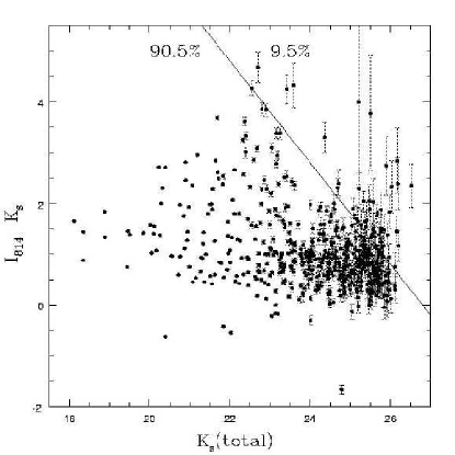
Figure 1: $I_{814}-K_{s}$ versus $K_{s}$ color-magnitude relation for $K_{s}$-selected objects of the HDF-S as given by Labbé et al. (2003). Following Labbé et al. (2003) only sources with a minimum of 20% of the total exposure time in all bands are included and shown as filled symbols. Colors are plotted with $1\sigma$ error bars. The solid line corresponds to the limiting magnitude of the FDF (I=26.8). Only the objects on the right of the solid line are beyond our I-band limit.

3 I selection versus K selection

We use the ultradeep near-infrared ISAAC observations of the Hubble Deep Field South (Labbé et al., 2003) for a more quantitative analysis of possible selection effects between K and I band selected samples.

In Fig. 1 we show the $I_{814}-K_{s}$ versus $K_{s}$ color-magnitude relation for $K_{s}$-selected objects of the HDF-S as given by Labbé et al. (2003) (data were taken from: http://www.strw.leidenuniv.nl/$\sim$fires/). Following Labbé et al. (2003), only sources with a minimum of 20% of the total exposure time in all bands are included and shown as filled symbols. Colors are plotted with $1\sigma$ error bars. The solid line corresponds to the 50 % completeness limiting magnitude of the FDF in the I-band ($I\sim 26.8$). The figure clearly shows, that although we selected in I, we miss only about 10 % of the objects that would have been detected in deep K-band images (with a 50 % completeness limiting magnitude of $K_{AB}\sim 26.3$). All objects on the left of the solid line would have been detected in the I-selected FDF catalogue as well. Therefore we conclude that only a small fraction ($\sim 10$ %) of galaxies is missed in deep I-band selected samples relative to deep K-band selected samples, provided the I-band images are about 0.5 AB-magnitudes deeper than the K-band images. Of course, this holds only for galaxies at redshift below 6. At higher redshifts no signal is detectable in the I-band, due to the Lyman break and intervening intergalactic absorption.

Another indication that we are unlikely to miss a large population of high redshift red galaxies comes from Fig. 4 (left panel). Out to redshifts of about 1.5, red galaxies define the bright end of the luminosity function. Beyond $z\sim 1.5$ bluer star-forming galaxies take over. Red galaxies could still be detected at $z>1.5$ but seem to be largely absent. In any case, even if we missed a few objects, the evolution of luminosity functions that we discuss below will not be affected.

As a side remark we note that also a B-band selected FDF catalogue delivers similar conclusions on the evolution of the luminosity functions out to redshift $\sim 3$. Again, above this redshift no signal is detectable in the B-band due to the Lyman break and intervening intergalactic absorption.

4 Photometric redshifts

Figure 2: Comparison of spectroscopic (Noll et al., 2003; Böhm et al., 2003) and photometric redshifts for different galaxy types and quasars in the FDF (362 objects).

Figure 3: Left panel: Histogram of the reduced $\chi^{2}$ for all galaxies in the FDF as obtained for the best fitting template and redshift. The dotted vertical line indicates the median reduced $\chi^{2}$. Right panel: Histogram of the photometric redshift errors. The error distribution can be approximated by a Gaussian centered at 0.006 with an rms of 0.028 (dotted line).

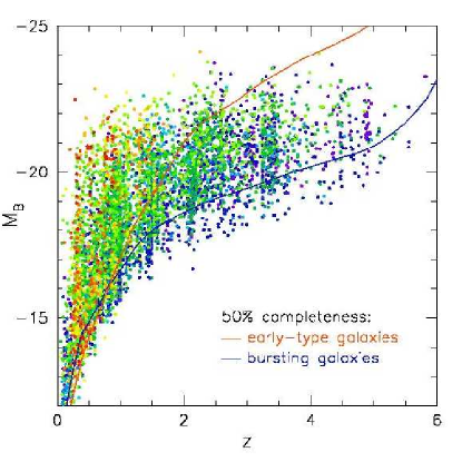
Figure 4: Left panel: Absolute B magnitudes of galaxies in the FDF against redshift. Colors indicate spectral types (red to blue: old to young). The two lines indicate the 50% completeness limit for a red and a blue spectral energy distribution corresponding to an I-band limiting magnitude of 26.8. Right panel: Redshift number distribution of all galaxies in the FDF sample. The clustering observed in photometric redshift space (both panels) is probably mostly real, as we see clustered spectroscopic redshifts at $z=0.22$, $z=0.33$, $z=0.39$, $z=0.45$, $z=0.77$, $z=2.35$ and possibly at $z=0.95$, $z=3.15$, and $z=3.4$.

A brief summary of the photometric redshift technique used to derive the distances to the galaxies in the FDF can be found in Bender et al. (2001), a more detailed description will be published in a future paper (Bender et al. 2004). Well determined colors of the objects which implies very precise zeropoints in all filters are crucial to derive accurate photometric redshifts. Therefore we checked and fine-tuned the calibration of our zeropoints by means of color-color plots of stars. We compared the colors of FDF stars with the colors of stellar templates from the library of Pickles (1998) converted to the FORS filter system. In general, corrections to the photometric zeropoints of only a few hundredth of a magnitude were needed to obtain an optimal match to the stars and best results for the photometric redshifts. In order to avoid contamination from close-by objects, we derived object fluxes for a fixed aperture of 1.5” ($1.5\times$ seeing) from images which had been convolved to the same point spread function. A redshift probability function P(z) was then determined for each object by matching the object’s fluxes to a set of 30 template spectra redshifted between $z=0$ and $z=10$ and covering a wide range of ages and star formation histories. As templates we used (a) local galaxy templates from Mannucci et al. (2001), and Kinney et al. (1996) and (b) semi-empirical templates more appropriate for modest to high redshift galaxies. The semi-empirical templates were constructed by fitting combinations of theoretical spectral energy distributions of different ages from Maraston (1998) and Bruzual & Charlot (1993) with variable reddening (Kinney et al., 1994) to the observed broad band colors of about 100 galaxies in the Hubble Deep Field and about 180 galaxies from the FDF with spectroscopic redshifts. The remaining 180 galaxies in the FDF with spectroscopic redshift were used as an independent control sample. Lyman forest absorption was parameterized following Madau (1995) and references therein.

In Fig. 2 we compare the photometric and spectroscopic redshifts of 362 galaxies and QSOs in the FDF (see Noll et al. 2003; Böhm et al. 2003 for the spectroscopic redshifts). The agreement is very good and we have only 6 outliers with a redshift error larger than $\Delta z>1$ among 362 objects. Three of the outliers are quasars or galaxies with a strong power-law AGN component (crosses). The others are very blue objects with an almost feature-less continuum (triangles). Fig. 3 (left panel) presents the $\chi^{2}$ distribution for the best fitting template and photometric redshifts. Note that to calculate the $\chi^{2}$, we have used the observational photometric errors and, in addition, have assumed that the templates have an intrinsic uncertainty of typically 5% in the optical bands and 20% in the infrared bands. The larger errors for the near-IR take into account the slightly lower quality of the infrared data if compared to the optical. Allowing for this intrinsic uncertainty turns a discrete set of templates into a template-continuum. Observational errors and intrinsic ‘errors’ were added in quadrature. The median value of the reduced $\chi^{2}$ is below 1.7 and demonstrates that the galaxy templates describe the vast majority of galaxies in the FDF very well. The right panel of Fig. 3 shows the distribution of the redshift errors. It is nearly Gaussian and scatters around zero with an rms error of $\Delta z/(z_{spec}+1)\approx 0.03$. In Fig. 4 (left panel), we plot the absolute B-band magnitudes against the photometric redshifts of the objects. Colors from red to blue indicate increasingly bluer spectral energy distributions. The two lines indicate the 50% completeness limit for a red and a blue spectral energy distribution corresponding to an I-band limiting magnitude of 26.8. The redshift histogram of all objects in the FDF is shown in the right panel of Fig. 4 (see also Table 1). Most if not all peaks in the distribution are due to real clustering in redshift space. From the 362 spectroscopic redshifts, we have identified clusters, groups or filaments of galaxies with more than 10 identical or almost identical redshifts at $z=0.22$, $z=0.33$, $z=0.39$, $z=0.45$, $z=0.77$, $z=2.35$. Other structures (with only a few identical spectroscopic redshifts) are possibly present at $z=0.95$, $z=3.15$, and $z=3.4$.

Table 1: Galaxy distribution in the FDF for the redshift intervals used for computing the luminosity function. Note that we derive the luminosity function in all redshift bins, but exclude the lowest ($z<0.45$) and highest redshift bin ($z>5.01$) from our analysis of the luminosity function evolution, since the lowest redshift bin corresponds to a too small volume while the $z>5.01$ bin suffers from incompleteness.

redshift	number	fraction
interval	of galaxies	of galaxies
0.00 - 0.45	808	14.54 %
0.45 - 0.81	998	17.96 %
0.81 - 1.11	885	15.92 %
1.11 - 1.61	898	16.16 %
1.61 - 2.15	504	9.07 %
2.15 - 2.91	746	13.42 %
2.91 - 4.01	549	9.88 %
4.01 - 5.01	150	2.70 %
$>5.01$	18	0.32 %
unknown	2	0.04 %

5 Luminosity functions

5.1 The method

We compute the absolute magnitudes of our galaxies using the I-band selected catalogue as described in Sect. 2 and the photometric redshifts described in Sect. 4. To derive the absolute magnitude for a given band we use the best fitting SED as determined by the photometric redshift code and convolve it with the appropriate filter function. As the SED fits all 9 observed-frame wavebands simultaneously, possible systematic errors which could be introduced by using K-corrections applied to a single observed magnitude are reduced. Since the photometric redshift code works with 1.5” aperture fluxes, we only need to correct to total luminosities by applying an object dependent scale factor. For this scale factor we used the ratio of the I-band aperture flux to the total flux as provided by SExtractor (MAG_APER and MAG_AUTO). We have chosen the I-band because (a) our I-band data are very deep, (b) all objects were detected and selected in the I-band, and (c) high redshift galaxies have only poorly determined or no flux at shorter wavelengths. This procedure may introduce a slight bias, as galaxies are more compact or knotty in the rest-frame UV bands (tracing HII regions) than at longer wavelengths. However, scaling factors derived in the deep B-band turned out to be similar (for low enough redshifts).

In a given redshift interval, the luminosity function is computed by dividing the number of galaxies in each magnitude bin by the volume $V_{\mathrm{bin}}$ of the redshift interval. To account for the fact that some fainter galaxies are not visible in the whole survey volume we perform a $V/V_{max}$ (Schmidt, 1968) correction. Using the best fitting SED we calculate the maximum redshift $z_{max}$ at which the object could have been observed given the magnitude limit of our field. We weight each object by $V_{bin}/V_{max}$ where $V_{bin}$ is the volume of our redshift bin enclosed by $z_{low}$ and $z_{high}$ and $V_{max}$ is the volume enclosed between $[z_{low},\textrm{min}(z_{high},z_{max})]$.

To derive reliable Schechter parameters we limit our analysis of the luminosity function to the bin where the $V/V_{max}$ begins to contribute at most by a factor of 3 (we also show the uncorrected luminosity function in the various plots as open circles). The redshift binning was chosen such that we have good statistics in every redshift bin and that the influence of redshift clustering was minimized. The redshift binning and the number of galaxies in every bin is shown in Table 1.

The errors of the luminosity functions are calculated by means of Monte-Carlo simulations as follows. The photometric redshift code provides redshift probability distributions P(z) for each single galaxy. In each Monte-Carlo realization, we randomly pick a new redshift for each object from a sample of redshifts distributed like P(z) and calculate the corresponding luminosity. This we repeat 250 times which allows us to derive the dispersion of the galaxy number density $\phi(M,z)$ for each magnitude and redshift bin due to the finite width of P(z) for each galaxy. The total error in $\phi$ is finally obtained by adding in quadrature the error from the Monte-Carlo simulations and the Poissonian error derived from the number of objects in the bin.

Photometric redshift errors may, in principle, affect the shape of the luminosity function at the bright end: By scattering objects to higher redshifts they let the steep fall-off at high luminosities appear shallower (Drory et al., 2003). However, in the case of the FDF the redshift errors are so small that the influence on the shape of the luminosity function is negligible.

5.2 The slope of the luminosity function

Table 2: Slope of the luminosity function for all wavelengths and all redshifts as derived from 3-parameter Schechter fits.

$z$	$\alpha$ (1500 Å)	$\alpha$ (2800 Å)	$\alpha$ (u’)	$\alpha$ (g’)	$\alpha$ (B)
$[0.45,0.81]$	$-$1.14 (+0.08 $-$0.07)	$-$1.23 (+0.08 $-$0.07)	$-$1.27 (+0.06 $-$0.05)	$-$1.34 (+0.05 $-$0.03)	$-$1.30 (+0.05 $-$0.03)
$[0.81,1.11]$	$-$0.96 (+0.13 $-$0.10)	$-$0.99 (+0.10 $-$0.08)	$-$0.93 (+0.09 $-$0.07)	$-$1.16 (+0.07 $-$0.04)	$-$1.21 (+0.07 $-$0.04)
$[1.11,1.61]$	$-$1.05 (+0.18 $-$0.16)	$-$1.03 (+0.13 $-$0.11)	$-$0.95 (+0.10 $-$0.09)	$-$1.13 (+0.11 $-$0.09)	$-$1.12 (+0.09 $-$0.07)
$[1.61,2.15]$	$-$0.81 (+0.48 $-$0.45)	$-$0.97 (+0.32 $-$0.28)	$-$0.80 (+0.31 $-$0.27)	$-$1.29 (+0.24 $-$0.21)	$-$1.33 (+0.27 $-$0.20)
$[2.15,2.91]$	$-$0.38 (+0.21 $-$0.15)	$-$0.67 (+0.18 $-$0.15)	$-$0.70 (+0.16 $-$0.16)	$-$0.89 (+0.22 $-$0.15)	$-$0.70 (+0.24 $-$0.21)
$[2.91,4.01]$	$-$0.98 (+0.28 $-$0.24)	$-$0.95 (+0.19 $-$0.17)	$-$1.25 (+0.19 $-$0.14)	$-$1.24 (+0.23 $-$0.20)	$-$1.30 (+0.27 $-$0.20)
$[4.01,5.01]$	$-$0.77 (+0.38 $-$0.26)	$-$1.03 (+0.46 $-$0.35)	$-$1.09 (+0.54 $-$0.27)	$-$1.18 (+0.37 $-$0.21)	$-$0.77 (+0.49 $-$0.39)

We first investigate the redshift evolution of the faint-end slope of the luminosity function by fitting all three parameters of the Schechter function (M^∗, $\phi^{\ast}$, and $\alpha$). The best fitting $\alpha$ and the corresponding $1\sigma$ errors for all wavebands and redshifts are listed in Table 2.

Despite of the depth of the FDF, Table 2 shows that it is only possible to obtain reasonably tight constraints on the slope $\alpha$ for $z<1.5$. In addition, strong parameter coupling is observed between M^∗ and $\alpha$ (see Fig. 25 in the Appendix C). We find only marginal evidence for a change of $\alpha$ with redshift for all wavebands. The lowest redshift bin ($0.15<z<0.45$), which we excluded from the fit because of poor number statistics in bright objects, generally shows the steepest faint-end slope. Beyond redshift 0.5, all data are consistent with a constant and shallow faint-end slope.

We obtain as best error-weighted values for all redshifts between 0.45 and 5.0 the numbers given in Table 3 (upper part), assuming that $\alpha$ does not depend on redshift. The slopes in the 1500 Å, 2800 Å, and u’ band are very similar. The same applies for the slope in the g’ and B band. Therefore, we combined the data for the 1500 Å, 2800 Å, and u’ band as well as for the g’ and B band and derived combined slopes with an error weighted fit to the data of Table 2. The results are also listed in Table 3 (lower part).

Table 3: Slope $\alpha$ of the luminosity functions for the different wavebands as determined from an error-weighted fit to the data in Table 2 under the assumption that $\alpha(z)=\mathrm{const.}$ (upper part). In the lower part of the Table we show the best values of $\alpha$ after combining the UV bands and the blue optical bands.

filter	$\alpha(z)=const$
1500 Å	$-1.01\pm 0.08$
2800 Å	$-1.06\pm 0.07$
u’	$-1.10\pm 0.08$
g’	$-1.26\pm 0.04$
B	$-1.24\pm 0.04$
1500 Å & 2800 Å & u’	$-1.07\pm 0.04$
g’ & B	$-1.25\pm 0.03$

Almost all of the slopes listed in Table 2 are compatible within $2\sigma$ with the slopes in Table 3. Therefore, we fixed the slope to these values for further analysis. This simplification is also justified by the fact that for all subsequent fits with fixed slope the reduced $\chi^{2}$ was generally close to 1.

As a last test, we investigated the influence of the redshift binning on the slope $\alpha$. We enlarged our first two redshift bins to $0.41<z\leq 0.91$ (1433 galaxies) and $0.91<z\leq 1.61$ (1438 galaxies) which allowed us to determine luminosity functions with lower errors in all wavebands. The slopes derived in these two larger bins were compatible with our previously derived fixed slope in every waveband.

5.3 The restframe luminosity functions

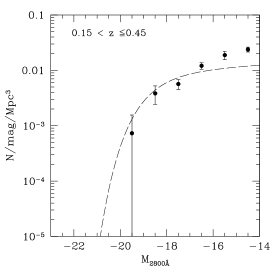
Figure 5: Luminosity functions at 2800 Å from low redshift ($\langle z\rangle=0.3$, upper left panel) to high redshift ($\langle z\rangle=5.5$, lower right panel). The filled (open) symbols show the luminosity function corrected (uncorrected) for $V/V_{max}$. The fitted Schechter functions for a fixed slope $\alpha$ are shown as solid lines. Note that we only fit the luminosity functions from $\langle z\rangle=0.6$ to $\langle z\rangle=4.5$. The parameters of the Schechter functions are given in Table 6. The Schechter fit for redshift $\langle z\rangle=0.6$ is indicated as dashed line in all panels.

Figure 6: Luminosity functions in the g’-band from low redshift ($\langle z\rangle=0.3$, upper left panel) to high redshift ($\langle z\rangle=5.5$, lower right panel). The filled (open) symbols show the luminosity function corrected (uncorrected) for $V/V_{max}$. The fitted Schechter functions for a fixed slope $\alpha$ are shown as solid lines. Note that we only fit the luminosity functions from $\langle z\rangle=0.6$ to $\langle z\rangle=4.5$. The parameters of the Schechter functions can be found in Table 8. The dotted line represents the local g’-band luminosity function derived from the SDSS (Blanton et al., 2001). The Schechter fit for redshift $\langle z\rangle=0.6$ is indicated as dashed line in all panels.

In this section we analyze the luminosity function in the UV (1500 Å, 2800 Å), u’, g’, and B band by means of a Schechter function fit with fixed slope (see Sect. 5.2).

In the UV, we evaluate the luminosity function in two rectangular filters centered at $1500\pm 100$ Å and $2800\pm 100$ Å. There are three reasons to analyze both wavelengths. First, for our lowest redshift bin ($\langle z\rangle\sim 0.6$) the restframe magnitude derived at 2800 Å is more robust than the one at 1500 Å because the restframe wavelength of 2800 Å corresponds to the observed U and does not need extrapolation to shorter wavelength. Second, we also include the 1500 Å luminosity function as it corresponds to a frequently used reference wavelength and is very well determined beyond redshifts of 2.5. Third, we want to show that the galaxy luminosity functions at both wavelengths are very similar and show the same redshift evolution.

Figure 7: $1\sigma$ and $2\sigma$ confidence levels in Schechter parameter space for the different redshift bins, labeled by their mean redshift. A Schechter function with a fixed slope (see Table 3) has been fitted to the luminosity function at 1500 Å (upper left panel), 2800 Å (upper right panel), in the u’-band (lower left panel) and in the g’-band (lower right panel). The parameters of the Schechter function can be found in Table 5, Table 6 Table 7 and Table 8.

In the optical bands, we calculated the evolution of the luminosity functions in the u’ and g’ bands (g’ of SDSS, see Fukugita et al. 1996, not to be confused with Gunn g which was part of the filter set with which we observed the FDF). Because many authors have already published luminosity functions in the Johnson B-band, we include also this filter in our analysis.

In Figs. 5 and 6 we present the luminosity functions at 2800 Å and in the g’ band, while the results at 1500 Å as well as for the u’ and B bands can be found in Figs. 14, 15 and 16 in appendix A. The filled (open) symbols denote the luminosity function with (without) completeness correction.

Even without fitting Schechter functions to the data, it is obvious that there is strong evolution in characteristic luminosity and number density between redshifts 0.6 and 4.5.

The solid lines show the Schechter function fitted to the luminosity function. The best fitting Schechter parameter, the redshift binning as well as the reduced $\chi^{2}$ are also listed. The reduced $\chi^{2}$ are quite good for all but one redshift bin ($2.15<z\leq 2.91$). The slope we adopted is not suitable for that bin and increases the $\chi^{2}$. The depth of the FDF allows us to trace the luminosity function over a relatively large magnitude range. Even in our highest redshift bin ($4.01<z\leq 5.01$) the luminosity function spans an interval of 4 magnitudes.

In Fig. 7 we show the $1\sigma$ and $2\sigma$ confidence contours of M^∗ and $\phi^{\ast}$ for the different redshift bins, illustrating the correlation of the two Schechter parameters. The contours correspond to $\Delta\chi^{2}=2.30$ and $\Delta\chi^{2}=6.17$ above the minimum $\chi^{2}$. The best fitting Schechter parameters and their $1\sigma$ errors are summarized in Tables 5, 6, 7, 8 and 9 for the 1500 Å, 2800 Å, u’, g’ and B bands, respectively. The $1\sigma$ errorbars of the single parameters are derived from the projections of the two-dimensional contours using $\Delta\chi^{2}=1$.

We find a systematic brightening of M^∗ and a systematic decrease of $\phi^{\ast}$ from low to high redshift. The evolution is very strong at 1500 Å (upper left panel), 2800 Å (upper right panel) and in the u’-band (lower left panel) and moderately strong in the g’-band (lower right panel). We do not show the B-band results as they behave almost identical as the g’-band. Although the variation of M^∗ and $\phi^{\ast}$ between adjacent redshift bins is in part influenced by large scale structure, the overall trend in the evolution of M^∗ and $\phi^{\ast}$ is very robust.

Since the integral of the luminosity function in the UV is strongly related to the star-formation rate (SFR) (Madau et al., 1998), we can derive the star-formation history from the evolution of the luminosity function. The brightening of M^∗ and decrease of $\phi^{\ast}$ in the UV leads to an increase of the SFR between $0.5<z<1.5$, whereas it remains approximately constant between $1.5<z<4.0$. A detailed analysis of the star-formation history will be presented in a future paper (Gabasch et al., in preparation), preliminary results are published in Gabasch et al. (2004).

6 Parameterizing the evolution of the luminosity function

In order to quantify the redshift evolution of M^∗ and $\phi^{\ast}$ we assume the simple relations of the form:

$$M^{\ast}\,(z) = M^{\ast}_{0}\,+\,a\ln(1+z),\;$$

$$\phi^{\ast}\,(z) = \phi^{\ast}_{0}\>\left(1\,+\,z\right)^{b},\;\mathrm{and}$$ (1)

$$\alpha\,(z) = \alpha_{0}\;\;\equiv\;\;\mathrm{const}.$$

Parameterizing $M^{\ast}(z)=M^{\ast}_{0}+a\ln(1+z)$ is equivalent to a dependence of $L^{\ast}(z)=L^{\ast}_{0}(1+z)^{\xi}$ with $\xi=-0.4\ln(10)a\approx-0.921a$.

Figure 8: $1\sigma$ and $2\sigma$ confidence levels of the parameters $a$ and $b$ in different bands (1500 Å, 2800 Å, u’, g’ and B) for the evolutionary model described in the text. The values for $a$ and $b$ can be found in Table 4.

The best fitting values for $a$, $b$, $M^{\ast}_{0}$, and $\phi^{\ast}_{0}$ are derived by minimizing

$$\chi^{2} = \chi^{2}\,(a,b,M^{\ast}_{0},\phi^{\ast}_{0})$$ (2)

$$= \sum_{j=1}^{N_{j}}\sum_{i=1}^{N_{i}}\,\frac{\left[\phi(M_{ij})-\Psi(M_{ij},z_{j},a,b,M^{\ast}_{0},\phi^{\ast}_{0})\right]^{2}}{\sigma_{ij}^{2}},$$

for the galaxy number densities in all magnitude and redshift bins simultaneously. $\phi(M_{ij})$ is the number density of galaxies in magnitude bin $i$ at redshift $z_{j}$; $\Psi(M_{ij},z_{j},a,b,M^{\ast}_{0},\phi^{\ast}_{0})$ is the Schechter function evolved to the redshift $z_{j}$ according to the evolution model defined in equation (1), and $\sigma_{ij}$ is the rms error of the luminosity function value. The resulting values for $a$, $b$, $M^{\ast}_{0}$, and $\phi^{\ast}_{0}$ can be found in Table 4.

The $1\sigma$ and $2\sigma$ confidence levels of the evolution parameters $a$ and $b$ are shown for the different filters in Fig. 8. These contours were derived by projecting the four-dimensional $\chi^{2}$ distribution to the $a$-$b$ plane, i.e. for given $a$ and $b$ we use the value of $M^{\ast}_{0}$ and $\phi^{\ast}_{0}$ which minimizes the $\chi^{2}(a,b)$.

In Fig. 9 we show the relative redshift evolution of $M^{\ast}$ (left panel) and $\phi^{\ast}$ (right panel) in the chosen filters. The Schechter parameters are the ones given in the tables in Appendix A. The solid lines show the relative change according to our evolutionary model with the parameters from Table 4.

Note that $a$, $b$, $M^{\ast}_{0}$, and $\phi^{\ast}_{0}$ were derived by minimizing equation (2) and not the differences between the (best fitting) lines and the data points in Fig. 9.

Fig. 9 shows that the simple parameterization we have chosen with equation (1) describes the evolution of the galaxy luminosity functions very well. Still, the reduced $\chi^{2}_{\nu}$ values are somewhat larger than unity ($\sim 4$), because our approximations for evolution and faint-end slope may not be adequate for every redshift bin and because of the influence of large scale structure. Nevertheless, as there are no stringent theoretical predictions for the evolution of $M^{\ast}$ and $\phi^{\ast}$ we do not want to increase the number of free parameters, but increase the errors of $a$, $b$, $M^{\ast}_{0}$, and $\phi^{\ast}_{0}$ instead. We do this by an appropriate scaling of the errors $\sigma_{ij}$ of equation (2) to obtain a $\chi^{2}_{\nu}$ of unity.

For comparison, we also show in Fig. 9 the local values from the SDSS (Blanton et al., 2001). There is good agreement in the u’-band for both $M^{\ast}$ and $\phi^{\ast}$ between our extrapolated values and the SDSS values. In the g’-band the value of $M^{\ast}$ is lower than the predicted one, but still within the $1\sigma$ error of the $M^{\ast}_{0}$.

Figure 9: Redshift evolution of M^∗ (left panel) and $\phi^{\ast}$ (right panel) for the filters g’ (filled squares), u’ (open triangles) and the two UV bands at 2800 Å and 1500 Å (filled circles). The arrows mark the values for M^∗ and $\phi^{\ast}$ as derived in the SDSS (Blanton et al., 2001).

Table 4: Evolution parameters according to equation (1)

filter	a	b	M${}^{\ast}_{0}$	$\phi^{\ast}_{0}$
			(mag)	($10^{-2}\,\mathrm{Mpc}^{-3}$)
1500 Å	$-2.19^{+0.19}_{-0.19}$	$-1.76^{+0.15}_{-0.15}$	$-17.40^{+0.25}_{-0.22}$	$2.71^{+0.47}_{-0.38}$
2800 Å	$-2.05^{+0.23}_{-0.24}$	$-1.74^{+0.15}_{-0.16}$	$-18.16^{+0.27}_{-0.26}$	$2.46^{+0.39}_{-0.37}$
u’	$-1.80^{+0.24}_{-0.21}$	$-1.70^{+0.14}_{-0.15}$	$-18.95^{+0.24}_{-0.26}$	$2.19^{+0.37}_{-0.28}$
g’	$-1.08^{+0.30}_{-0.28}$	$-1.29^{+0.18}_{-0.18}$	$-21.00^{+0.32}_{-0.31}$	$0.83^{+0.15}_{-0.12}$
B	$-1.03^{+0.23}_{-0.28}$	$-1.27^{+0.16}_{-0.19}$	$-20.92^{+0.32}_{-0.25}$	$0.82^{+0.14}_{-0.12}$

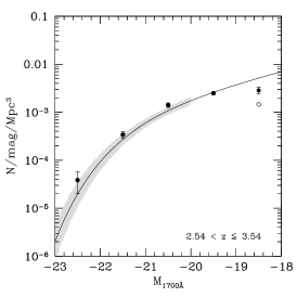
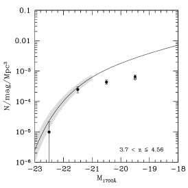
Figure 10: Comparison of the luminosity function at 1700 Å of the FDF with the Schechter function derived in Steidel et al. (1999): $\langle z\rangle\sim 3.04$ (left panel) and $\langle z\rangle\sim 4.13$ (middle panel). The filled (open) symbols show the luminosity function corrected (uncorrected) for $V/V_{max}$. The shaded region in all plots is based only on $\Delta$M^∗, and $\Delta\alpha$ (a detailed discussion concerning the errors $\Delta$M^∗, and $\Delta\alpha$ can be found in Sect. 7), where the cut-off at low luminosity indicates the limiting magnitude of the sample. In the right panel the $1\sigma$ and $2\sigma$ confidence levels for M^∗ and $\alpha$ for a 3 parameter Schechter fit as derived in the FDF in the redshift interval $2.54<z\leq 3.54$ (solid contours) and $3.70<z\leq 4.56$ (dotted contours) are shown. The horizontal dashed line marks the slope $\alpha=-1.6$ as derived in Steidel et al. (1999).

7 Comparison with the literature

In this section we compare the luminosity functions derived in the FDF with the luminosity functions of other surveys. As the cosmology and the wavebands in which the luminosity functions were determined are different from ours for most of the surveys we chose the following approach. First we convert results from the literature to our cosmology ($\Omega_{M}=0.3$, $\Omega_{\Lambda}=0.7$ and $H_{0}=70\,\mathrm{km}\,\mathrm{s}^{-1}\,\mathrm{Mpc}^{-1}$). Note that this conversion may not be perfect, because we can only transform number densities and magnitudes but lack the knowledge of the individual magnitudes and redshifts of the galaxies. Nevertheless, the errors introduced in this way are not large and the method is suitable for our purpose. Second, in order to avoid uncertainties due to conversion between different filter bands, we always use the same band as the survey we want to compare with. Third, we also try to use the same redshift binning if possible. In addition, if the number of galaxies in the FDF is too small to derive a well sampled luminosity function we increase the binning.

To visualize the errors of the literature luminosity functions we perform Monte-Carlo simulations using the $\Delta$M^∗, $\Delta\phi^{\ast}$, and $\Delta\alpha$ given in the papers. In cases where not all of these values could be found in the paper, this is mentioned in the figure caption. We do not take into account any correlation between the Schechter parameters and assume a Gaussian distribution of the errors $\Delta$M^∗, $\Delta\phi^{\ast}$, and $\Delta\alpha$. From 1000 simulated Schechter functions we derive the region where 68.8 % of the realizations lie. The resulting region, roughly corresponding to 1$\sigma$ errors, is shaded in the figures. The luminosity functions derived in the FDF are also shown as filled and open circles. The filled circles are completeness corrected whereas the open circles are not corrected. The redshift binning used to derive the luminosity function in the FDF is given in the lower right part of every figure. Moreover, the limiting magnitude of the respective survey is indicated by the low-luminosity cut-off of the shaded region in all figures. If the limiting magnitude was not explicitly given it was estimated from the figures in the literature.

We first compare our luminosity functions in the UV to the results of Steidel et al. (1999) and the spectroscopic studies of Wilson et al. (2002).

Fig. 10 shows a comparison of the 1700 Å luminosity function derived by Steidel et al. (1999) at redshift $\langle z\rangle\sim 3.04$ (left panel) and $\langle z\rangle\sim 4.13$ (middle panel) with the luminosity function in the FDF. The galaxy sample of Steidel et al. (1999) is based on a R-band ($\langle z\rangle\sim 3.04$) and an I-band ($\langle z\rangle\sim 4.13$) selected catalogue and therefore similar to our I-band selected sample. Candidate galaxies were identified with the Lyman-break technique and most of them spectroscopically confirmed (564 galaxies of the $\langle z\rangle\sim 3.04$ and 46 of the $\langle z\rangle\sim 4.13$ sample, respectively).

To derive the associated errors (shaded region) of the Schechter functions derived by Steidel et al. (1999) we use the errors of M^∗ and $\alpha$ of the $\langle z\rangle\sim 3.04$ sample as given in Fig. 8 of their paper. As there are no errors reported for the $\langle z\rangle\sim 4.13$ sample we assume the same errors as for the $\langle z\rangle\sim 3.04$ sample. Therefore, the shaded region in Fig. 10 (middle panel) is probably a lower limit. For the luminosity function in the FDF we use a redshift binning of $2.54<z\leq 3.54$ (789 galaxies), and $3.70<z\leq 4.56$ (144 galaxies) with the mean redshift of $\langle z\rangle\sim 3.04$ and $\langle z\rangle\sim 4.13$ to be as close as possible to Steidel et al. (1999)’s mean redshifts.

Fig. 10 (left and middle panel) shows that there is very good agreement between the results derived in the FDF and the luminosity function of Steidel et al. (1999) if we focus only on the luminosity function brighter than the limiting magnitudes (shaded regions). On the other hand, because of the depth of the FDF we can trace the luminosity function 2 magnitudes deeper and therefore give better constraints on the slope of the Schechter function. We show in Fig. 10 (right panel) the $1\sigma$ and $2\sigma$ confidence levels for M^∗ and $\alpha$ for a 3 parameter Schechter fit as derived from the FDF in the redshift interval $2.54<z\leq 3.54$ (solid line) and $3.70<z\leq 4.56$ (dotted line). The steep slope $\alpha=-1.6$ derived by Steidel et al. (1999) as marked by the horizontal dashed line can be excluded on a $2\sigma$ level.

Figure 11: Comparison of the luminosity function at 2500 Å of the FDF with the Schechter function derived in Wilson et al. (2002): $0.2<z\leq 0.5$ (left panel), $0.6<z\leq 1.0$ (middle panel), and $1.0<z\leq 1.5$ (right panel). Wilson et al. (2002) fixed the slope to $\alpha=-1.0$ (thick line) and $\alpha=-1.5$ (thin line) and used only M^∗ and $\phi^{\ast}$ as free parameters to determine the Schechter functions.

Wilson et al. (2002) used galaxies selected in the restframe UV with spectroscopic redshifts to derive the luminosity function at 2500 Å in 3 redshift bins: $0.2<z\leq 0.5$ (U’-selected; 403 galaxies), $0.6<z\leq 1.0$ (B-selected; 414 galaxies) and $1.0<z\leq 1.5$ (V-selected; 518 galaxies). As the sample is not deep enough to constrain the slope of the Schechter function Wilson et al. (2002) used two fixed slopes of $\alpha=-1.0$ and $\alpha=-1.5$ to derive the best-fitting Schechter parameters. Since the errors of those parameters are not reported in the paper we can only make qualitative statements about the consistency of their and our luminosity functions: Fig. 11 shows that in the low and intermediate redshift bin there is reasonable agreement with our data, while in contrast to our result, the Schechter functions of Wilson et al. (2002) do not show a significant brightening of $M^{\ast}$ in their highest redshift bin.

Comparison of the FDF luminosity function with the Schechter functions derived in Sullivan et al. (2000), Wolf et al. (2003), Kashikawa et al. (2003), Poli et al. (2001), Iwata et al. (2003), Ouchi et al. (2003b), Blanton et al. (2001), Blanton et al. (2003), and Poli et al. (2003) are presented in Appendix B. In general, we find good agreement at the bright end, where literature datasets are complete. Differences in the faint-end slope in some cases can be attributed to the shallower limiting magnitudes of most of the other surveys.

Figure 12: Comparison of the B-band luminosity function of the FDF with predictions based on Kauffmann et al. (1999)(solid line): $\langle z\rangle\sim 0.20$, $\langle z\rangle\sim 0.62$, $\langle z\rangle\sim 1.05$, $\langle z\rangle\sim 1.46$, $\langle z\rangle\sim 2.12$, and $\langle z\rangle\sim 2.97$ (from upper left to lower right panel). The filled (open) symbols show the luminosity function corrected (uncorrected) for $V/V_{max}$. The drops of the theoretical curves towards the faint-end is caused by the limited mass resolution of the models, see Kauffmann et al. (1999) for details.

8 Comparison with model predictions

As discussed in Sect. 1, key physical processes are involved in shaping the bright and the faint-end of the galaxy luminosity function. Therefore, it is interesting to compare luminosity functions predicted by models with observational results to better constrain those processes. In this section we compare the B-band luminosity function in different redshift bins with model predictions of Kauffmann et al. (1999) and Menci et al. (2002).

Kauffmann et al. (1999):
In Fig. 12 we show the B-band luminosity function of the FDF together with the semi-analytic model predictions by Kauffmann et al. (1999) for the following redshifts: $\langle z\rangle\sim 0.20$, $\langle z\rangle\sim 0.62$, $\langle z\rangle\sim 1.05$, $\langle z\rangle\sim 1.46$, $\langle z\rangle\sim 2.12$, and $\langle z\rangle\sim 2.97$.

There seems to be reasonably good agreement between the models (solid lines) and the luminosity functions derived in the FDF up to redshift $\langle z\rangle\sim 2.12$. Of course at $z\approx 0$ the model is tuned to reproduce the data. At $z\sim 3$, the discrepancy increases as the model does not contain enough bright galaxies. Unfortunately, the models only predict luminosities for massive galaxies and, therefore, they do not predict galaxy number densities below M^∗.

Menci et al. (2002):
In Fig. 13 we compare the B-band luminosity functions of the FDF with the semi-analytic model by Menci et al. (2002) for the following redshifts: $\langle z\rangle\sim 0.3$, $\langle z\rangle\sim 0.6$, $\langle z\rangle\sim 0.9$, $\langle z\rangle\sim 1.4$, $\langle z\rangle\sim 1.9$, $\langle z\rangle\sim 2.6$, $\langle z\rangle\sim 3.4$, and $\langle z\rangle\sim 4.3$.

The agreement between the FDF data and the model in the lowest redshift bin $\langle z\rangle\sim 0.3$ is very good, but this is again expected (see comment above). Moreover, if one focuses the comparison only on the higher luminosity bins considered by Kauffmann et al. (1999), similar acceptable agreement with the data is observed. However, at lower luminosities and higher redshifts, the galaxy density of the simulation is much higher than the observed one.

Figure 13: Comparison of the B-band luminosity function of the FDF with predictions based on the CDM model of Menci et al. (2002) (private communication; solid line): $\langle z\rangle\sim 0.3$, $\langle z\rangle\sim 0.6$, $\langle z\rangle\sim 0.9$, $\langle z\rangle\sim 1.4$, $\langle z\rangle\sim 1.9$, $\langle z\rangle\sim 2.6$, $\langle z\rangle\sim 3.4$, and $\langle z\rangle\sim 4.3$ (from upper left to lower right panel). The filled (open) symbols show the luminosity function corrected (uncorrected) for $V/V_{max}$.

9 Summary and conclusions

We analyzed a sample of about 5600 I-band selected galaxies in the FORS Deep Field down to a limiting magnitude of I $=26.8$ mag.

A comparison with the very deep K-selected catalogue of Labbé et al. (2003) shows, that more than 90 % of their objects are brighter than our limiting I-band magnitude. Therefore our scientific conclusions are not affected by this color bias.

Based on 9 filters we derived accurate photometric redshifts with $\Delta z/(z_{spec}+1)\approx 0.03$ if compared with the spectroscopic sample (Noll et al., 2003; Böhm et al., 2003) of 362 objects. We calculated and presented the luminosity functions in the UV (1500 Å and 2800 Å), u’, B, and g’ bands in the redshift range $0.5<z<5.0$. The error budget of the luminosity functions includes both the photometric redshift error as well as the Poissonian error.

The faint-end slope of the luminosity function does not show a large redshift evolution and is compatible within $2\sigma$ with a constant slope in most of the redshift bins and wavelengths considered here. Furthermore, the slope in the 1500 Å, 2800 Å, and u’ band is very similar but differs from the slope in the g’ and B band. We derive a best fitting slope of $\alpha=-1.07\pm 0.04$ for the combined 1500 Å, 2800 Å and u’ bands and $\alpha=-1.25\pm 0.03$ for the combined g’ and B bands. We find no evidence for a very steep slope ($\alpha\leq-1.6$) at $z\sim 3$ and 1700 Å rest wavelength as reported by other authors (e.g., Steidel et al. 1999, Ouchi et al. 2003b). From our data we can exclude a slope of $\alpha\leq-1.6$ at redshift $\langle z\rangle\sim 3.0$ and $\langle z\rangle\sim 4.0$ at the $2\sigma$ level.

We investigate the evolution of M^∗ and $\phi^{\ast}$ by means of a redshift parameterization of the form $M^{\ast}(z)=M^{\ast}_{0}+a\ln(1+z)$ and $\phi^{\ast}(z)=\phi^{\ast}_{0}(1+z)^{b}$. We find a substantial brightening of M^∗ and a decrease of $\phi^{\ast}$ with redshift in all analyzed wavelengths. If we follow the evolution of the characteristic luminosity from $\langle z\rangle\sim 0.5$ to $\langle z\rangle\sim 5$, we find an increase of $\sim$ 3.1 magnitudes in the UV, of $\sim$ 2.6 magnitudes in the u’ and of $\sim$ 1.6 magnitudes in the g’ and B band. Simultaneously the characteristic density decreases by about 80 % – 90 % in all analyzed wavebands.

Moreover, we compare the luminosity function derived in the FDF with previous observational datasets, mostly based on photometric results, and discuss discrepancies. In general, we find good agreement at the bright end, where their samples are complete. Differences in the faint-end slope in some cases can be attributed to the shallower limiting magnitudes of most of the other surveys. The only observations which reach the same limiting magnitudes as the FDF observations are those of Poli et al. (2001, 2003) and the K-selected sample of Kashikawa et al. (2003). The FDF results for the faint-end slope are in excellent agreement with those of Kashikawa et al. (2003) but the slope of the Schechter function favored by Poli et al. (2001, 2003) is steeper than we would expect from the FDF.

The semi-analytical models predict luminosity functions which describe (by construction) the data at low redshift quite well, but show growing disagreement with increasing redshifts.

Appendix A Schechter parameters

Figure 14: Luminosity functions at 1500 Å from low redshift ($\langle z\rangle=0.3$, upper left panel) to high redshift ($\langle z\rangle=5.5$, lower right panel). The filled (open) symbols show the luminosity function corrected (uncorrected) for $V/V_{max}$. The fitted Schechter functions for a fixed slope $\alpha$ are shown as solid lines. Note that we only fit the luminosity functions from $\langle z\rangle=0.6$ to $\langle z\rangle=4.5$. The parameters of the Schechter functions can be found in Table 5. The Schechter fit for redshift $\langle z\rangle=0.6$ is indicated as dashed line in all panels.

Table 5: Schechter function fit at 1500 Å

redshift interval	M∗ (mag)	$\phi^{\ast}$ (Mpc-3)	$\alpha$ (fixed)
0.45 – 0.81	$-$18.17 +0.11 $-$0.11	0.0110 +0.0007 $-$0.0006	$-$1.07
0.81 – 1.11	$-$18.85 +0.10 $-$0.10	0.0103 +0.0006 $-$0.0006	$-$1.07
1.11 – 1.61	$-$19.48 +0.11 $-$0.11	0.0056 +0.0006 $-$0.0005	$-$1.07
1.61 – 2.15	$-$19.97 +0.22 $-$0.24	0.0033 +0.0006 $-$0.0006	$-$1.07
2.15 – 2.91	$-$20.61 +0.09 $-$0.09	0.0032 +0.0002 $-$0.0002	$-$1.07
2.91 – 4.01	$-$20.72 +0.09 $-$0.10	0.0023 +0.0002 $-$0.0002	$-$1.07
4.01 – 5.01	$-$21.00 +0.15 $-$0.11	0.0010 +0.0001 $-$0.0001	$-$1.07

Table 6: Schechter function fit at 2800 Å

redshift interval	M∗ (mag)	$\phi^{\ast}$ (Mpc-3)	$\alpha$ (fixed)
0.45 – 0.81	$-$18.80 +0.15 $-$0.15	0.0104 +0.0007 $-$0.0007	$-$1.07
0.81 – 1.11	$-$19.52 +0.09 $-$0.10	0.0089 +0.0005 $-$0.0005	$-$1.07
1.11 – 1.61	$-$20.03 +0.09 $-$0.09	0.0053 +0.0004 $-$0.0004	$-$1.07
1.61 – 2.15	$-$20.43 +0.18 $-$0.17	0.0029 +0.0005 $-$0.0004	$-$1.07
2.15 – 2.91	$-$21.16 +0.09 $-$0.08	0.0030 +0.0002 $-$0.0002	$-$1.07
2.91 – 4.01	$-$21.19 +0.10 $-$0.08	0.0021 +0.0002 $-$0.0001	$-$1.07
4.01 – 5.01	$-$21.55 +0.17 $-$0.21	0.0009 +0.0001 $-$0.0001	$-$1.07

Figure 15: Luminosity functions in the u’-band from low redshift ($\langle z\rangle=0.3$, upper left panel) to high redshift ($\langle z\rangle=5.5$, lower right panel). The filled (open) symbols show the luminosity function corrected (uncorrected) for $V/V_{max}$. The fitted Schechter functions for a fixed slope $\alpha$ are shown as solid lines. Note that we only fit the luminosity functions from $\langle z\rangle=0.6$ to $\langle z\rangle=4.5$. The parameters of the Schechter functions can be found in Table 7. The dotted line represents the local u’-band luminosity function derived from the SDSS (Blanton et al., 2001). The Schechter fit for redshift $\langle z\rangle=0.6$ is indicated as dashed line in all panels.

Table 7: Schechter function fit in the u’-band

redshift interval	M∗ (mag)	$\phi^{\ast}$ (Mpc-3)	$\alpha$ (fixed)
0.45 – 0.81	$-$19.56 +0.16 $-$0.15	0.0096 +0.0006 $-$0.0006	$-$1.07
0.81 – 1.11	$-$20.12 +0.10 $-$0.10	0.0080 +0.0004 $-$0.0004	$-$1.07
1.11 – 1.61	$-$20.56 +0.08 $-$0.09	0.0049 +0.0003 $-$0.0003	$-$1.07
1.61 – 2.15	$-$20.70 +0.18 $-$0.16	0.0033 +0.0004 $-$0.0004	$-$1.07
2.15 – 2.91	$-$21.50 +0.08 $-$0.08	0.0032 +0.0002 $-$0.0002	$-$1.07
2.91 – 4.01	$-$21.57 +0.11 $-$0.10	0.0022 +0.0002 $-$0.0002	$-$1.07
4.01 – 5.01	$-$21.92 +0.24 $-$0.20	0.0008 +0.0002 $-$0.0001	$-$1.07

Table 8: Schechter function fit in the g’-band

redshift interval	M∗ (mag)	$\phi^{\ast}$ (Mpc-3)	$\alpha$ (fixed)
0.45 – 0.81	$-$21.47 +0.20 $-$0.20	0.0042 +0.0003 $-$0.0003	$-$1.25
0.81 – 1.11	$-$21.72 +0.15 $-$0.15	0.0039 +0.0003 $-$0.0003	$-$1.25
1.11 – 1.61	$-$22.01 +0.14 $-$0.14	0.0026 +0.0002 $-$0.0002	$-$1.25
1.61 – 2.15	$-$21.82 +0.20 $-$0.20	0.0020 +0.0004 $-$0.0003	$-$1.25
2.15 – 2.91	$-$22.62 +0.13 $-$0.10	0.0020 +0.0002 $-$0.0002	$-$1.25
2.91 – 4.01	$-$22.51 +0.13 $-$0.14	0.0016 +0.0002 $-$0.0002	$-$1.25
4.01 – 5.01	$-$23.12 +0.22 $-$0.23	0.0005 +0.0001 $-$0.0001	$-$1.25

Figure 16: Luminosity functions in the B-band from low redshift ($\langle z\rangle=0.3$, upper left panel) to high redshift ($\langle z\rangle=5.5$, lower right panel). The filled (open) symbols show the luminosity function corrected (uncorrected) for $V/V_{max}$. The fitted Schechter functions for a fixed slope $\alpha$ are shown as solid lines. Note that we only fit the luminosity functions from $\langle z\rangle=0.6$ to $\langle z\rangle=4.5$. The parameters of the Schechter functions can be found in Table 9. The Schechter fit for redshift $\langle z\rangle=0.6$ is indicated as dashed line in all panels.

Table 9: Schechter function fit in the B-band

redshift interval	M∗ (mag)	$\phi^{\ast}$ (Mpc-3)	$\alpha$ (fixed)
0.45 – 0.81	$-$21.28 +0.21 $-$0.18	0.0042 +0.0004 $-$0.0003	$-$1.25
0.81 – 1.11	$-$21.57 +0.15 $-$0.13	0.0040 +0.0003 $-$0.0002	$-$1.25
1.11 – 1.61	$-$21.91 +0.13 $-$0.13	0.0024 +0.0002 $-$0.0002	$-$1.25
1.61 – 2.15	$-$21.65 +0.22 $-$0.22	0.0021 +0.0004 $-$0.0004	$-$1.25
2.15 – 2.91	$-$22.44 +0.11 $-$0.09	0.0021 +0.0002 $-$0.0002	$-$1.25
2.91 – 4.01	$-$22.44 +0.15 $-$0.14	0.0015 +0.0002 $-$0.0002	$-$1.25
4.01 – 5.01	$-$22.81 +0.21 $-$0.25	0.0005 +0.0001 $-$0.0001	$-$1.25

Appendix B Comparison with literature

In this appendix we compare the luminosity functions derived in the FDF with the results of further publications as introduced in Sect. 7. The filled (open) circles show the completeness corrected (uncorrected) luminosity function as derived in the FDF in the redshift bin listed in the lower right corner. The solid line(s) represent the Schechter function given in the different papers transformed to our cosmology. To visualize the errors associated to this Schechter function we perform a Monte-Carlo simulation using the errors of the Schechter parameters reported in the specific paper (see Sect. 7 for more details). As the errors for all three Schechter parameters ($\Delta$M^∗, $\Delta\phi^{\ast}$, and $\Delta\alpha$) are not always given in the paper, we denote in the caption the errors used to perform the simulation. The region wherein 68.8 % of the realizations lie are shown as shaded region in the plots and corresponds roughly to the 1$\sigma$ error due to the Schechter errors reported in the figure captions. Moreover the cut-off of the shaded region marks the limiting magnitude of the survey we compare with.

B.1 UV bands

Sullivan et al. (2000):
Although the volume of the FDF at low redshift is rather small, and therefore is not well suited to properly sample the bright end of the Schechter function, we compare for completeness in Fig. 17 our luminosity function also with the luminosity function derived in Sullivan et al. (2000). Their sample contains 433 UV-selected sources within an area of $2.2deg^{2}$. 273 of these objects are galaxies and cover the redshift range $z\simeq 0-0.4$. The solid line in Fig. 17 represents the luminosity function at 2000 Å from Sullivan et al. (2000) whereas the filled circles shows our $V/V_{max}$ corrected luminosity function derived at $0.15<z\leq 0.4$. Despite the small volume, the I-selected catalogue and the extrapolated 2000 Å luminosity function (see above) there is a general agreement with only small systematic offsets (probably also due to a known cluster at $z\sim 0.33$ (Noll et al., 2003)). This is an additional confirmation of the validity of our technique to derive the luminosity function as described in Sect. 5.1.

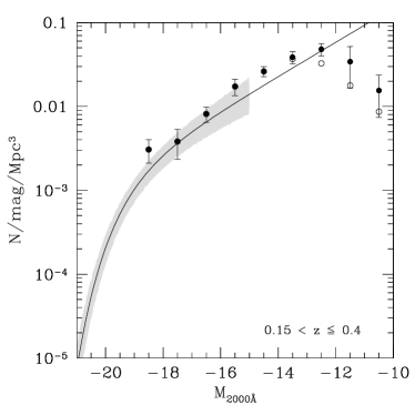
Figure 17: Comparison of the luminosity function at 2000 Å of the FDF with the Schechter function derived in Sullivan et al. (2000) ($z\simeq 0-0.4$). The shaded region is based on $\Delta$M^∗, $\Delta\phi^{\ast}$, and $\Delta\alpha$, where the cut-off at low luminosity indicates the limiting magnitude of the sample.

Wolf et al. (2003):
In Fig. 18 we compare the luminosity function at 2800 Å of the FDF with the R-band selected luminosity function derived in the COMBO-17 survey (Wolf et al., 2003) for different redshift bins: 0.2 – 0.6, 0.6 – 0.8, 0.8 – 1.0, 1.0 – 1.2. Because of the limited sample size of the FDF at low redshift we could not use the same local redshift binning as Wolf et al. (2003). We compare therefore in Fig. 18 (upper left panel) the COMBO17 Schechter function at $\langle z\rangle\sim 0.3$ (light gray) and $\langle z\rangle\sim 0.5$ (dark gray) with the FDF luminosity function derived at $0.2<z\leq 0.6$. There is an overall good agreement between the FDF data and the COMBO-17 survey at all redshifts under investigations if we compare only the magnitude range in common to both surveys (shaded region). Nevertheless the number density of the FDF seems to be slightly higher which most probably can be attributed to cosmic variance. The Wolf et al. (2003) team derived the faint-end slope from relatively shallow data which have only a limited sensitivity for the faint-end slope. Thus, the disagreement between the much deeper FDF data and the Wolf et al. (2003) results at $z\sim 0.5$ and for $z>1$ does not come as a surprise.

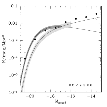
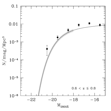
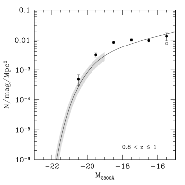
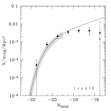
Figure 18: Comparison of the luminosity function at 2800 Å of the FDF with the Schechter function derived in Wolf et al. (2003): $0.2<z\leq 0.4$ (upper left panel, light gray), $0.4<z\leq 0.6$ (upper left panel, dark grey), $0.6<z\leq 0.8$ (upper right panel), $0.8<z\leq 1.0$ (lower left panel), $1.0<z\leq 1.2$ (lower right panel). The shaded regions of all plots are based on $\Delta$M^∗, $\Delta\phi^{\ast}$, and $\Delta\alpha$, where the cut-off at low luminosity indicates the limiting magnitude of the sample.

Kashikawa et al. (2003):
In Fig. 19 we compare our luminosity function with the K-band selected 2000 Å luminosity function of Kashikawa et al. (2003) derived in the Subaru Deep Survey. They used photometric redshift to determine the distance for 439 field galaxies. There is a good overall agreement of the luminosity functions in the redshift bins $0.6<z\leq 1.0$, $1.0<z\leq 1.5$, $1.5<z\leq 2.5$. Only in the highest redshift bin ($2.5<z\leq 3.5$) the number density derived in Kashikawa et al. (2003) is lower by a factor of about 2 when compared with the FDF.

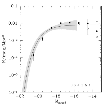
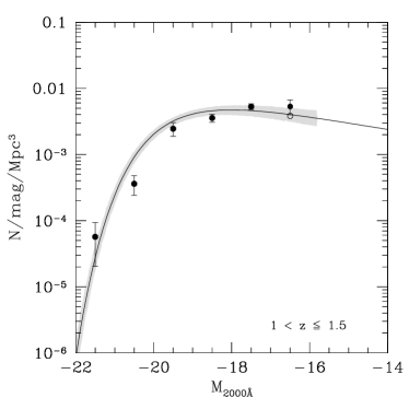
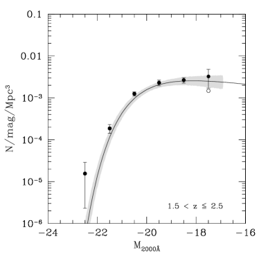
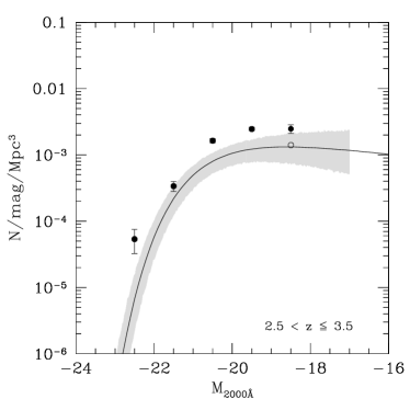
Figure 19: Comparison of the luminosity function at 2000 Å of the FDF with the Schechter function derived in Kashikawa et al. (2003): $0.6<z\leq 1.0$ (upper left panel), $1.0<z\leq 1.5$ (upper right panel), $1.5<z\leq 2.5$ (lower left panel), $2.5<z\leq 3.5$ (lower right panel). The shaded regions of all plots are based on $\Delta$M^∗, $\Delta\phi^{\ast}$, and $\Delta\alpha$, where the cut-off at low luminosity indicates the limiting magnitude of the sample.

Poli et al. (2001):
Poli et al. (2001) combined three pencil beam surveys as the HDFN, the HDFS and the New Technology Telescope Deep Field (Arnouts et al., 1999) reducing the influence of cosmic variance and derived the 1700 Å luminosity function at $2.5<z\leq 3.5$. In Fig. 20 we compare the result with the luminosity function in the FDF. There is very good agreement although the slope of the Schechter function ($\alpha=-1.37$) is slightly steeper than we would expect from the FDF.

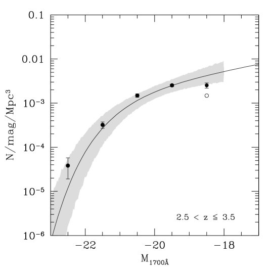
Figure 20: Comparison of the luminosity function at 1700 Å of the FDF with the Schechter function derived in Poli et al. (2001) ($2.50<z\leq 3.50$ ). The shaded region is based only on $\Delta$M^∗, and $\Delta\alpha$, where the cut-off at low luminosity indicates the limiting magnitude of the sample.

Iwata et al. (2003):
Iwata et al. (2003) analyzed about 300 galaxies in a 575 square-arcmin field detected in the I and z band at redshift $z\sim 5$, selected by means of the Lyman-break technique. They derived the luminosity function at 1700 Å statistically. We analize Table 3 of Iwata et al. (2003) with the same method as described in Sect. 5.1 to get approximate errors for M^∗ and $\phi^{\ast}$ for a fixed slope of $\alpha=-1.5$ (as given in the paper). From these $\Delta$M^∗ and $\Delta\phi^{\ast}$ we calculate the shaded region of Fig. 21 (left panel). Fig. 21 (left panel) compares the luminosity function of Iwata et al. (2003) with the luminosity function of the FDF derived at $4.01<z\leq 5.01$. Although the number density of Iwata et al. (2003) at $z\sim 5$ seems to be slightly lower than the number density derived in the FDF at $\langle z\rangle\sim 4.5$ the overall agreement is rather good. On the other hand, part of this decrease in density may also be due to intrinsic evolution between redshift $\langle z\rangle\sim 4.5$ and $\langle z\rangle\sim 5.0$. According to our evolution model as derived in Sect. 6 we would expect a decrease of $\phi^{\ast}$ of about 15 %.

Ouchi et al. (2003b):
Ouchi et al. (2003b) investigated photometric properties of about 2600 Lyman-break galaxies at $z=3.5-5.2$. Based on this sample they derived the luminosity function at 1700 Å for three redshift bins: $z=4.0\pm 0.5$, $z=4.7\pm 0.5$, $z=4.9\pm 0.3$. In Fig. 21 (right panel) we compare their Schechter function for a fixed slope of $\alpha=-1.6$ with the luminosity function of the FDF derived at $4.01<z\leq 5.01$. The Schechter function for $z=4.0\pm 0.5$ is shaded in dark gray, the $z=4.7\pm 0.5$ Schechter Function is shaded light gray and the $z=4.9\pm 0.3$ Schechter Function is represented by the dashed line (no errors reported). It is difficult to compare the results of Ouchi et al. (2003b) with the FDF. Our data favor a less steep slope of the luminosity function than advocated by Ouchi et al. (2003b).

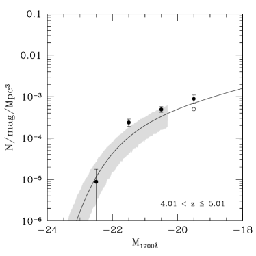
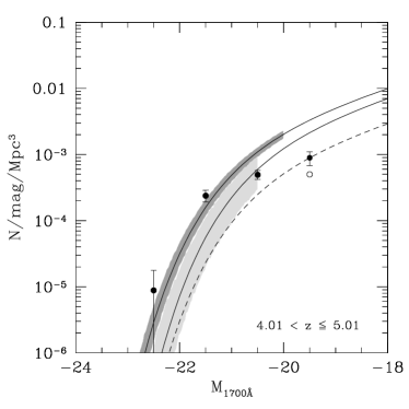
Figure 21: Left panel: Comparison of the luminosity function at 1700 Å of the FDF with the Schechter function derived in Iwata et al. (2003) ($z\sim 5$). The shaded region is based only on $\Delta$M^∗, and $\Delta\phi^{\ast}$. Right panel: Comparison of the luminosity function at 1700 Å of the FDF with the Schechter functions derived in Ouchi et al. (2003b): $z=4.0\pm 0.5$ (dark shaded), $z=4.7\pm 0.5$ (light shaded), and $z=4.9\pm 0.3$ (not shaded; dashed line). Both shaded regions are based only on $\Delta$M^∗, and $\Delta\phi^{\ast}$, where the cut-off at low luminosity indicates the limiting magnitude of the sample.

B.2 SDSS bands (u’, g’, ^0.1u, ^0.1g)

In this section we want to compare the luminosity function in the FDF with the one from the SDSS.

In Fig.  22 (left panel) and Fig. 23 (left panel) we show the luminosity function derived in Blanton et al. (2001) for $z\sim 0.1$ in the u’ and g’ band, respectively, as light shaded region. To make a more appropriate comparison between our ‘local’ results derived at $0.15<z\leq 0.45$, we evolve the Schechter function of Blanton et al. (2001) to $\langle z\rangle\sim 0.3$ according to our evolutionary model described in Sect. 6. We use for the u’-band the parameter $a=-1.80$ and $b=-1.70$ whereas for the g’-band we use $a=-1.08$ and $b=-1.29$. The evolved Schechter function is shown as dark shaded region in in Fig. 22 (left panel) and Fig. 23 (left panel) for the u’ and g’ band, respectively. Despite the small volume of the FDF in the local redshift bin, the agreement is very good in both bands and especially in the g’-band. We therefore conclude that there is no hint of a possible systematic offset between the two datasets.

In Fig. 22 (right panel) and Fig. 23 (right panel) we also show the luminosity function derived in Blanton et al. (2003) for the blue-shifted filter ^0.1u and ^0.1g. Again, the light shaded region represents the $\langle z\rangle\sim 0.1$ luminosity function whereas the dark shaded region shows the luminosity function evolved to $\langle z\rangle\sim 0.3$. We use the same evolution parameter as derived for u’ and g’. The approach used by Blanton et al. (2003) differs from those used in all other studies, including ours and the previous SDSS (Blanton et al., 2001) results. It is therefore beyond the scope of the paper to explain the discrepancies.

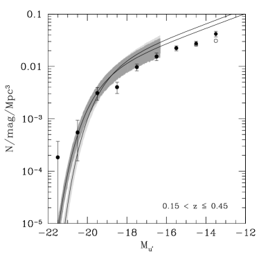
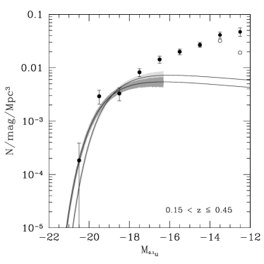
Figure 22: Left panel: Comparison of the u’-band luminosity function of the FDF with the Schechter function derived in Blanton et al. (2001) at $z\sim 0.1$ (light shaded). The dark shaded region shows the Schechter function of Blanton et al. (2001) evolved according to our evolutionary model described in Sect. 6 to redshift $z\sim 0.3$. The shaded regions are based on $\Delta$M^∗, $\Delta\phi^{\ast}$, and $\Delta\alpha$. Right panel: Comparison of the ^0.1u-band luminosity function of the FDF with the Schechter function derived in Blanton et al. (2003) at $z\sim 0.1$ (light shaded). The dark shaded region shows the Schechter function of Blanton et al. (2003) evolved according to our evolutionary model described in Sect. 6 to redshift $z\sim 0.3$. The shaded regions are based on $\Delta$M^∗, $\Delta\phi^{\ast}$, and $\Delta\alpha$, where the cut-off at low luminosity indicates the limiting magnitude of the sample.

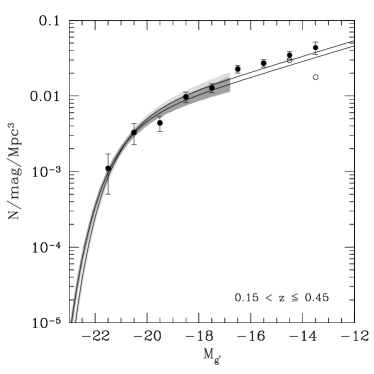
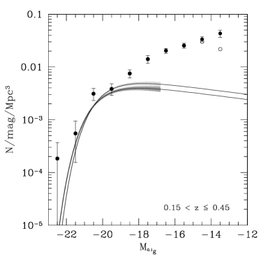
Figure 23: Left panel: Comparison of the g’-band luminosity function of the FDF with the Schechter function derived in Blanton et al. (2001) at $z\sim 0.1$ (light shaded). The dark shaded region shows the Schechter function of Blanton et al. (2001) evolved according to our evolutionary model described in Sect. 6 to redshift $z\sim 0.3$. The shaded regions are based on $\Delta$M^∗, $\Delta\phi^{\ast}$, and $\Delta\alpha$. Right panel: Comparison of the ^0.1g-band luminosity function of the FDF with the Schechter function derived in Blanton et al. (2003) at $z\sim 0.1$ (light shaded). The dark shaded region shows the Schechter function of Blanton et al. (2003) evolved according to our evolutionary model described in Sect. 6 to redshift $z\sim 0.3$. The shaded regions are based on $\Delta$M^∗, $\Delta\phi^{\ast}$, and $\Delta\alpha$, where the cut-off at low luminosity indicates the limiting magnitude of the sample.

B.3 B-band

Poli et al. (2003):
Poli et al. (2003) analyzed 1541 I-selected and 138 K-selected galaxies to construct the B-band luminosity function up to redshift $\langle z\rangle\sim 3$. A comparison between the luminosity function of Poli et al. (2003) and the FDF is shown in Fig. 24 for the redshift bins $0.4<z\leq 0.7$ (upper left panel), $0.7<z\leq 1.0$ (upper right panel), $1.3<z\leq 2.5$ (lower left panel) and $2.5<z\leq 3.5$ (lower right panel).

In neither of the redshift bins an error for $\phi^{\ast}$ is reported in the paper and therfore could not be included in the simulation of the shaded region. For the two lower redshift bins ($0.4<z\leq 0.7$ and $0.7<z\leq 1.0$) the shaded region is based on $\Delta$M^∗ and $\Delta\phi^{\ast}$ whereas in the high redshift bins ($1.3<z\leq 2.5$ and $2.5<z\leq 3.5$) the shown error of the Schechter function (shaded region) is based only on $\Delta$M^∗. If this is taken into account, the results of Poli et al. (2003) are in good agreement with the FDF, but again, the slope of the Schechter function is too steep when compared with the FDF luminosity function. On the other hand the brightening of M^∗ with redshift is present in both samples.

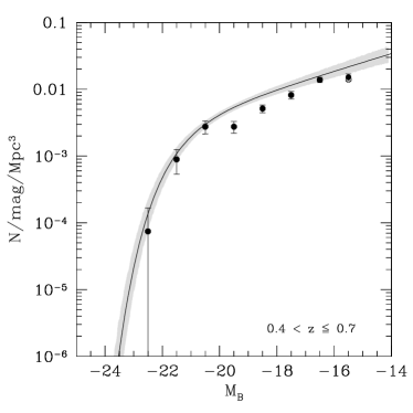
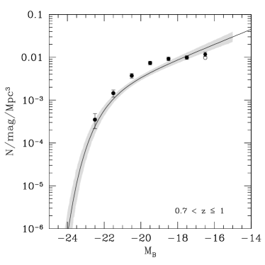
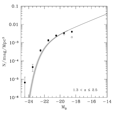
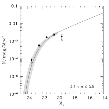
Figure 24: Comparison of the B-band luminosity function of the FDF with the Schechter function derived in Poli et al. (2003): $0.4<z\leq 0.7$ (upper left panel), $0.7<z\leq 1.0$ (upper right panel), $1.3<z\leq 2.5$ (lower left panel), and $2.5<z\leq 3.5$ (lower right panel). The shaded region is based only on $\Delta$M^∗, and $\Delta\alpha$ for $0.4<z\leq 0.7$, and $0.7<z\leq 1.0$, whereas for the $1.3<z\leq 2.5$, and $1.3<z\leq 2.5$ the shaded region is based only on $\Delta$M^∗, where the cut-off at low luminosity indicates the limiting magnitude of the sample.

Appendix C Confidence levels for the slope

Figure 25: $1\sigma$ and $2\sigma$ confidence levels in Schechter parameter space. A Schechter function with three free parameters M^∗, $\phi^{\ast}$, and $\alpha$ has been fitted to the luminosity function at 1500 Å (upper left panel), 2800 Å (upper right panel), u’ (lower left panel) and g’-band (lower right panel) and projected to the M^∗ – $\alpha$ plane. The various contours in each panel correspond to the different redshift bins, ranging from $\langle z\rangle=0.6$ (low luminosity) to $\langle z\rangle=3.5$ (high luminosity). We alternate continuous and dotted lines for clarity. The dashed line marks the fixed slope ($\alpha(z)=\mathrm{const.}$) used to derive the luminosity functions in the different wavebands (see Table 3 lower part).