An XMM-Newton observation of the massive, relaxed galaxy cluster ClJ1226.9$+$3332 at $z=0.89$

Abstract

A detailed X-ray analysis of an XMM-Newton observation of the high-redshift (z=0.89) galaxy cluster ClJ1226.9$+$3332 is presented. After careful consideration of background subtraction issues, the X-ray temperature is found to be $11.5^{+1.1}_{-0.9}\mbox{$\mathrm{~{}keV}$}$, the highest X-ray temperature of any cluster at $z>0.6$. The temperature is consistent with the observed velocity dispersion. In contrast to MS1054-0321, the only other very hot cluster currently known at $z>0.8$, ClJ1226.9$+$3332 features a relaxed X-ray morphology, and its high overall gas temperature is not caused by one or several hot spots. The system thus constitutes a unique example of a high redshift (z$>$0.8), high temperature (T$>$10 keV), relaxed cluster, for which the usual hydrostatic equilibrium assumption, and the X-ray mass is most reliable.

A temperature profile is constructed (for the first time at this redshift) and is consistent with the cluster being isothermal out to $45\%$ of the virial radius. Within the virial radius (corresponding to a measured overdensity of a factor of 200), a total mass of $1.4\pm 0.5\times 10^{15}M_{\odot}$ is derived, with a gas mass fraction of $12\pm 5\%$ (for a $\Lambda$CDM cosmology and H₀=70 km s^-1 Mpc^-1). This total mass is similar to that of the Coma cluster. The bolometric X-ray luminosity is $5.3^{+0.2}_{-0.2}\times 10^{45}\mathrm{\mbox{$\mathrm{~{}erg}$}\mathrm{\mbox{$\mathrm{~{}s}$}^{-1}}}$. Analysis of a short Chandra observation confirms the lack of significant point-source contamination, the temperature, and the luminosity, albeit with lower precision. The probabilities of finding a cluster of this mass within the volume of the discovery X-ray survey are $\sim 8\times 10^{-5}$ for $\Omega_{M}=1$ and $0.64$ for $\Omega_{M}=0.3$, making $\Omega_{M}=1$ highly unlikely.

The entropy profile suggests that entropy evolution is being observed. The metal abundance (of $Z=0.33^{+0.14}_{-0.10}\mathrm{Z_{\odot}}$), gas mass fraction, and gas distribution are consistent with those of local clusters; thus the bulk of the metals were in place by z=0.89.

1 Introduction

Massive galaxy clusters form from the high-sigma tail of the initial cosmological density distribution. As a result they are rare, but also very powerful probes of cosmology. Given an assumed initial density distribution, the properties of the massive cluster population can be predicted under alternate cosmologies, and those predictions tested with observations. The predictions of different cosmologies diverge with redshift, making high-redshift, massive clusters the most useful objects to distinguish between them.

X-ray observations of galaxy clusters provide a useful means of measuring their properties. The intra-cluster gas is extremely luminous in X-rays, and measurements of the gas temperature and density distributions allow the total mass of the system (the property most directly related to cosmological predictions) to be inferred. This inference requires, however, that the intra-cluster medium (ICM) be in hydrostatic equilibrium. If, as believed, clusters form through a series of hierarchical mergers, then this will only be the case some time after the last merger. Thus the most useful objects to study for the purpose of constraining cosmological models in this way, are high-redshift, massive, relaxed clusters of galaxies. These are extremely rare.

However the question of when a cluster can be considered to be relaxed is something of a contentious issue. In a study of $368$ low$-z$ clusters observed by Einstein , Jones & Forman (1999) found $\approx 40\%$ to have substructure in their X-ray images. This fraction is likely to be an underestimate, as Einstein was unable to resolve small scale substructure. More recently, the high resolving power of Chandra has revealed substructure in clusters that were previously considered to be relaxed, such as A1795 (Fabian et al., 2001; Markevitch et al., 2001), and MS 1455.0+2232 (Mazzotta et al., 2002). On the other hand, X-ray derived masses of clusters that appear relaxed in Chandra observations have been found to agree well with independent weak lensing mass measurements, at least in the inner regions (Allen et al., 2001, and references therein).

While Chandra can accurately probe the gas properties in the central regions of clusters, the strength of XMM-Newton lies in its large collecting area, which allows it to trace the gas density and temperature structure out into the low surface-brightness emission at large radii, even at high redshifts. This minimises the uncertainties involved in extrapolating these properties out to the virial radius when deriving the total mass of the system. The mass composition of massive galaxy clusters (e.g. the baryonic to total mass fraction) is believed to be representative of the universe as a whole, due to their large size (e.g. Allen et al., 2002). Thus by directly observing the ICM out to large radii, one obtains a more representative measurement of these properties.

In June 2001, XMM-Newton made a $30\mbox{$\mathrm{~{}ks}$}$ observation of galaxy cluster ClJ1226.9$+$3332, one of the most distant, luminous clusters found in the WARPS X-ray selected survey (Scharf et al., 1997; Jones et al., 1998; Ebeling et al., 2000; Perlman et al., 2002). The cluster was positioned $\approx 4\mathrm{{}^{\prime}}$ off-axis in order to investigate other candidate clusters in the field, to be described in a future paper. The discovery ROSAT data indicated a high X-ray luminosity, but were insufficient to accurately determine morphology or temperature. Optical follow up found the cluster’s redshift to be $0.89$ (Ebeling et al., 2001), corresponding to a look back time of over half of the age of the universe, and Sunyaev-Zel’dovich effect imaging confirmed that the cluster is both hot and massive (Joy et al., 2001). We present here the results of a detailed analysis of the XMM-Newton data. There is also a fairly short ($10\mbox{$\mathrm{~{}ks}$}$) archived Chandra observation of ClJ1226.9$+$3332, which has been examined by Cagnoni et al. (2001). We have analysed these data in a way consistent with our XMM-Newton analysis in order to check consistency, and we draw comparisons at several relevant points.

Throughout this paper, a cosmology of $H_{0}=70\mathrm{\mbox{$\mathrm{~{}km}$}\mathrm{\mbox{$\mathrm{~{}s}$}^{-1}}\mathrm{\mbox{$\mathrm{~{}Mpc}$}^{-1}}\,}$, and $\Omega_{M}=0.3$ ($\Omega_{\Lambda}=0.7$) is adopted, unless stated otherwise, and all errors are quoted at the $68\%$ level. At the cluster’s redshift, $1\mathrm{{}^{\prime}}\hskip-1.00006pt\mathrm{{}^{\prime}}$ corresponds to $7.8\mbox{$\mathrm{~{}kpc}$}$ in this cosmology. The virial radius ($r_{\mathrm{200}}$) is defined as the radius within which the mean density is $200$ times the critical density at the redshift of observation.

2 Data Preparation

The data from the PN and two MOS detectors were processed with the processing chains, epchain (PN) and emchain (MOS) as these have been found to be significantly better at removing bad events and pixels than the standard ‘procs’ (epproc and emproc). Examination of the processed PN events showed that a few bad pixels (two rows, and one pixel) were undetected by the chain, and these were added to the bad pixel tables, and the data was reprocessed. Lightcurves of the three detectors, produced in the $10-15\mbox{$\mathrm{~{}keV}$}$ band showed that the observation was contaminated by several large background flares. The periods of very high background were selected by eye, and removed from the lightcurve, before the remaining data were cleaned by a recursive $3-\sigma$ clipping algorithm to leave a stable mean rate. The lightcurve of the PN detector is shown in Fig. 1, with the accepted times indicated by the bar underneath the lightcurve.

Figure 1: Lightcurve of the pn observation of ClJ1226.9$+$3332, in $50\mbox{$\mathrm{~{}s}$}$ bins in the range $10-15\mbox{$\mathrm{~{}keV}$}$. The bar below the lightcurve indicates the good time intervals left after cleaning, and the dashed line indicates the $3\sigma$ cut-off level (see text).

Events were filtered on the basis of their pattern parameter, which indicates the geometry of the detection of each event, i.e. the number of adjacent pixels that detect each photon. Events whose patterns are considered well calibrated (PN - single and double, MOS - single, double, and quadruple) were retained in the filtering.

In the analysis of XMM-Newton data, one must carefully account for the background contamination. There are, broadly speaking, two ways of doing this; one may sample the background locally, from the same observation as the source, or one may use a ‘blank-sky’ background dataset, composed of many observations, with all bright sources removed (Lumb et al., 2002).

The background is composed of three types of events:

• Soft protons - this component is believed to be caused by solar flares, and the intensity and spectrum of this component varies significantly with time. It is the dominant component during flaring intervals, but in quiescent periods its contribution is the smallest. This component is vignetted, but may not have the same vignetting function as the X-rays.

• X-rays - this component dominates the background at low energies ($<1.5\mbox{$\mathrm{~{}keV}$}$), and varies spatially across the sky (though not significantly across the field-of-view). This component is vignetted by the telescopes.

• Cosmic-ray induced particles - this component dominates at high energies, and is induced by high energy cosmic rays passing unvignetted through the instrument. This component is referred to hereafter as the particle background.

This observation of ClJ1226.9$+$3332 appears to be contaminated by a particularly high background level, even after lightcurve cleaning. As shown in Fig. 1, there are two intervals of lower background separated by a large flaring event. During the first interval ($2-11\mbox{$\mathrm{~{}ks}$}$), for the PN camera, the average count rate ($10-15\mbox{$\mathrm{~{}keV}$}$) was $1.81\mathrm{~{}counts\mathrm{\mbox{$\mathrm{~{}s}$}^{-1}}}$, while in the second($18-26\mbox{$\mathrm{~{}ks}$}$), the mean rate was $0.97\mathrm{~{}counts\mathrm{\mbox{$\mathrm{~{}s}$}^{-1}}}$. For comparison, the PN count rate in the blank-sky datasets in this energy band was $0.52\mathrm{~{}counts\mathrm{\mbox{$\mathrm{~{}s}$}^{-1}}}$. Even considering the $10-20\%$ variations in the background level found by Lumb et al. (2002), the background in these two periods is higher than would normally be acceptable. The count rates outside the field of view, which consist only of particle events, were also compared. The count rate was a factor of $1.7$ higher in the ClJ1226.9$+$3332 dataset than the blank-sky data. This shows that the high background level in this dataset is due to high levels of both particles and soft protons. This significantly increases the difficulty and uncertainties involved with using a blank-sky background in the analysis.

Due to the high background, a careful comparison of spectral analysis methods was made (using both local and blank-sky backgrounds), on both of the time periods separately, and combined (for simplicity, hereafter, the first period ($2-11\mbox{$\mathrm{~{}ks}$}$) will be referred to as the “high background period”, and the second ($18-26\mbox{$\mathrm{~{}ks}$}$) will be referred to as the “low background period”). This analysis is described in some detail in the following sections, but the general conclusion was that in the low background period, all methods gave consistent results, and that if a local background was used, then the results from the high background and low background periods, and both periods combined were consistent. As discussed in §4.6 our final results are taken from the combined periods with a local background, which contained a useful time of $14\mbox{$\mathrm{~{}ks}$}$ for the PN detector, and $18\mbox{$\mathrm{~{}ks}$}$ for each of the two MOS detectors.

The Chandra observation was performed with the ACIS-S array exposed, with the target on the S3 chip. Only standard data preparation was required, as there were no significant background flares during the short exposure.

3 Imaging analysis

A combined, exposure-corrected image of the datasets of the PN and two MOS cameras in the energy band $0.3-8\mbox{$\mathrm{~{}keV}$}$ was produced, and adaptively smoothed. Contours of this smoothed emission are shown in Fig. 2, overlaid on an optical image. The outer contours are reasonably circular, suggesting the X-ray emitting gas is fairly relaxed. The lowest contour, at a level of $0.45\mathrm{~{}counts~{}pixel^{-1}}$ (which is $1.5$ times the background level) is distorted due to the point source in the West, and truncated slightly along the South-East edge due to a PN CCD gap that was not fully removed by the exposure correction.

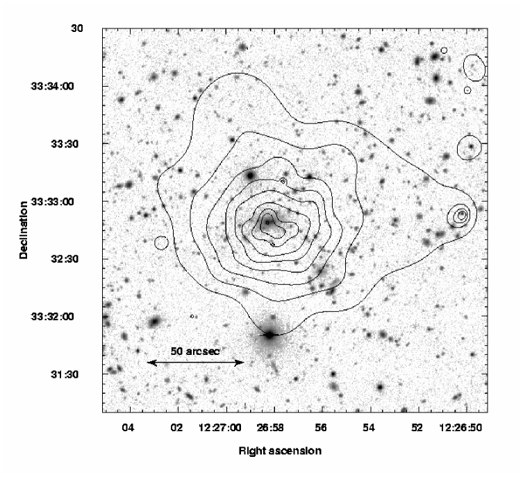
Figure 2: Contours of X-ray emission detected by XMM-Newton $0.3-8\mbox{$\mathrm{~{}keV}$}$ overlaid on a Subaru I-Band image of cluster ClJ1226.9$+$3332. The contours were taken of data from the three cameras combined, that was adaptively smoothed so that all features were significant at the $99\%$ level. The contours are logarithmically spaced above the lowest contour at $0.45\mathrm{~{}counts~{}pixel^{-1}}$.

For comparison, we also overlay contours produced in the same way from the archived Chandra observation of ClJ1226.9$+$3332 on the same optical image in Fig. 3. It is clear from Fig. 3 that there are no strong point sources unresolved in the XMM-Newton observation.

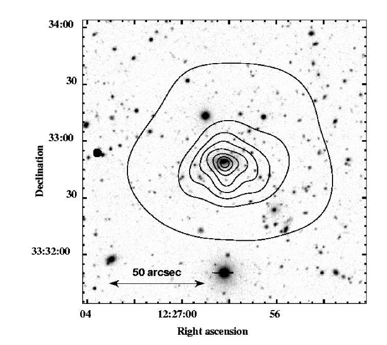
Figure 3: Contours of X-ray emission detected by Chandra ($0.5-5\mbox{$\mathrm{~{}keV}$}$) overlaid on the same Subaru I-Band image as Fig 2. The contours are taken from an exposure-corrected image that was adaptively smoothed so that all features were significant at the $99\%$ level. The contours are logarithmically spaced above the lowest contour at $0.03\mathrm{~{}counts~{}pixel^{-1}}$.

3.1 Two-dimensional modelling of the X-ray emission

A two-dimensional (2D) model of the X-ray emission was fit to the XMM-Newton data, taking the different background components and instrumental effects into account. The approach followed was to bin the data into an image with $4.4\mathrm{{}^{\prime}}\hskip-1.00006pt\mathrm{{}^{\prime}}$ pixels, but apply no vignetting correction, or any further manipulation of the data. This pixel size was chosen so as to be an integer multiple of the $1.1\mathrm{{}^{\prime}}\hskip-1.00006pt\mathrm{{}^{\prime}}$ pixels of the point spread function (PSF) images produced by the SAS tool calview, allowing them to be re-binned to the same scale, and to be large enough to reduce computing time in the fitting procedure, without losing resolution. An image of a dataset obtained with the filter in the closed position (and thus blocking all X-rays) was filtered in the same way as the source data, and normalised to it, using the ratio of outside field-of-view counts in the two sets, creating a ‘particle image’. This was smoothed with a Gaussian of $\sigma=20\mathrm{{}^{\prime}}\hskip-1.00006pt\mathrm{{}^{\prime}}$ to prevent the fitting being biased by noise, while maintaining any larger scale spatial variation of this background component. The particle image was then divided by an exposure map, giving an anti-vignetted image of the particle component of the background. The exposure map was also used to make a binary filter mask to exclude the CCD gaps and bad pixels from the fit.

In a background region of the data (on the same CCD where possible), a model comprised of the anti-vignetted particle image in that region, plus a flat component to represent the X-ray background, were multiplied by the exposure map, convolved with the PSF, and fit to the data, with both background component normalisations free to vary. This meant that in effect, the background was fit with a flat particle background, and a vignetted X-ray plus soft-proton background. We note that the best-fitting normalisation of the particle background varied by less than $5\%$ from its initial value. This indicates that the normalisation to the outside field-of-view events was accurate, and therefore the vignetted-background level found here should also be accurate. These background normalisations were then fixed, and the source was modelled with the anti-vignetted particle image in the source region, plus a flat X-ray background, plus a 2D $\beta$-profile, all multiplied by the exposure map and convolved with the PSF.

This procedure was followed for the PN and MOS cameras, and then the fits were performed simultaneously, with each of the three models using their appropriate exposure map, fitted background levels, and PSF (images of the PSF of each telescope were generated at $1.5\mbox{$\mathrm{~{}keV}$}$, corresponding to the peak effective area, and at an appropriate off-axis angle). The amplitudes of the models were independent, but they were constrained to fit to the same slope, core radius, central position, ellipticity, and rotation angle. The best-fitting model had a core radius $r_{c}=14.5^{+1.2}_{-0.8}{\mathrm{{}^{\prime}}\hskip-1.00006pt\mathrm{{}^{\prime}}}$, a slope $\beta=0.66^{+0.02}_{-0.02}$, and an ellipticity of $0.14$ (while all parameters were free to vary in the error computation, errors were only computed on $r_{c}$ and $\beta$ because of the computational load involved). The fitting was repeated with the PN and combined MOS data separately, and the best-fitting parameters were found to be consistent throughout.

3.2 One-dimensional surface-brightness profile

In order to measure the extent of the emission, and to investigate the goodness-of-fit of the 2D model to the data, a one-dimensional (1D) surface-brightness profile of the emission in an exposure corrected, combined image from the three XMM-Newton EPIC cameras was produced. Before the exposure correction, the exposure maps were normalised to their value at the cluster centroid, thereby maintaining, as much as possible, the Poissonian statistics in an exposure-corrected image.

The profile was centred on the X-ray centroid ($\alpha[2000.0]=12^{\rm h}26^{\rm m}57.94^{\rm s}$, $\delta[2000.0]=+33^{\circ}32\mathrm{{}^{\prime}}46.2\mathrm{{}^{\prime}}\hskip-1.00006pt\mathrm{{}^{\prime}}$), and the circular radial bins were adaptively sized so that each contained a detection with a signal-to-noise ratio of at least 3 (the background level being estimated from a large concentric annulus - we note that this is likely to be an overestimate of the background at the cluster centre, due to the anti-vignetted particle background). The emission was detected out to $100\mathrm{{}^{\prime}}\hskip-1.00006pt\mathrm{{}^{\prime}}$ ($776\mbox{$\mathrm{~{}kpc}$}$) at the $3\sigma$ level.

The 2D analysis is superior to the 1D analysis, not least because we do not account for the PSF in the 1D analysis. We can however test the goodness of fit of the 2D model in the following way. A 1D profile of the best-fitting 2D model convolved with the PSF was made, and compared to the observed 1D profile. A 1D $\beta$-model (Cavaliere & Fusco-Femiano, 1976) plus a flat background was fit to both the profile of the data and the 2D model and the best-fitting parameters were in good agreement. In the fit to the data, the reduced $\chi^{2}$ was $1.09$ for $53$ degrees of freedom. The best-fitting 1D models to the data and 2D model are overlaid on a profile of the data in fig 4. These comparisons indicate that the 2D model provides a good description of the data.

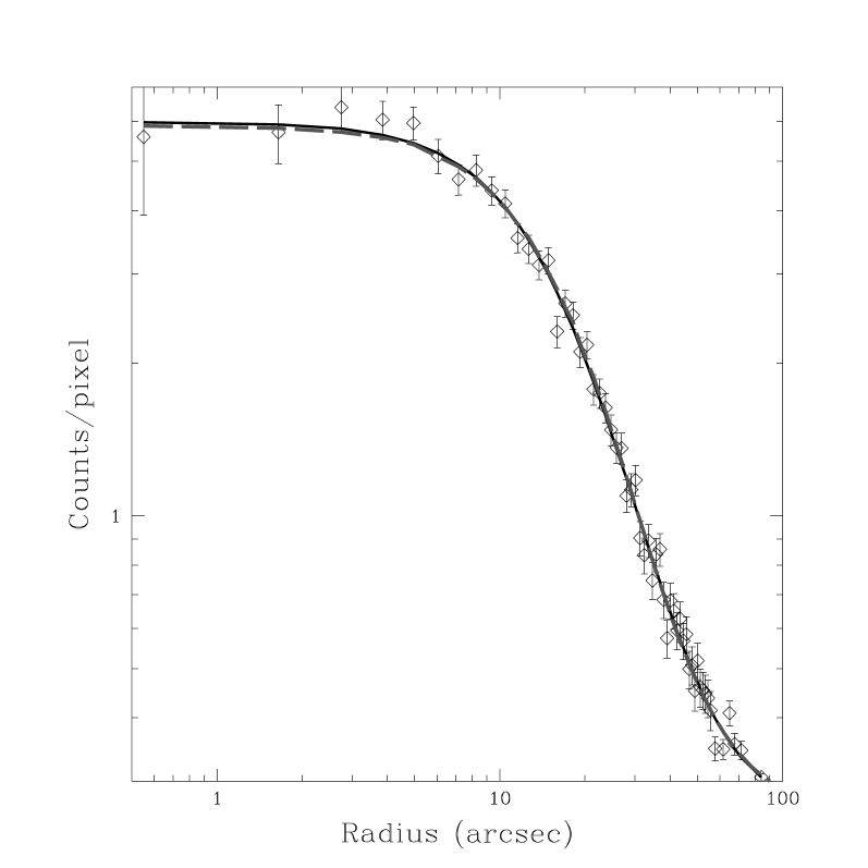
Figure 4: Adaptively binned XMM-Newton surface-brightness profile of ClJ1226.9$+$3332, with each bin containing a signal-to-noise ratio of at least three. The lines show the best-fitting 1D model to the data (solid line) and two-dimensional model (dashed line).

3.3 Chandra analysis and the central region

The archived Chandra observation of ClJ1226.9$+$3332 was also subjected to a similar 1D and 2D analysis, and the best-fitting model parameters were consistent with those derived from the XMM-Newton data, but of lower statistical precision.

Many relaxed clusters show excess emission above a $\beta$-model due to cool, dense gas in central regions, previously referred to as a cooling flow (Fabian, 1994). The residuals of the XMM-Newton and Chandra data after subtraction of the best-fitting 2D models were examined, and while both showed a weak central excess, these features were not statistically significant. Excluding the central regions ($r<5\mathrm{{}^{\prime}}\hskip-1.00006pt\mathrm{{}^{\prime}}$ for Chandra, $r<20\mathrm{{}^{\prime}}\hskip-1.00006pt\mathrm{{}^{\prime}}$ for XMM-Newton, consistent with the PSF) in the profile fits also gave no significant change to the best-fitting model parameters.

3.4 Hardness-ratio Mapping

The temperature structure of the cluster was probed with hardness-ratio mapping. The hardness ratio, HR, was defined as

$$HR = \frac{H-AH_{bg}}{S-AS_{bg}},$$ (1)

where $H$ and $S$ are the counts in the source region in the hard and soft band respectively, and the $bg$ subscript indicates the counts found in a background region. $A$ is the ratio of the area of the source region to the background region. Assuming that the errors on each pixel are Poissonian and uncorrelated, the error on the hardness ratio is then given by

$$\sigma(HR)^{2} = \frac{H+A^{2}H_{bg}}{(S-AS_{bg})^{2}}+\frac{(H-AH_{bg})^{2}(S+A^{2}S_{bg})}{(S-AS_{bg})^{4}}.$$ (2)

A soft band of $0.3-1.1\mbox{$\mathrm{~{}keV}$}$, and a hard band of $1.1-8\mbox{$\mathrm{~{}keV}$}$ were chosen when computing the ratios because these band had similar numbers of net counts. Images of the cluster emission produced in these hard and soft bands were binned up adaptively, in order to maximise the signal to noise in each bin while maintaining good resolution. The minimum number of background-subtracted counts ($0.3-8\mbox{$\mathrm{~{}keV}$}$) was set to $150$ per bin, although a few bins were allowed to fall below this threshold to improve the resolution. The resultant images were then divided to give a hardness-ratio map. A series of absorbed MeKaL spectra were simulated at different temperatures (assuming a constant Galactic absorption of $1.38\times 10^{20}\mbox{$\mathrm{~{}cm^{-2}}$}$ (Dickey & Lockman, 1990), and fixed metallicity of $0.3\mathrm{Z_{\odot}}$), convolved with the appropriate instrument responses, and the number of counts in the hard and soft bands were found. This enabled the conversion between HR values and approximate temperatures.

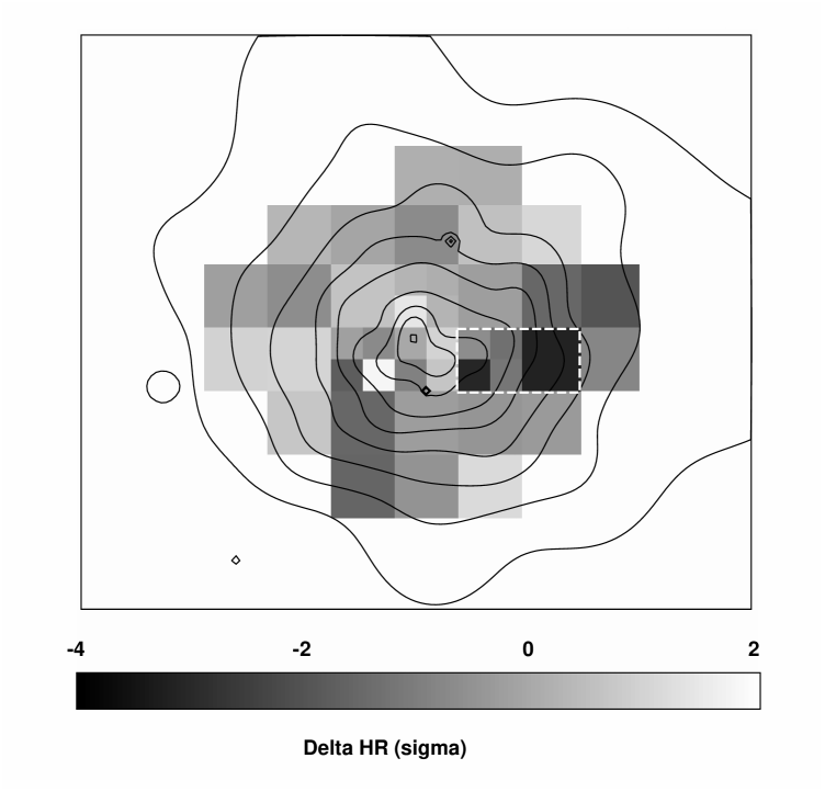
Figure 5: Adaptively binned HR significance map of the XMM-Newton data. The overlaid contours are the same as in Fig. 2. The dashed box contains regions of significantly lower temperature than the mean, assuming no variation in absorbing column.

Fig. 5 is an image of the differences between the HR in each bin from the HR corresponding to the global spectrally-measured temperature ($11.5\mbox{$\mathrm{~{}keV}$}$; see §5) divided by the errors on both the local HR and the HR of the global temperature added in quadrature. Pixels where the broadband net counts were $<50$ are excluded, and the remaining pixels have an average of $140$ counts. This significance map shows that, within the limits of the data, the emission is generally isothermal; $66\%$ of the pixels are within $1\sigma$ of the HR corresponding to the global temperature, and $95\%$ are $<2\sigma$ from this HR.

A region of significantly cooler emission to the west of the cluster centre is marked with a white, dashed box in Fig. 5. The two darkest pixels here are just over $3\sigma$ softer than the global temperature HR (note that we would expect only $0.12$ pixels to be $>3\sigma$ from the mean if they were randomly distributed). Spectra were extracted within this region, and fit with an absorbed MeKaL model. The best-fitting temperature was $6.5^{+1.2}_{-1.0}\mbox{$\mathrm{~{}keV}$}$ with the abundance frozen at $0.3\mathrm{Z_{\odot}}$, or $5.9^{+1.1}_{-0.9}\mbox{$\mathrm{~{}keV}$}$ with a poorly constrained abundance of $0.8\mathrm{Z_{\odot}}$. The reduced $\chi^{2}$ in both cases was $1.3$ for $29$ (or $28$) degrees of freedom, suggesting that, though the statistical errors are large, a simple MeKaL model is not a good description of the emission from this region (it is excluded at the $88\%$ level). The Chandra data indicate that point source contamination is unlikely; a more likely cause is multi-temperature gas in this region. A plausible explanation is that we are observing the in-fall of some cooler ($<6\mbox{$\mathrm{~{}keV}$}$) body, whose emission is mixed with that from the hotter gas along the line of sight.

4 Spectral analysis methods

When performing spectral analysis, one must be particularly careful to treat the background components correctly, as failing to do so can strongly influence the results. We have performed a thorough investigation of different methods of treating the background spectra, which are in general extracted in one of two ways. One may extract a local background spectrum from a large region of the same CCD as the source emission. This method has the disadvantage that instrumental features in the background spectrum and the response of the detectors vary across the CCD, and the background spectrum will be more severely vignetted than the source spectrum, tending to come from further off-axis.

Alternatively, one may use a background spectrum extracted from a blank-sky dataset, which is a combination of several observations with all bright sources removed. This method has the advantage that the spectrum can be extracted from the same detector region as the source spectrum, and that the effective exposure time of the blank-sky dataset can be many times longer than that of the observation, reducing the Poissonian errors on the background spectrum. The disadvantages of this method are that the blank-sky observations are taken at different times and pointings to the source data, and the background varies both directionally and temporally. In particular the soft X-ray background varies directionally due to absorption in the galaxy, and emission from the local bubble, while the shape and amplitude of the non-X-ray background spectrum varies temporally due to soft-proton flaring events, and variations in the particle flux.

In principle, one can compensate for the vignetting of the telescope by weighting each event (using SAS 5.3’s evigweight). The weight is derived from the ratio of the effective area at the position and energy of each event, to the effective area at that energy on-axis. This method is described in detail by, for example, Arnaud et al. (2002). The disadvantage of applying this weighting is that non-vignetted particle induced events are also weighted, artificially boosting their contribution. This effect can be avoided when using a blank-sky background because the source and background spectra are extracted from the same detector region. Providing that the particle contribution is the same in the source and blank-sky datasets, then the particle weighting effect will be the same, and its effect will cancel when the spectra are subtracted. The spectra produced from these weighted datasets should resemble the spectra one would detect with a flat detector, so the on-axis Ancillary Response File is used when performing the spectral fitting.

Thus four spectral background methods were investigated; local and blank-sky backgrounds, with and without weighting. These methods were applied to the low background and high background periods (see §2), and both periods combined. In each case, the source spectrum was extracted from a circle of radius $100\mathrm{{}^{\prime}}\hskip-1.00006pt\mathrm{{}^{\prime}}$ centred on the cluster centroid. We note that this region crosses a PN CCD gap, but the responses of the PN CCDs are identical, and do not vary strongly across the chip, so this should not present a significant source of uncertainty. The spectra were all fit with an absorbed MeKaL model, in the range $0.3-8\mbox{$\mathrm{~{}keV}$}$, with abundances fixed at $0.3\mathrm{Z_{\odot}}$ and the absorbing column density fixed at the Galactic value of $1.38\times 10^{20}\mbox{$\mathrm{~{}cm^{-2}}$}$ (Dickey & Lockman, 1990).

4.1 The Low Background Period

All of the background methods described below gave temperatures consistent with $11.5\pm 2\mbox{$\mathrm{~{}keV}$}$. We take this as a reliable measurement of the temperature, free of systematic errors, but now check the results when, in addition, the high background period is included.

4.2 Local background, no weighting

This method is the most straightforward, and given the high background level in this dataset, is likely to be the most reliable. A background spectrum was extracted from a large region of the same CCD, at $\approx 250\mathrm{{}^{\prime}}\hskip-1.00006pt\mathrm{{}^{\prime}}$ from the cluster centre. This was far enough to avoid contaminating emission, but as close as possible to reduce the difference in effective area between the source and background regions. The best-fitting temperature was $T=11.56\pm 1.26\mbox{$\mathrm{~{}keV}$}$ with a reduced $\chi^{2}/dof=0.93/298$. We also investigated the dependence of the result on the background region chosen, by using two other background regions, and the best-fitting temperatures were all consistent within their $1\sigma$ errors.

4.3 Local background, with weighting

This method is similar to the preceding one, except the spectrum is produced from weighted events, as described above. This method should reduce the discrepancy between the effective area at the source region and the background region. However the contribution of particle induced events will be incorrectly boosted, and will be boosted more strongly in the background region which is further off-axis.

We extracted weighted source and background spectra from the same regions used above. The best-fitting temperature was $T=4.44\pm 0.49\mbox{$\mathrm{~{}keV}$}$ (reduced $\chi^{2}/dof=1.15/340$), significantly lower than that found with the non-weighted spectrum above. This suggests that the anti-vignetting of the particle events, combined with their high level, has a strong effect in these data.

4.4 blank-sky background, no weighting

This method uses a spectral background taken from the same detector region as the source spectrum, in a blank-sky dataset. The high background level in the source dataset means that its spectrum may be quite different from that of the blank-sky dataset. We attempt to account for this with the following method, based closely on that used by Arnaud et al. (2002). Briefly, the blank-sky background was scaled to the data using the ratio of the count rates in the whole field of view in the $12-14\mbox{$\mathrm{~{}keV}$}$ band. A spectrum obtained from a background region of the data was subtracted from a corresponding blank-sky spectrum to produce a ‘residual spectrum’. This was subtracted from the blank-sky spectra to account for systematic residuals between the data and the blank-sky spectra. Generally, the residual spectrum is taken from further off-axis than the source, so will be more strongly vignetted. This means that any soft X-ray excess (or decrement) in the source data will be underestimated (or overestimated) to some extent.

Spectra produced with this method were fit as before, giving a temperature of $T=11.48\pm 1.45\mbox{$\mathrm{~{}keV}$}$ (reduced $\chi^{2}/dof=0.96/298$), in excellent agreement with the temperature found with the non-weighted local background method above ($T=11.56\pm 1.26\mbox{$\mathrm{~{}keV}$}$).

4.5 blank-sky background, with weighting

The problem of the vignetting of the residual spectrum in the preceding method can be solved, in theory, by applying the weightings defined above to the source and blank-sky datasets, before following the method described in the preceding section. Again, the particle induced events will be artificially boosted by the weighting, but in this case, as the source and background spectra are extracted from the same regions, the boosting factor should be the same, and it will cancel, providing that the particle event level in the source and blank-sky sets are similar. Weighted spectra were produced, following the method above, and the best-fitting model had a temperature of $T=7.79\pm 1.12\mbox{$\mathrm{~{}keV}$}$ (reduced $\chi^{2}/dof=1.15/340$). This is not consistent with the temperature found by the two non-weighted methods, suggesting again that the boosting of the particle events is a significant effect.

4.6 Spectral analysis - summary and conclusions

When applied to the low background data, all spectral analysis methods gave a temperature consistent with $11.5\mbox{$\mathrm{~{}keV}$}$, with $1\sigma$ errors of $\approx\pm 2\mbox{$\mathrm{~{}keV}$}$. We believe that this consistency between the methods is due to the lower particle background in this period. In both the high background period, and combined periods, the results were consistent with the low background period when no weightings were used. We believe that the inconsistencies that emerged when weighting methods were used was due to the boosting of the higher particle levels in these data. In a further test, the absorbing column was allowed to vary, along with the temperature, in our analysis of the combined period data. The Galactic value at the position of ClJ1226.9$+$3332 is $1.38\times 10^{20}\mbox{$\mathrm{~{}cm^{-2}}$}$ (Dickey & Lockman, 1990); the best-fitting value with a local background spectrum was $1.6\pm 0.7\times 10^{20}\mbox{$\mathrm{~{}cm^{-2}}$}$ ($T=11.33\pm 1.55$), while with a blank-sky background spectrum, the best fit was $5.0\pm 1.0\times 10^{20}\mbox{$\mathrm{~{}cm^{-2}}$}$ ($T=9.05\pm 1.18$). This again shows the reliability of the local background method. All further analysis was performed on the combined period data, with a local background as this approach gives the best compromise between limiting systematic and statistical sources of uncertainty for these data. The non-weighted blank-sky method was used as a consistency check.

5 Spectral results

The results of the fits to various combinations of the three XMM-Newton cameras are given in table 1. All quoted results were found using a local background with no weighting, though in each case, consistent results were found using a blank-sky background. All spectral fits for all combinations of cameras gave consistent results. The spectra were fit in the $0.3-8\mbox{$\mathrm{~{}keV}$}$ band, though we note that consistent results were also found when fitting in the $1-7\mbox{$\mathrm{~{}keV}$}$ band.

Camera	$T(keV)$	Reduced $\chi^{2}/dof$
PN	$11.56\pm 1.26$	$0.93/298$
MOS1	$12.42\pm 2.80$	$0.98/98$
MOS2	$11.93\pm 1.76$	$0.98/103$
MOS1+MOS2	$12.28\pm 1.89$	$0.99/203$
PN+MOS1+MOS2	$11.55\pm 0.86$	$1.00/503$

Table 1: Summary of the results of spectral fits to different combinations of the XMM-Newton cameras with a local background and no weighting. The temperatures quoted were derived from spectral fits with abundances frozen at $0.3$ solar, and the absorbing column frozen at the Galactic value.

The simultaneous fit to the data from all three cameras was then investigated in more detail, with the abundance as a free parameter. The best-fitting model was $T=11.5^{+1.1}_{-0.9}\mbox{$\mathrm{~{}keV}$}$ and $Z=0.33^{+0.14}_{-0.10}\mathrm{Z_{\odot}}$ (reduced $\chi^{2}=1.07$ for $502$ degrees of freedom); this abundance is well constrained for a high-redshift cluster, and is in good agreement with that found in local clusters (the blank-sky method gave an abundance of $Z=0.37^{+0.17}_{-0.17}\mathrm{Z_{\odot}}$). Fig. 6 shows the best-fitting PN and MOS spectra, produced using a local background. The spectra were grouped so that each bin contained a minimum of 50 counts (PN) or 20 counts (MOS).

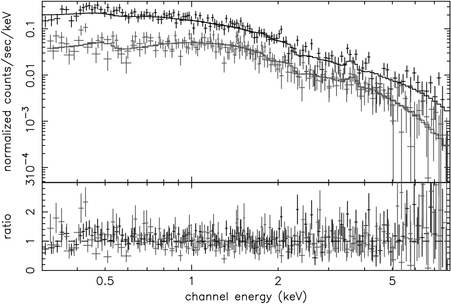
Figure 6: PN (upper) and MOS (lower) spectra with the best-fitting model. The ratio of data to model values is shown in the lower panel. A local background spectrum was used.

The flux of ClJ1226.9$+$3332 measured by ROSAT in the $0.5-2\mbox{$\mathrm{~{}keV}$}$ passband was $3.4\pm 0.3\times 10^{-13}\mathrm{\mbox{$\mathrm{~{}erg}$}\mathrm{\mbox{$\mathrm{~{}s}$}^{-1}}\mbox{$\mathrm{~{}cm^{-2}}$}}$. For comparison, the XMM-Newton flux in this band was $3.7^{+0.1}_{-0.1}\times 10^{-13}\mathrm{\mbox{$\mathrm{~{}erg}$}\mathrm{\mbox{$\mathrm{~{}s}$}^{-1}}\mbox{$\mathrm{~{}cm^{-2}}$}}$ (after extrapolation to $r_{\mathrm{200}}$).

5.1 Temperature Profile

A temperature profile was created by fitting spectra extracted from annular bins centred on the X-ray centroid. In order to minimise the effect of the PSF, while maintaining a degree of spatial resolution, the annuli were chosen so that their width (or diameter in the case of the innermost bin) were $\geq 15\mathrm{{}^{\prime}}\hskip-1.00006pt\mathrm{{}^{\prime}}$, which corresponds to the $70\%$ encircled energy radius of the PSF. Spectra were fit as before in each of these annular bins, freezing the abundance at $0.3\mathrm{Z_{\odot}}$ and the column density at the Galactic value, using a local background, and fitting in the $0.3-8\mbox{$\mathrm{~{}keV}$}$ band. The temperature profile is shown in Fig. 7. The profile is consistent with isothermality, albeit with large errors, and shows no sign of any central cool gas.

The effect of the projection of the emission from the gas in the outer annuli was then modelled with an ‘onion skin’ method. The temperature structure was modelled as a series of spherical shells (each of which was isothermal), and the spectra were fit from the outermost shell in. The spectrum of a shell was modelled with a single temperature MeKaL component, plus a MeKaL component for each external shell, whose temperature was fixed at the value measured in that shell, and whose normalisation was multiplied by a factor. These factors accounted for the volume of each external shell along the line of sight to the shell being fit, and the variation in density across each external shell using the measured gas density profile. This deprojection procedure had no significant effect on the form of the temperature profile, and did not reveal any central cool gas, although the size of the errors was increased, as one would expect, as there were less photons available to constrain the temperature of the free component in the interior bins.

Figure 7: Temperature profile of ClJ1226.9$+$3332, based on spectra fit with abundance frozen at $0.3\mathrm{Z_{\odot}}$, and a locally extracted background. Projected and deprojected temperatures are plotted, with the deprojected points offset by $2\mathrm{{}^{\prime}}\hskip-1.00006pt\mathrm{{}^{\prime}}$ for clarity. The solid line is the best-fitting global temperature, with $1\sigma$ errors represented by the dashed lines.

5.2 Entropy Profile

The measurement of the gas entropy in groups and clusters of galaxies has provided evidence for some form of non-gravitational heating (e.g. Ponman et al., 1999; Lloyd-Davies et al., 2000; Ponman et al., 2003). In particular, if the entropy profiles of all systems are scaled by temperature, then cooler systems have a higher scaled entropy than hotter systems. This contrasts with the predictions of self-similar models, which include only gravitational heating, where all scaled-entropy profiles are identical. This indicates that non-gravitational heating has an impact in cooler systems where it provides a significant fraction of the gas energy, while its effect is not detectable in hotter systems. One would expect then, that an extremely hot system such as ClJ1226.9$+$3332 would have a similar entropy profile to other hot systems, and our temperature profile of this system allowed a rare opportunity to measure an entropy profile at high redshift.

For consistency with other work (Ponman et al., 1999; Lloyd-Davies et al., 2000; Ponman et al., 2003), we defined a pseudo-entropy,

$$S = T/n_{e}^{2/3}\mathrm{\mbox{$\mathrm{~{}keV}$}\mathrm{\mbox{$\mathrm{~{}cm}$}^{2}}}.$$ (3)

It was then straightforward to produce the entropy profile shown in Fig. 8, using the gas density determined from the surface-brightness profile. The entropy was calculated assuming gas isothermality at $11.5\mbox{$\mathrm{~{}keV}$}$, and the data points show the entropies derived from the measured temperatures in the projected temperature profile.

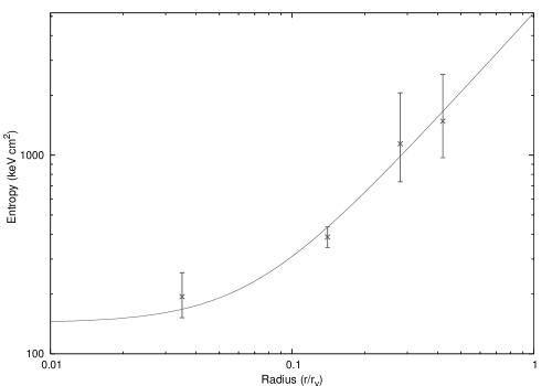
Figure 8: Gas entropy of ClJ1226.9$+$3332 versus radius as a fraction of $r_{\mathrm{200}}$. The gas was assumed to be isothermal at $11.5\mbox{$\mathrm{~{}keV}$}$, and the data points give the entropies computed from the measured deprojected temperatures shown in Fig. 7.

It is interesting to note that the entropy observed at $0.1r_{\mathrm{200}}$ ($\approx 300\pm 40\mathrm{\mbox{$\mathrm{~{}keV}$}\mathrm{\mbox{$\mathrm{~{}cm}$}^{2}}}$) is significantly lower than that found in local systems of similar temperature at this radius. For example Ponman et al. (2003) find an entropy of $\approx 550\pm 50\mathrm{\mbox{$\mathrm{~{}keV}$}\mathrm{\mbox{$\mathrm{~{}cm}$}^{2}}}$ in local systems above $10\mbox{$\mathrm{~{}keV}$}$. This lower entropy could be explained by an underestimate of the temperature of ClJ1226.9$+$3332, however the temperature required to bring the entropy in line with the local systems is $\approx 17\mbox{$\mathrm{~{}keV}$}$, which seems unlikely. On the other hand, the central electron density could be overestimated here. The measured value of $n_{e}$ was $0.0228\pm 0.001\mbox{$\mathrm{~{}cm^{-2}}$}$, and a reduction of $\approx 50\%$ is required to bring the entropy at $0.1r_{\mathrm{200}}$ in line with local values. As discussed in Section §6, the value of $r_{\mathrm{200}}$ used here is subject to systematic uncertainties due to the assumptions made in extrapolating the mass profile. However, these tend to lead to an overestimate of $r_{\mathrm{200}}$, giving an overestimate of the entropy at $0.1r_{\mathrm{200}}$ so this is unlikely to be the cause of the difference between the entropy in local systems and that observed here.

An alternative explanation is that we are observing entropy evolution, driven by the increasing density of the universe with redshift. Assuming simple self-similar scaling, the mean density within a given overdensity radius (relative to the critical density) is proportional to $H(z)^{2}$. The electron density then scales with redshift as

$$n_{e}(z) \propto H_{0}^{2}E(z)^{2},$$ (4)

where

$$E(z) = (1+z)\left(1+z\Omega_{M}+\frac{\Omega_{\Lambda}}{(1+z)^{2}}-\Omega_{\Lambda}\right)^{1/2}.$$ (5)

Assuming that the redshift of observation is similar to the redshift of formation (or at least, the redshift at which the systems last virialised after a major merger), entropy, when scaled by system temperature, should therefore evolve as $E(z)^{-4/3}$. If the measured entropy in ClJ1226.9$+$3332 at 0.1$r_{v}$ is scaled by this factor (to give 588$\pm$78 keV cm²), it is consistent with, the local (Ponman et al., 2003) value. We note that if the dependence of the density contrast $\Delta_{c}(z)$ on cosmology and redshift (as described by Bryan & Norman (1998)) is included in the redshift-scaling of the ClJ1226.9$+$3332 entropy, its value is slightly higher than, but still consistent with, the local (Ponman et al., 2003) value. This suggests that simple, self-similar arguments may explain ICM entropy evolution. Future papers will examine the evolution of entropy and other scaling relations using a sample of high-redshift clusters.

5.3 Chandra spectral analysis

A spectrum was also extracted from the archived Chandra observation of ClJ1226.9$+$3332, within a $60\mathrm{{}^{\prime}}\hskip-1.00006pt\mathrm{{}^{\prime}}$ radius circle, and with a background extracted from a large concentric annular region of the S3 chip (excluding point sources). The quantum efficiency (QE) degradation suffered by Chandra since launch can cause significant overestimates of cluster temperatures if not modelled correctly (e.g. Maughan et al., 2003). To account for this, the Chandra spectrum was fit with an absorbed MeKaL model, including an extra ACISABS absorption component. The observation of ClJ1226.9$+$3332 was taken $376$ days after launch. There are also uncertainties in the cross-calibration of the quantum efficiency of the front-illuminated (FI) and back-illuminated (BI) CCDs. It was initially thought that the QE curves were overestimated at low energies by $\approx 7\%$ for the FI chips. A more recent reanalysis of pre-flight data has shown that the QE curves of the BI chips are underestimated by $\approx 9\%$. However, due to an additional (as yet unreleased) correction that is required to the telescope effective area, the current best advice for measuring an accurate temperature using the back-illuminated S3 chip is not to apply any additional QE correction. Accordingly, none was applied, but we note that systematic uncertainties at the $\approx 10\%$ level may exist.

The fits were performed in the $0.6-8\mbox{$\mathrm{~{}keV}$}$ band, with the column density frozen at the Galactic value, and the abundance at $0.3\mathrm{Z_{\odot}}$. The best-fitting model temperature was $12.6^{+3.0}_{-2.2}\mbox{$\mathrm{~{}keV}$}$, in good agreement with that measured by XMM-Newton. The best-fitting Chandra temperature was also found to be consistent when the spectrum was fit in the $1-8\mbox{$\mathrm{~{}keV}$}$ band, where the effects of the quantum efficiency degradation are less severe.

The unabsorbed flux measured by Chandra ($0.5-2\mbox{$\mathrm{~{}keV}$}$) was $3.6\pm 0.1\times 10^{-13}\mathrm{\mbox{$\mathrm{~{}erg}$}\mathrm{\mbox{$\mathrm{~{}s}$}^{-1}}\mbox{$\mathrm{~{}cm^{-2}}$}}$ (after extrapolation to $r_{\mathrm{200}}$), which is consistent with that measured by XMM-Newton and ROSAT . This shows again that point source contamination was not a problem in the XMM-Newton data.

6 Determination of Global Properties

We have derived the luminosity, gas mass, total mass, and gas mass fraction within two different radii. The most reliable results are those obtained within the extent of the data ($r=100\mathrm{{}^{\prime}}\hskip-1.00006pt\mathrm{{}^{\prime}}$, corresponding to an overdensity $\Delta\approx 1000$). The easiest results to compare with theoretical models of cluster growth are those extrapolated by a factor of $2.2$ in radius to $r_{\mathrm{200}}$, but systematic uncertainties may be associated with the extrapolation.

The method used was similar (but not identical) to that described in Maughan et al. (2003). Briefly, if the gas density profile is described by a $\beta$-model, then under the assumptions of isothermality, hydrostatic equilibrium, and spherical symmetry, the total density profile of the cluster is given by

$$\bar{\rho}(<r) = \frac{M(<r)}{4/3\pi r^{3}}$$ (7)

$$= 2.70\times 10^{13}\beta\frac{T}{\mbox{$\mathrm{~{}keV}$}}\left(\frac{r}{\mbox{$\mathrm{~{}Mpc}$}}\right)^{-2}\times$$

$$\frac{(r/r_{c})^{2}}{1+(r/r_{c})^{2}}M_{\odot}\mbox{$\mathrm{~{}Mpc}$}^{-3}.$$

Here, we have adopted a value of $0.59m_{p}$ for the mean molecular weight of the gas, where $m_{\rm p}$ is the proton mass. This density profile was used to estimate $r_{\mathrm{200}}$, and the measured flux was extrapolated out to this radius, and converted to a luminosity. The central gas density was computed from the measured MeKaL normalisation, and the measured gas density profile was integrated to give the gas mass. The total gravitating mass within $r_{\mathrm{200}}$ was derived from Eqn. 7.

The errors quoted on all non-observed quantities were derived from $10,000$ randomisations of the measured quantities under the Gaussians described by their measured $1\sigma$ errors. The properties of ClJ1226.9$+$3332 are summarised in Table 2. Our assumption of isothermality is supported by the measured temperature profile, and hardness-ratio mapping, while the relaxed appearance of the X-ray emission, and the good fit of an isothermal $\beta-$model to the data indicate that the gas is close to hydrostatic equilibrium.

The extrapolation of the cluster properties out to large radii introduces systematic uncertainties which are not taken into account in the above method. In a sample of 66 systems with measured temperature profiles Sanderson et al. (2003) found that the incorrect assumption of isothermality leads to an average overestimate of $M_{200}$ by $\approx 30\%$ and $r_{\mathrm{200}}$ by $\approx 20\%$. The overestimation of $r_{\mathrm{200}}$ leads in turn to an overestimation of $M_{gas}$ by $\approx 25\%$ at that radius (the $r_{\mathrm{200}}$ and $M_{gas}$ uncertainties were provided by Sanderson (private communication)). These are taken as reasonable indications of the systematic uncertainties on those properties, and are added in quadrature to the statistical errors derived above in the quoted values of these properties.

We find a virial radius of $r_{\mathrm{200}}=1.66\pm 0.34\mbox{$\mathrm{~{}Mpc}$}$ for cluster ClJ1226.9$+$3332. This means that the properties of the system are directly measured out to $\approx 0.45r_{\mathrm{200}}$. Assuming an extrapolation of the surface-brightness profile is valid, it is interesting to note that while this radius encloses $90\%$ of the X-ray emission, it encloses only $\approx 45\%$ of the gas mass and total mass of the system.

$\Delta$	Redshift	$T(keV)$	$L_{bol}(erg\mbox{$\mathrm{~{}s}$}^{-1})$	$\sigma(\mathrm{\mbox{$\mathrm{~{}km}$}\mathrm{\mbox{$\mathrm{~{}s}$}^{-1}}})$	$r_{c}({\mbox{$\mathrm{~{}kpc}$}})$	$\beta$	$r_{\Delta}(Mpc)$	$M_{gas}(M_{\odot})$	$M_{tot}(M_{\odot})$	$f_{gas}$
1000	$0.892$	$11.5^{+1.1}_{-0.9}$	$4.8\pm 0.1\times 10^{45}$	$997^{+285}_{-205}$	$113^{+9}_{-6}$	$0.66^{+0.02}_{-0.02}$	$0.73\pm 0.04$	$6.5\pm 0.4\times 10^{13}$	$6.1^{+0.9}_{-0.8}\times 10^{14}$	$0.11\pm 0.02$
200			$5.3\pm 0.2\times 10^{45}$				$1.66\pm 0.34$	$1.7\pm 0.4\times 10^{14}$	$1.4\pm 0.5\times 10^{15}$	$0.12\pm 0.05$

Table 2: Summary of the measured and inferred properties of cluster ClJ1226.9$+$3332 based on XMM-Newton observations, assuming a cosmology of $\Omega_{M}=0.3$ $(\Omega_{\Lambda}=0.7)$ and $H_{0}=70$$\mathrm{\mbox{$\mathrm{~{}km}$}\mathrm{\mbox{$\mathrm{~{}s}$}^{-1}}\mathrm{\mbox{$\mathrm{~{}Mpc}$}^{-1}}\,}$. The first line gives the properties within the detection radius, corresponding to an overdensity of $\Delta=1000$. The second line gives the properties when extrapolated to an overdensity radius of $\Delta=200$.

7 Velocity Dispersion

ClJ1226.9+3332 was observed by us on April 18, 2002 with the LRIS spectrograph (Oke et al., 1995) on the Keck-I 10m telescope. We used the 600 l/mm grism blazed at $1\micron$, and a multi-object spectroscopy mask with 1.25” wide slits. Further details of the observational setup and the data reduction procedure will be provided in a future paper (Ebeling et al., 2003). From 12 accurately measured cluster redshifts (individual radial velocity error less than 30 km s^-1) and using a biweight estimator for the systemic cluster redshift $z$ and the comoving cluster velocity dispersion $\sigma$ we find $z=0.8920$ and $\sigma=997^{+285}_{-205}\mathrm{\mbox{$\mathrm{~{}km}$}\mathrm{\mbox{$\mathrm{~{}s}$}^{-1}}}$ using the ROSTAT statistics package (Beers et al., 1990).

The observed velocity dispersion is consistent with the measured X-ray temperature, given the scatter in the local $T-\sigma$ relation of Xue & Wu (2000) The velocity histogram, although poorly constrained with only 12 velocities, shows no signs of significant substructure.

8 Discussion

ClJ1226.9$+$3332 is the highest temperature galaxy cluster known at $z>0.6$, and, uniquely at these redshifts, is an extremely massive system (similar in mass to the Coma cluster) which appears to be relaxed. Images of both the XMM-Newton observation analysed here, and the archived Chandra observation show almost circular isophotes, and no obvious large-scale substructure. Within the limits of the current data, the cluster is generally isothermal (except for one small cooler region). The relaxed nature is further supported by the good agreement of the $\beta$-model with the surface brightness distribution. This relaxed appearance is important in justifying the assumptions used to derive the total mass.

The existence of even one high-redshift cluster of this mass can be used to constrain cosmological models. We initially test for consistency with the $\Lambda$CDM cosmology of Spergel et al. (2003) from Wilkinson Microwave Anisotropy Probe (WMAP) data, using their results based on a model with a constant spectral index of primordial fluctuations. In this cosmology, at a redshift of $0.89$ we expect to see a density of systems more massive than CLJ$1226.9+3332$ of $4.86\times 10^{-3}$ deg^-2 per unit $z$. We have adopted the Jenkins et al. (2001) halo mass function in this calculation, and converted between our mass definition ($M_{200}$ relative to the critical density) and that of Jenkins et al. (2001) ($M_{180}$ relative to the background density) via: $M_{180}/M_{200}=1.14$, assuming an NFW (Navarro et al., 1996) profile with concentration parameter $c=5$. Given that CLJ$1226.9+3332$ was detectable in the WARPS over the full survey area of 73 deg^-2 and to a redshift of $z=1.8$ and (very conservatively) assuming no further evolution in the cluster mass function beyond $z=0.89$ we would expect a total of $0.64$ such clusters in the entire survey. If the cluster mass within $r_{\mathrm{200}}$ is $\approx 30\%$ lower, as estimated from the combination of systematic and statistical errors, then the predicted number of such clusters rises to 2.4. The detection of one such cluster is therefore consistent with this model.

Interestingly, the predicted number reduces to 0.23 in the running spectral index WMAP model in which the spectrum of primordial density fluctuations is a slowly changing power law as a function of scale and in which the third derivative of the inflation potential plays a role (Peiris et al., 2003). This model was invoked (Spergel et al., 2003) primarily to investigate the apparent effects of combining other experimental CMB data with that of WMAP, in which the small angular scale amplitude of fluctuations seem to be systematically lower than the overall best-fit amplitude. The existence of CLJ1226 therefore mildly disfavours the running index model. However, if the cluster mass is lower, but still within the measurement errors, then the predicted number of such clusters rises to 0.86, consistent with observation. The power of massive clusters at high redshift to discriminate between cosmologies is illustrated by this example, but a key requirement is accurate mass measurements from data extending to the virial radius.

Although no longer a viable model we note for completeness that the probability of observing a cluster of at least this mass in a high density ($\Omega_{M}=1$, $H_{0}=50$) Universe is approximately $8\times 10^{-5}$, or $\sim 1/13,000$ (or $\approx 2\times 10^{-4}$ for a cluster mass at the low end of the measurement errors).

In relaxed clusters, where the central gas cooling time is sufficiently low, gas may cool to a temperature of $\sim 1/3$ of that of the surrounding gas. The cooling time of the intra-cluster gas was estimated by dividing its thermal energy by its luminosity in a series of concentric spherical shells. The Chandra density profile was used for this because of its superior resolution, though the results from XMM-Newton were consistent. The radius within which the cooling time is less than the age of the universe at the cluster’s redshift ($6.22\mbox{$\mathrm{~{}Gyr}$}$) is $92\mbox{$\mathrm{~{}kpc}$}$ ($12\mathrm{{}^{\prime}}\hskip-1.00006pt\mathrm{{}^{\prime}}$) in our $\Lambda$CDM cosmology. There is no significant central excess emission seen, and the interior bin of the temperature profile shows no evidence for any cooler gas. The weak residual counts from the 2D surface brightness fitting were used to estimate that any central cool gas contributes less than $5\%$ of the cluster luminosity (assuming a $5\mbox{$\mathrm{~{}keV}$}$ MeKaL spectrum for the cool gas). Numerical simulations have shown that merger events can disrupt central cooling in clusters (e.g. Ritchie & Thomas, 2002). A plausible explanation, then, for any lack of central cool gas is that the system is being observed after some recent minor merger. While the gas appears to have relaxed into hydrostatic equilibrium on large scales, traces may remain in the cooler gas observed to the west of centre, which may be an in-falling poor cluster or group.

The gas mass fraction of ClJ1226.9$+$3332 measured within the spectral extraction radius of $100\mathrm{{}^{\prime}}\hskip-1.00006pt\mathrm{{}^{\prime}}$ was $0.11\pm 0.02$, and $0.12\pm 0.05$ when the mass profiles are extrapolated out to the virial radius. These values are consistent with those seen in local and intermediate-redshift clusters (Vikhlinin et al., 1999; Sadat & Blanchard, 2001; Allen et al., 2002; Ettori et al., 2003). Allen et al. (2002) and Ettori et al. (2003) also use the apparent variation in $f_{gas}$ with redshift to constrain cosmological parameters. The measurement of $f_{gas}$ presented here, along with others at similar redshifts will allow this method to be extended in redshift.

The metal abundance of $Z=0.33^{+0.14}_{-0.10}\mathrm{Z_{\odot}}$ measured in ClJ1226.9$+$3332 is well constrained for such a high-redshift cluster, and is typical of values found in local clusters. This measurement is consistent with the lack of evolution in Fe abundance and high redshift of enrichment ($z>1$) of the ICM proposed by Mushotzky & Loewenstein (1997) and recently confirmed by Tozzi et al. (2003).

Luminous clusters like ClJ1226.9$+$3332, with measured luminosities and temperatures provide useful tools for calibrating the luminosity-temperature (L-T) relation at high redshifts. The luminosities predicted by two local L-T relations for a cluster with the temperature of ClJ1226.9$+$3332 were compared with the measured luminosity. With the L-T relation expressed as $L=A(T/6\mbox{$\mathrm{~{}keV}$})^{B}$, Arnaud & Evrard (1999) (hereafter AE99) find $A=2.88\pm 0.20\times 10^{44}h_{100}^{-2}\mathrm{\mbox{$\mathrm{~{}erg}$}\mathrm{\mbox{$\mathrm{~{}s}$}^{-1}}}$ ($h_{100}=H_{0}/100\mathrm{\mbox{$\mathrm{~{}km}$}\mathrm{\mbox{$\mathrm{~{}s}$}^{-1}}\mathrm{\mbox{$\mathrm{~{}Mpc}$}^{-1}}\,}$) and $B=2.88\pm 0.15$, which predicts $L=3.8^{+2.1}_{-1.2}\times 10^{45}\mathrm{\mbox{$\mathrm{~{}erg}$}\mathrm{\mbox{$\mathrm{~{}s}$}^{-1}}}$. The L-T relation of Markevitch (1998) (hereafter M98) ($A=3.11\pm 0.27\times 10^{45}h_{100}^{-2}\mathrm{\mbox{$\mathrm{~{}erg}$}\mathrm{\mbox{$\mathrm{~{}s}$}^{-1}}}$, $B=2.64\pm 0.27$) predicts a luminosity of $L=3.5^{+2.4}_{-1.3}\times 10^{45}\mathrm{\mbox{$\mathrm{~{}erg}$}\mathrm{\mbox{$\mathrm{~{}s}$}^{-1}}}$. The measured luminosity of ClJ1226.9$+$3332 ($5.3\pm 0.2\times 10^{45}\mathrm{\mbox{$\mathrm{~{}erg}$}\mathrm{\mbox{$\mathrm{~{}s}$}^{-1}}}$) is higher than the predicted values, but not significantly so. The L-T relations above were derived for clusters with weak or absent cooling flows (AE99), or with cooling flow emission excluded (M98), so it should be reasonable to compare them with this cluster. The normalisation of the L-T relation (measured within a fixed overdensity radius) is predicted to evolve with redshift, by a factor $E(z)$. The predicted luminosities, scaled by $E(z)$ in our $\Lambda$CDM cosmology ($1.65$), increase to $6.3^{+3.5}_{-2.0}\times 10^{45}\mathrm{\mbox{$\mathrm{~{}erg}$}\mathrm{\mbox{$\mathrm{~{}s}$}^{-1}}}$ (AE99), and $5.8^{+4.0}_{-2.1}\times 10^{45}\mathrm{\mbox{$\mathrm{~{}erg}$}\mathrm{\mbox{$\mathrm{~{}s}$}^{-1}}}$ (M98). These values agree well with the observed luminosity, although as stated above, the measured luminosity is also consistent with no evolution. Including the redshift-dependence of the density contrast $\Delta_{c}(z)$ in the predicted evolution does not affect this result.

The same comparisons were made adopting a cosmology of $H_{0}=50\mathrm{\mbox{$\mathrm{~{}km}$}\mathrm{\mbox{$\mathrm{~{}s}$}^{-1}}\mathrm{\mbox{$\mathrm{~{}Mpc}$}^{-1}}\,}$ and $\Omega_{M}=1$ $(\Omega_{\Lambda}=0)$. In this cosmology, the observed luminosity of ClJ1226.9$+$3332 was $6.1\pm 0.2\times 10^{45}\mathrm{\mbox{$\mathrm{~{}erg}$}\mathrm{\mbox{$\mathrm{~{}s}$}^{-1}}}$, and $C(z)=2.594$. The predicted luminosities of both L-T relations agree well with the observed value without applying the evolution factor. When evolution is included, the predicted luminosities are $19.5^{+10.9}_{-6.2}\times 10^{45}\mathrm{\mbox{$\mathrm{~{}erg}$}\mathrm{\mbox{$\mathrm{~{}s}$}^{-1}}}$ (AE99), and $18.7^{+13.0}_{-7.0}\times 10^{45}\mathrm{\mbox{$\mathrm{~{}erg}$}\mathrm{\mbox{$\mathrm{~{}s}$}^{-1}}}$ (M98). Thus, in this cosmology the measured luminosity of ClJ1226.9$+$3332 is inconsistent with the predicted evolution of the L-T relation, at the $\approx 2\sigma$ level.

9 Conclusions

ClJ1226.9$+$3332 is a remarkable and unique cluster. We have performed a detailed analysis of an XMM-Newton observation, and after careful comparison of background subtraction methods, we have confirmed its high temperature, and produced a temperature profile for the first time at this high redshift ($z=0.89$). The total mass is found to be extremely high ($1.4\pm 0.5\times 10^{15}M_{\odot}$) and similar to that of the Coma cluster. The probability of such a cluster being found in the discovery survey is $0.64$ (assuming a $\Lambda$CDM cosmology).

The relaxed, and generally isothermal, X-ray appearance, together with the gas mass fraction, metal abundance, and gas density profile slope ($\beta$) all being consistent with those of local clusters, suggests that this cluster was assembled significantly earlier than z=0.9.

The high luminosity and relaxed nature make it an extremely useful subject for further studies of the gas, dark matter and galaxy properties out to large radii at high redshift. Deeper Chandra and XMM-Newton observations are planned, in part to test the assumptions of isothermality and hydrostatic equilibrium which underpin the derivations of many of the cluster properties.

10 Acknowledgements

We thank Eric Perlman, Pasquale Mazzotta, and Monique Arnaud for discussions of this work, and Elizabeth Barrett for her work on the Keck spectroscopy. We thank Zoltan Haiman for his help with cosmological modelling. The referee made useful comments which improved this paper. BJM is supported by a PPARC postgraduate studentship. HE and CS gratefully acknowledge financial support from NASA grant NAG $5-10085$.

References

- Allen et al. (2001) Allen S. W., Ettori S., Fabian A. C., 2001, MNRAS, 324, 877
- Allen et al. (2002) Allen S. W., Schmidt R. W., Fabian A. C., 2002, MNRAS, 334, L11
- Arnaud & Evrard (1999) Arnaud M., Evrard A. E., 1999, MNRAS, 305, 631
- Arnaud et al. (2002) Arnaud M., Majerowicz S., Lumb D., Neumann D. M., Aghanim N., Blanchard A., Boer M., Burke D. J., Collins C. A., Giard M., Nevalainen J., Nichol R. C., Romer A. K., Sadat R., 2002, A&A, 390, 27
- Beers et al. (1990) Beers T. C., Flynn K., Gebhardt K., 1990, AJ, 100, 32
- Bryan & Norman (1998) Bryan G. L., Norman M. L., 1998, ApJ, 495, 80
- Cagnoni et al. (2001) Cagnoni I., Elvis M., Kim D.-W., Mazzotta P., Huang J.-S., Celotti A., 2001, ApJ, 560, 86
- Cavaliere & Fusco-Femiano (1976) Cavaliere A., Fusco-Femiano R., 1976, A&A, 49, L137
- Dickey & Lockman (1990) Dickey J. M., Lockman F. J., 1990, ARA&A, 28, 215
- Ebeling et al. (2003) Ebeling H., Barrett E., Jones L. R., Maughan B. J., Perlman E., Scharf C., Horner D., 2003, in prep.
- Ebeling et al. (2001) Ebeling H., Jones L. R., Fairley B. W., Perlman E., Scharf C., Horner D., 2001, ApJ, 548, L23
- Ebeling et al. (2000) Ebeling H., Jones L. R., Perlman E., Scharf C., Horner D., Wegner G., Malkan M., Fairley B., Mullis C. R., 2000, ApJ, 534, 133
- Ettori et al. (2003) Ettori S., Tozzi P., Rosati P., 2003, A&A, 398, 879
- Fabian (1994) Fabian A. C., 1994, ARA&A, 32, 277
- Fabian et al. (2001) Fabian A. C., Sanders J. S., Ettori S., Taylor G. B., Allen S. W., Crawford C. S., Iwasawa K., Johnstone R. M., 2001, MNRAS, 321, L33
- Jenkins et al. (2001) Jenkins A., Frenk C. S., White S. D. M., Colberg J. M., Cole S., Evrard A. E., Couchman H. M. P., Yoshida N., 2001, MNRAS, 321, 372
- Jones & Forman (1999) Jones C., Forman W., 1999, ApJ, 511, 65
- Jones et al. (1998) Jones L. R., Scharf C., Ebeling H., Perlman E., Wegner G., Malkan M., Horner D., 1998, ApJ, 495, 100
- Joy et al. (2001) Joy M., LaRoque S., Grego L., Carlstrom J. E., Dawson K., Ebeling H., Holzapfel W. L., Nagai D., Reese E. D., 2001, ApJ, 551, L1
- Lloyd-Davies et al. (2000) Lloyd-Davies E. J., Ponman T. J., Cannon D. B., 2000, MNRAS, 315, 689
- Lumb et al. (2002) Lumb D. H., Warwick R. S., Page M., De Luca A., 2002, A&A, 389, 93
- Markevitch (1998) Markevitch M., 1998, ApJ, 504, 27
- Markevitch et al. (2001) Markevitch M., Vikhlinin A., Mazzotta P., 2001, astro-ph/0108520
- Maughan et al. (2003) Maughan B. J., Jones L. R., Ebeling H., Perlman E., Rosati P., Frye C., Mullis C. R., 2003, ApJ, 587, 589
- Mazzotta et al. (2002) Mazzotta P., Markevitch M., Forman W. R., Jones C., Vikhlinin A., VanSpeybroeck L., 2002, ApJ, submitted
- Mushotzky & Loewenstein (1997) Mushotzky R. F., Loewenstein M., 1997, ApJ, 481, L63
- Navarro et al. (1996) Navarro J. F., Frenk C. S., White S. D. M., 1996, ApJ, 462, 563
- Oke et al. (1995) Oke J. B., Cohen J. G., Carr M., Cromer J., Dingizian A., Harris F. H., Labrecque S., Lucinio R., Schaal W., Epps H., Miller J., 1995, PASP, 107, 375
- Peiris et al. (2003) Peiris H. V., Komatsu E., Verde L., Spergel D. N., Bennett C. L., Halpern M., Hinshaw G., Jarosik N., Kogut A., Limon M., Meyer S. S., Page L., Tucker G. S., Wollack E., Wright E. L., 2003, ApJS, 148, 213
- Perlman et al. (2002) Perlman E. S., Horner D. J., Jones L. R., Scharf C. A., Ebeling H., Wegner G., Malkan M., 2002, ApJS, 140, 265
- Ponman et al. (1999) Ponman T. J., Cannon D. B., Navarro J. F., 1999, Nature, 397, 135
- Ponman et al. (2003) Ponman T. J., Sanderson A. J. R., Finoguenov A., 2003, MNRAS, 343, 331
- Ritchie & Thomas (2002) Ritchie B. W., Thomas P. A., 2002, MNRAS, 329, 675
- Sadat & Blanchard (2001) Sadat R., Blanchard A., 2001, A&A, 371, 19
- Sanderson et al. (2003) Sanderson A. J. R., Ponman T. J., Finoguenov A., Lloyd-Davies E. J., Markevitch M., 2003, MNRAS, 340, 989
- Scharf et al. (1997) Scharf C., Jones L. R., Ebeling H., Perlman E., Malkan M., Wegner G., 1997, ApJ, 477, 79
- Spergel et al. (2003) Spergel D. N., Verde L., Peiris H. V., Komatsu E., Nolta M. R., Bennett C. L., Halpern M., Hinshaw G., Jarosik N., Kogut A., Limon M., Meyer S. S., Page L., Tucker G. S., Weiland J. L., Wollack E., Wright E. L., 2003, ApJS, 148, 175
- Tozzi et al. (2003) Tozzi P., Rosati P., Ettori S., Borgani S., Mainieri V., Norman C., 2003, ApJ, 593, 705
- Vikhlinin et al. (1999) Vikhlinin A., Forman W., Jones C., 1999, ApJ, 525, 47
- Xue & Wu (2000) Xue Y., Wu X., 2000, ApJ, 538, 65