D/H in a new Lyman limit absorption system at $z=3.256$ towards PKS1937-1009

Abstract

We have identified a new Lyman limit absorption system towards PKS1937-1009, with log$N$(H i) $=18.25\pm 0.02$ at $z=3.256$ that is suitable for measuring D/H. We find a $68.3$% confidence range for D/H of $1.6^{+0.25}_{-0.30}\times 10^{-5}$, and a $95.4$% range of $1.6^{+0.5}_{-0.4}\times 10^{-5}$. The metallicity of the cloud where D/H was measured is low, [Si/H] $=-2.0\pm 0.5$. At these metallicities we expect that D/H will be close to the primordial value. Our D/H is lower than the D/H value predicted using the $\Omega_{b}$ calculated from the cosmic background radiation measured by WMAP, $2.60^{+0.19}_{-0.17}\times 10^{-5}$. Our result also exacerbates the scatter in D/H values around the mean primordial D/H.

1 Introduction

There are interesting disagreements between the various ways of calculating the baryon density of the universe ($\Omega_{b}$). The most precise $\Omega_{b}$ measurement is from the recent WMAP observations of the CMB power spectrum (Spergel et al. 2003). Another way to measure $\Omega_{b}$ is by measuring the relative abundances of the light elements produced in big bang nucleosyntheis (BBN), since in standard BBN theory $\Omega_{b}$ is the only free parameter determining these abundances. Attempts have been made to measure the primordial ⁴He, ⁷Li and deuterium (D) abundances. In principle, $\Omega_{b}$ is most reliably determined by D, due to its apparently uncomplicated evolution with time (Epstein, Lattimer & Schramm 1974) and because it depends more sensitively on $\Omega_{b}$ than ⁴He and ⁷Li. There is broad agreement between the D $\Omega_{b}$ and CMB $\Omega_{b}$, but the ⁴He and ⁷Li measurements predict a lower $\Omega_{b}$ (Coc et al. 2004; Cyburt et al. 2003). Either there is something wrong with our interpretation of the ⁴He and ⁷Li measurements, or the standard BBN theory may need to be modified (e.g. see Barger et al. 2003; Dmitriev et al. 2004; Ichikawa & Kawasaki 2004).

The mean of the primordial D values as measured in quasar absorption systems is consistent with the WMAP CMB $\Omega_{b}$. However, there is statistically significant scatter of the individual D/H measurements about the mean. The metallicity of the absorption clouds used to make the D/H measurements is low, [M/H]$<-1.5$, so that no astration (D destruction due to stellar nucleosynthesis) is thought to have occurred (Fields 1996). In addition, the primordial D/H is thought to be isotropic and homogeneous, so the scatter is hard to explain. One explanation is that the systematic errors in measuring D/H have been underestimated by the authors. However, with only half a dozen quasar absorption system D/H measurements other explanations, such as some early mechanism for astration or a non standard BBN, cannot be ruled out. More D/H measurements are needed to resolve this problem. It is exciting to see further results being added to this short list: in the last year two D/H measurements have been published: one towards another QSO absorption line system (Kirkman et al. 2003) and another in a low metallicity gas cloud near our Galaxy (Sembach et al. 2004).

Here we present an analysis of D/H in a newly discovered $z=3.256$ absorption system towards PKS1937-1009 (see Fig. 1, Fig. 2). Coincidentally, Burles & Tytler (1998a) measured D/H in a different absorber at $z=3.572$ towards this same QSO. The new absorber is not connected with the $z=3.572$ absorber, and we expect it to give an independent measurement of D/H.

2 Observations

PKS1937-1009 was first identified as a quasar with $z_{em}=3.787$ by Lanzetta et al. (1991). Our observations of PKS1937-1009 were taken on Keck I with the HIRES and LRES instruments. The LRES observations were taken on 9th August, 1996 and the HIRES observations were taken over the 31st May and 1st June, 1997. The HIRES spectrum was taken using the C5 decker, giving a resolution of $8.8$  kms^-1 FWHM. The LRES spectra were taken using the $300$/$5000$ grating, giving a resolution of $\sim 7.4$ Å FWHM.

The data reduction was carried out using standard IRAF routines. The raw CCD frames were flat fielded and ADU counts corrected to photon counts. Medians were formed of the 2D images to eliminate most of the cosmic rays. An observation of a standard star was used to trace the spectra in the 2D CCD image (for both LRES and HIRES data) and that trace was adopted in carrying out the extraction from 2D to 1D spectra. The stellar trace was applied to the quasar exposures, allowing it to translate in the spatial direction to account for shifts between the relative placing of the quasar and star along the spectrograph slit. Optimal extraction was done, using the weights derived from the standard star spectrum. Error arrays were propagated throughout the extraction procedure. Polynomials were fitted to ThAr lamp exposures to relate pixel number to wavelength. We checked for shifts between calibration exposures bracketing the quasar observations and time-interpolated where necessary. The wavelength scales were corrected to a heliocentric reference frame and all spectra were rebinned onto a linear wavelength scale.

The LRES spectra were flux calibrated using the standard star observations to recover the correct underlying spectral shape of the quasar continuum. No flux calibration was applied to the HIRES spectra. The final HIRES spectrum covers wavelengths from $4100-6400$ Å with a signal to noise ratio (S/N) per pixel of $30$ at $5000$ Å. The LRES spectrum covers the range $3700-7400$ Å, with a S/N per pixel of $\sim 200$ at $6000$ Å.

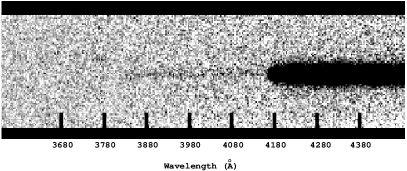
Figure 1: The two dimensional LRES spectrum, showing the position of the $z=3.572$ LL at $\sim 4170$ Å. The LL due to the $z=3.256$ system we are interested in can be seen at $\sim 3880$ Å.

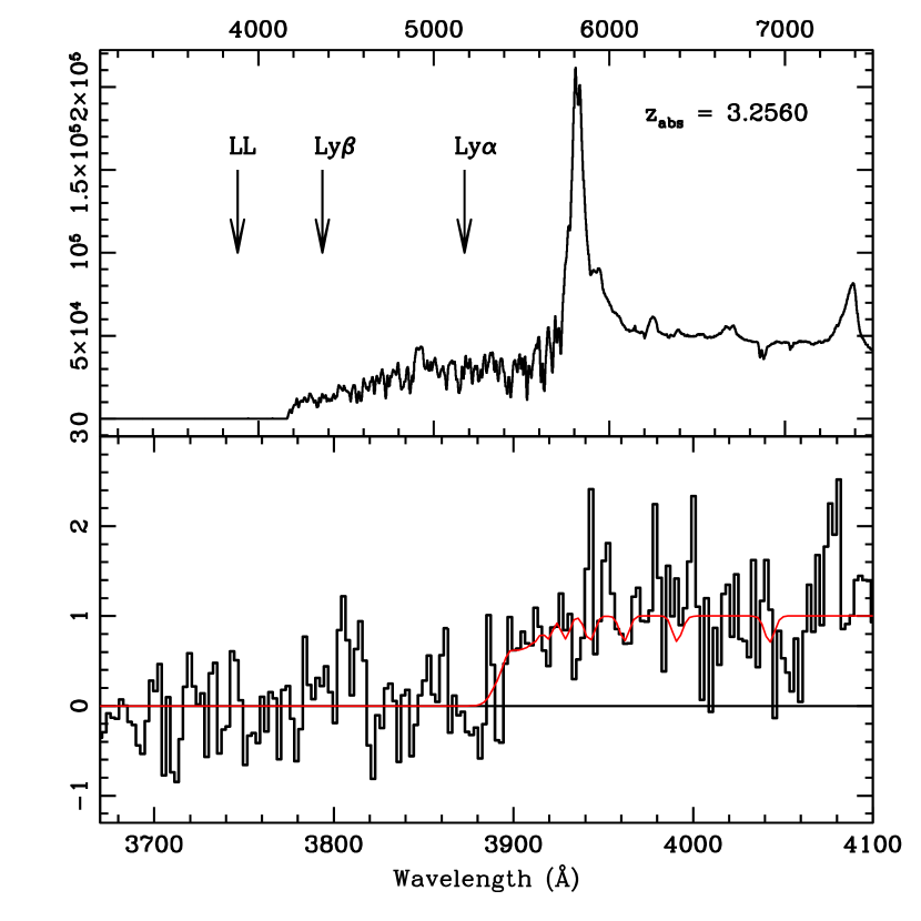
Figure 2: The entire LRES spectrum (above) and an expanded region of the spectrum showing the LL due to the $z=3.256$ absorber (below). The fit corresponding to model (2d) (see section 3.3) is shown in the expanded spectrum.

3 Analysis

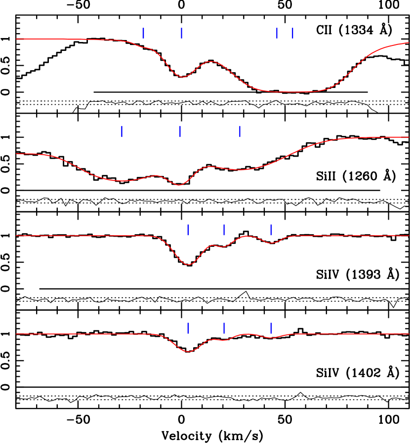
Figure 3: The C ii, Si ii and Si iv lines along with their best fitting models used to derive the parameters found in table 1. The velocity zero point is the redshift of the C ii line, $z=3.256009$. The histogram shows the data and the curves show the fitted model. The absorption lines away from the $v=0$ position in the top two panels are due to Ly$\alpha$ forest lines. The three components in the bottom two panels are all due to Si iv. The normalised residuals ($({\rm data}-{\rm model})/{\rm error}$) and their $1\sigma$ ranges are shown below each spectrum, offset from the zero level and scaled for clarity. Horizontal lines at zero flux show the fitting regions.

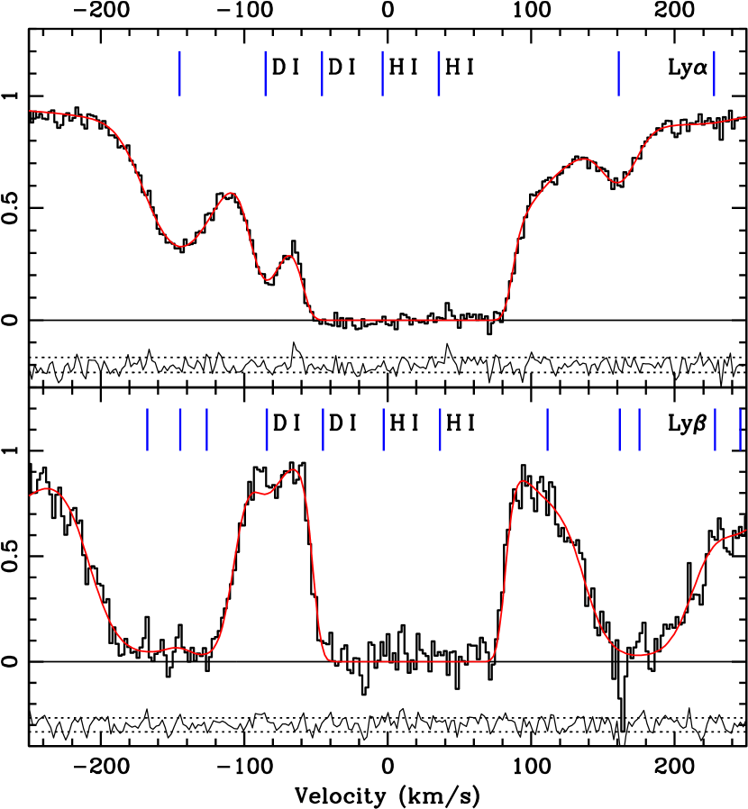
Figure 4: The Ly$\alpha$ and Ly$\beta$ lines, along with a fit to data. The fit corresponds to model (2d), a two H i component fit where the level of the continuum is allowed to vary above both the Ly$\alpha$ and Ly$\beta$ lines. The continuum over the Ly$\alpha$ line was generated using a 3rd order chebyshev polynomial. The velocity zero point is the redshift of the C ii line. The histogram shows the data and the narrow curve shows the fitted model. The normalised residuals are shown beneath each graph.

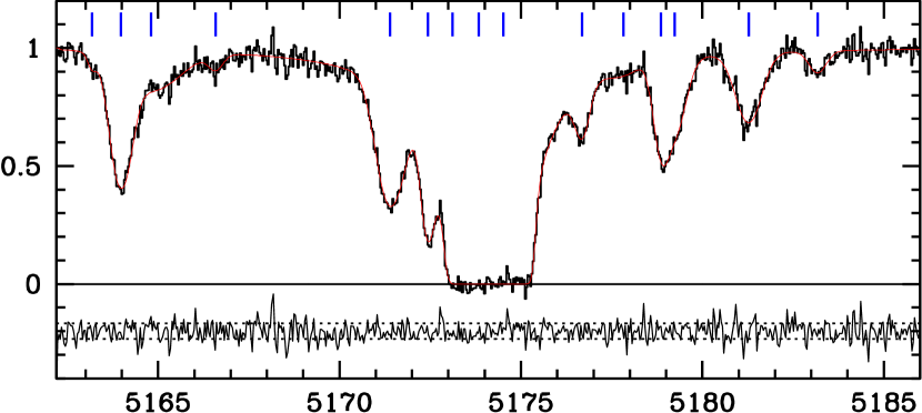
Figure 5: The Ly$\alpha$ line showing the damping wings and the best fitting model, model (2d). The histogram shows the data and the narrow curve shows the fitted model. The normalised residuals are shown below the spectrum.

We fit Voigt profiles to the relevant absorption lines using the program VPFIT. This uses a $\chi^{2}$ minimisation procedure to find the best fitting redshift, column density (cm^-2) and $b$ parameter (by definition, $b=\sqrt{2}\sigma$ where $\sigma$ is the Gaussian velocity dispersion) for each absorption line. The diagonals of the covariance matrix give the error estimates on each of the fitted parameters. These errors assume that the $\chi^{2}$ parameter space around the best fitting solution is parabolic, which is not always the case. In particular, if there are degeneracies in the fitted parameters, the $\chi^{2}$ parameter space needs to be explicitly explored to find the correct error ranges. For the majority of the transitions we fit in the $z=3.256$ system, the errors given by the covariance matrix are sufficiently accurate. However, to find the errors on the best fitting value of D/H, we do not use the errors given by VPFIT, but instead explicitly calculate $\chi^{2}$ as a function of D/H, as described in section 3.9.

3.1 Absorption lines present in the $z=3.256$ system

C ii (1334), Si ii (1260) and Si iv (1393 and 1402) (Fig. 3), H i Ly$\alpha$ and Ly$\beta$ (Fig. 4) transitions are present at $z=3.256$ in the HIRES spectrum. There is a narrow line in the blue wing of the H i Ly$\alpha$ line which we believe is D i. The $z=3.256$ Lyman limit (LL) is present in the LRES spectrum (Fig. 2). All higher order H i transitions are at wavelengths shorter than the LL due to the higher redshift absorber at $z=3.572$, and cannot be detected in our HIRES spectrum.

The HIRES spectrum covers the position of Si iii (1206.5) and Fe ii (1144), but they are blended with H i absorption in such a way that no useful constraints are possible.

Both the Si ii and C ii lines fall in the Ly$\alpha$ forest, where there is the danger that an H i forest line may be misidentified as a metal line. However, we are confident that we have correctly identified Si ii and C ii for two reasons. Firstly, their widths are much smaller than expected for the average Ly$\alpha$ forest H i line. Secondly, they fall within a few  kms^-1 of the expected redshift based on $z$(H i) and $z$(Si iv). Unfortunately, both Si ii and C ii lines are to some extent blended with H i Ly$\alpha$ absorption, which may be hiding weaker Si ii and C ii components.

The Si iv lines are at wavelengths longer than the quasar H i Ly$\alpha$ emission and so are not blended with forest lines.

The C ii and Si ii appear to be at the same redshift, $z$(C ii)$=3.256009\pm 0.000006$ and $z$(Si ii)$=3.256001\pm 0.000009$.

There are three Si iv components, one main component at $+3.4\pm 0.4$  kms^-1(redward) relative to the C ii/Si ii position, and two lower column density components at $+21.4\pm 0.7$  kms^-1 and $+43.4\pm 0.7$  kms^-1.

The metal line parameters and their errors are given in Table 1.

Table 1: The absorption line parameters and their errors, found using from the diagonals of the covariance matrix in VPFIT, for C ii, Si ii and the three Si iv components.

Ion	log($N$) (cm-2)	z	$b$ ( kms-1)
C ii	13.600 $\pm$ 0.045	3.256009 $\pm$ 0.000006	6.9 $\pm$ 0.7
Si ii	12.875 $\pm$ 0.093	3.256001 $\pm$ 0.000009	5.0 $\pm$ 1.4
Si iv	12.820 $\pm$ 0.011	3.256057 $\pm$ 0.000002	6.5 $\pm$ 0.3
Si iv	12.138 $\pm$ 0.039	3.256303 $\pm$ 0.000005	1.3 $\pm$ 1.3
Si iv	11.970 $\pm$ 0.036	3.256626 $\pm$ 0.000006	2.8 $\pm$ 1.3

3.2 H i column density

The $z=3.256$ Lyman limit is optically thick, so there is a lower limit on the total log $N$(H i) of $\sim 17.6$. There are also damping wings at the Ly$\alpha$ line, which further constrain $N$(H i) (Fig. 5). There might be another explanation for these damping wings; perhaps the continuum dips over the Ly$\alpha$ line, due to an emission line on either side of the Ly$\alpha$ line. However, composite QSO spectra [e.g. Vanden Berk et al. (2001)] display no emission lines associated with the quasar redshift at the relevant wavelengths to cause this apparent dip in the continuum. We believe our two estimates of the continuum, described below, adequately account for any uncertainty in the shape of the continuum.

3.3 Continuum placement

To generate the continuum we fitted regions that were apparently free from absorption around each absorption feature, with low order Chebyshev polynomials. The damping wings present in the H i Ly$\alpha$ line provide the best constraint on the total $N$(H i), but the derived $N$(H i) value is sensitive to the placement and shape of the continuum above the damping wings. To take this into account, we fitted two different continua above the Ly$\alpha$ line using 2nd and 3rd order Chebyshev polynomials. We also allow the continuum to vary above the Ly$\alpha$ and Ly$\beta$ lines by multiplying it by a parameter, initially set to $1$, which is allowed to vary during the $\chi^{2}$ minimisation. We use two independent parameters to vary the continuum level above the Ly$\alpha$ and Ly$\beta$ lines. An example of the typical fitted values and errors for the two continuum parameters is given in Table 2. For all our models, the fitted continua are within $5$% of our initial guess for the continuum.

3.4 H i velocity structure

We try to determine the velocity structure in two ways: firstly, by fitting the available H i transitions with as few components as needed to obtain an acceptable fit, and secondly, by looking at the metal lines to indicate the possible position of H i components. Ideally we would like to fit many higher order H i Lyman transitions to help determine the velocity structure, but only the Ly$\alpha$ and Ly$\beta$ lines are available.

A single H i component cannot satisfactorily fit both the Ly$\alpha$ and Ly$\beta$ lines, so at least two components are present.

We expect at least four hydrogen components, one at $z$(C ii/Si ii) and three corresponding to the Si iv component positions. However, we don’t know what H i column density is associated with each one. We expect the C ii and Si ii components to have a greater proportion of their associated H gas in the form of H i, as their ionization potentials are close to that of H i. Therefore, if there is no significant metallicity variation across the absorption complex, an H i component near $z$(C ii/Si ii) is likely to be the dominant component in the Ly$\alpha$ and Ly$\beta$ line.

Below we describe the velocity models we explored.

3.4.1 Model (1): two H i components, $z$(H i) tied to $z$(C ii)

We initially assemble a model using two H i components, with the redshift of the bluer component tied to the C ii redshift. In this fit we include D i components for both H i components. We tie the redshifts of corresponding D i and H i components together, and fit a single D/H to both components (we discuss this assumption in section 3.8). Since the redder D i component is heavily blended with the bluer H i component, we tie its $b$ parameter to the $b$ parameter of the corresponding H i component, assuming purely thermal broadening (this assumption has no effect on the final D/H value; see section 3.6). We fit the summed total of the H i column density of both components, instead of individually fitting the column densities of each component. We do this because while the column density in each component is not well constrained, the total log $N$(H i) is. This model does not fit the D i line in the Ly$\alpha$ line adequately. We can obtain an acceptable fit if we include very weak absorption from some unknown contaminating metal line near the D i position. However, this results in D/H $<0.6\times 10^{-5}$ ($1\sigma$ upper limit). This is smaller than even the lowest estimates of the interstellar medium D/H, $\sim 1.0\times 10^{-5}$ (Hébrard & Moos 2003).

3.4.2 Model (2): two H i components, $z$(H i) not tied to $z$(metals)

It is possible that the main H i component does not fall at exactly the same position as the C ii and Si ii lines. This could be due to several reasons: perhaps an error in the wavelength calibration of a few  kms^-1, or a gradient in the metallicity across the cloud. For this reason, we explore a model that does not tie the redshifts of the H i components to that of the metal lines. This model is identical to the model above, except it no longer ties the redshift of the bluer H i component to the C ii line. This model gives an acceptable fit to the data. The position of the bluer hydrogen component is $-3.5\pm 0.7$  kms^-1 relative to C ii. The redder H i component is at $+36\pm 4$  kms^-1.

3.4.3 Model (3): four H i components, $z$(H i) tied to $z$(metals)

We included four H i components, the redshift of each tied to a metal line component redshift (one corresponding to the C ii/Si ii position and one for each Si iv component). We include D i for all components where log $N$(H i)$>17.0$. This does not give a satisfactory fit to the data: the narrow D i line in the Ly$\alpha$ line in particular is very poorly fit. As in model (1), the fit could be improved by including very weak contaminating absorption near the D i position. Again, this gives a low D/H, $<0.5\times 10^{-5}$, much lower than the ISM D/H.

Model (2) gives the only acceptable fit to the data. Models (1) and (3) can give an acceptable fit, but we need to include an unidentified metal line blended with D i, and there is no other evidence that this is present. If we do include such a line, the measured D/H in this absorber is much smaller than the ISM D/H.

We split model (2) into four sub-models, using (2a) a 2nd order polynomial fixed continuum, (2b) a 3rd order polynomial fixed continuum, (2c) a 2nd order polynomial varying continuum and (2d) a 3rd order polynomial varying continuum.

Table 2: The best fitting parameters of the lines used to fit the Ly$\alpha$ and Ly$\beta$ lines and the LL of the $z=3.256$ absorber. The errors are those returned by VPFIT, calculated using the diagonals of the covariance matrix. The first two H i components in the table have associated D i lines which we included. We fitted the total column density of both these components - the column density entry next to the first H i component give the value of and error on the total column density of both H i components. The bottom two rows give the best fitting continuum parameters (which are multiplied by the initial guess for the continuum level) for the Ly$\alpha$ and Ly$\beta$ regions.

Ion	log$N$ (cm-2)	z	$b$ ( kms-1)
H i	18.255 $\pm$ 0.018 (total)	3.255959 $\pm$ 0.000008	15.8 $\pm$ 0.3
H i		3.256515 $\pm$ 0.000059	15.6 $\pm$ 1.3
D i	13.393 $\pm$ 0.069 (total)	3.255959 (tied to H i)	11.6 $\pm$ 0.9
D i		3.256515 (tied to H i)	11.1 (tied to H i)
H i	13.515 $\pm$ 0.014	3.253948 $\pm$ 0.000007	26.9 $\pm$ 0.8
H i	12.775 $\pm$ 0.030	3.258296 $\pm$ 0.000011	15.1 $\pm$ 1.3
H i	13.73 $\pm$ 0.18	2.589492 $\pm$ 0.000042	15.4 $\pm$ 3.3
H i	14.12 $\pm$ 0.083	2.588996 $\pm$ 0.000059	33.9 $\pm$ 3.4
H i	12.09 $\pm$ 0.17	3.259237 $\pm$ 0.000112	28.4 $\pm$ 14.0
H i	12.97 $\pm$ 0.34	3.260086 $\pm$ 0.000042	15.5 $\pm$ 3.3
H i	13.09 $\pm$ 0.26	3.260394 $\pm$ 0.000146	23.4 $\pm$ 6.4
H i	13.118 $\pm$ 0.014	3.262072 $\pm$ 0.000010	27.3 $\pm$ 1.0
H i	12.399 $\pm$ 0.054	3.263637 $\pm$ 0.000025	18.4 $\pm$ 2.7
H i	13.362 $\pm$ 0.036	3.247846 $\pm$ 0.000006	21.5 $\pm$ 1.0
H i	13.195 $\pm$ 0.073	3.248529 $\pm$ 0.000114	63.0 $\pm$ 8.7
H i	11.89 $\pm$ 0.23	3.247192 $\pm$ 0.000030	7.7 $\pm$ 4.6
H i	12.15 $\pm$ 0.11	3.249996 $\pm$ 0.000035	14.8 $\pm$ 4.1
H i	14.179 $\pm$ 0.031	2.593103 $\pm$ 0.000016	32.6 $\pm$ 3.2
H i	12.63 $\pm$ 0.38	2.592337 $\pm$ 0.000129	20.3 $\pm$ 13.8
H i	13.21 $\pm$ 0.11	2.593948 $\pm$ 0.000064	27.9 $\pm$ 5.9
H i	13.093 $\pm$ 0.094	2.587331 $\pm$ 0.000015	12.1 $\pm$ 2.5
H i	13.548 $\pm$ 0.038	2.587413 $\pm$ 0.000031	53.4 $\pm$ 5.5
H i	12.53 $\pm$ 0.10	2.586028 $\pm$ 0.000024	11.2 $\pm$ 3.4
cont(Ly$\alpha$)	1.0035 $\pm$ 0.0027
cont(Ly$\beta$)	0.983 $\pm$ 0.014

3.4.4 Two unresolved questions about the best-fitting model

The best fitting model seems to fall below the data at $-90$  kms^-1 in the Ly$\beta$ line (Fig. 4). There could be several reasons for this. It is possible that the apparent discrepancy is due to noise, or there may be a weak, narrow Ly$\alpha$ forest line near $-75$  kms^-1. However, such a line would need to have a width much smaller than the median width of forest lines. A metal line could have a narrow width, but the higher redshift system at $z=3.572$ does not have any metal lines which fall at this position. No other absorption systems were identified that could explain a metal line appearing at this position. Instead there may be a weak cosmic ray at this position that has not been completely removed. Two of the three 2D raw images combined to form the final spectrum show cosmic rays at the positions corresponding to $-75$ to $-95$  kms^-1 in the Ly$\beta$ line. We tentatively conclude that a noise spike is the cause of this discrepancy. We checked whether this discrepancy has a significant effect on the measured D/H by fitting the Ly$\alpha$, Ly$\beta$ lines and LL excluding the region from $-75$ to $-95$  kms^-1. We found that the best fitting D/H value and its error are almost unchanged, as the tightest constraint on $N$(D i) comes from the Ly$\alpha$ D i line.

We would expect the Si ii and C ii redshifts to be consistent with the redshift of the H i line associated with them. Instead we find that the Si ii/C ii position differs from the H i position by $3.5\pm 0.7$  kms^-1, or about $1.5$ pixels. It is possible that there are problems with the wavelength calibration. This is unlikely, however, given that the Si ii and C ii positions agree to within $1$ kms^-1, and that the typical wavelength accuracy of a polynomial fit to an arc exposure from HIRES is better than $0.5$  kms^-1. It is more likely that our velocity model is wrong in some way. The true velocity structure of the absorption complex will almost certainly be more complicated than our simple two component model. However, we note for all other velocity models that we considered, D/H was substantially lower ($<0.6\times 10^{-5}$) than the value that we quote for Model 2(b).

Both of these questions may be resolved by much higher S/N observations of this absorption system.

3.5 Ionization and metallicity

Figure 6: The ionization model generated using CLOUDY. The parameter $U$ is defined in section 3.5.

We have $N$(Si ii) and $N$(C ii) in a single gas cloud, and $N$(Si iv) in three other clouds. We use the program CLOUDY (Ferland 1997) to generate an ionization model for the absorption system. When generating the model, we assume that the bluest Si iv component, the Si ii and C ii component, and the bluest H i component are all associated with the same gas, even though they span $\sim 6$  kms^-1. We approximate the geometry of the cloud as a plane parallel slab illuminated by a distant point source and assume the proportion of metals to be solar. For calculating ionization fractions, the hydrogen particle density, $n_{H}$ and the incident radiation flux on the cloud, $J_{\nu}$ are degenerate. Instead of specifying either $n_{H}$ or $J_{\nu}$, we use the parameter $U$:

$$U=2\times 10^{-5}\frac{J_{912}/(10^{-21.5}\textrm{erg cm${}^{-2}$ s${}^{-1}$ sr${}^{-1}$})}{n_{H}/(1\rm{cm^{-3}})}$$

Here $J_{912}$ is the incident radiation at $912$ Å. We generate ionization models for a range of metallicities and $U$ values, using a Haardt-Madau ionizing radiation continuum at a redshift of $3.25$ (Haardt & Madau 1996). We have not explored the effect a different ionizing radiation continuum may have on the ionization fractions. $N$(Si ii) and $N$(Si iv) suggest that the system has a total metallicity [Si/H] $\sim-2.0$. $N$(C ii) is lower than expected for this [Si/H] which might indicate that C is under abundant compared to Si (see Fig. 6). This is unlikely to be due to differential dust depletion, since C has a lower condensation temperature than Si. We would expect Si, not C, to be under abundant if there is any depletion on to dust (Lu et al. 1996). However, an under abundance of C is consistent with metallicity measurements in metal poor stars and H ii regions, which find [C/O] $\sim-0.5$ (Akerman et al. 2004). Since both Si and O are $\alpha$-capture elements, it is reasonable to also expect [C/Si] $\sim-0.5$ when [Si/H] $=-2$ (Max Pettini, 2004, private communication).

With so few transitions we can only make broad generalisations about conditions in the cloud. We take a value of [Si/H] $-2.0$ with an error of $\sim 0.5$ dex, where this error is dominated by the uncertainty on $N$(H i) in the bluest H i component.

3.6 b parameter test

Figure 7: The $b$ parameter squared ( kms^-1)² versus the inverse ion mass (amu^-1). The dashed line is the least squares line of best fit to the Si ii, C ii, and H i points. D i is shown for comparison. The error bars in each case are calculated from the 1$\sigma$ errors given by VPFIT.

We can predict the $b$ parameter of the blue D i component from the $b$ parameters of the Si ii, C ii and H i lines. This is done by measuring the thermal line broadening, $b_{\rm{therm}}$, and turbulent broadening, $b_{\rm{turb}}$, by using the $b$ parameters from all available ions. If we assume the absorbing cloud has a thermal Maxwell-Boltzmann distribution and any turbulence can be described by a Gaussian velocity distribution, then the $b$ parameter for a particular ion will be given by

$$b_{\rm{ion}}^{2}=b_{\rm{therm}}^{2}+b_{\rm{turb}}^{2}.$$ (1)

Here $b_{\rm{therm}}^{2}=\frac{2kT}{m}$, where $T$ is the temperature of the gas cloud, $m$ is the mass of the absorbing ion and $k$ is Boltzmann’s constant. $b_{\rm{turb}}^{2}$ represents the Gaussian broadening due to small scale turbulence, and is the same for all ionic species. We plot $b^{2}$ against inverse ion mass in Fig. 7. Subject to the assumptions above, all the ions in the same cloud velocity space should lie on a straight line whose intercept gives $b_{\rm{turb}}$ and slope gives the cloud temperature. C ii, Si ii and H i all have relatively low ionization potentials (IP); 24.4, 16.3 and 13.6 eV, respectively. There is evidence from damped Ly$\alpha$ absorbers that even ‘intermediate’ IP ions, such as Al iii (IP 28.4 eV), have a similar velocity structure to lower IP ions (Wolfe & Prochaska 2000). Thus we assume that the Si ii and C ii lines arise in the same gas as the H i  and fit a least squares line of best fit to these three points. This is shown as the dashed line in Fig. 7. The D i point is plotted with its $1\sigma$ error bars as given by VPFIT. We find a temperature of $1.35\pm 0.08\times 10^{4}$K and a turbulent broadening of $5.0\pm 0.8$ kms^-1. These values suggest a $b$ parameter for the blue D i component of $11.7$  kms^-1. This is consistent with our fitted $b$(D i) of $11.6\pm 0.9$  kms^-1 for the blue D i component.

There is no way to measure the $b$ parameter of the red D i component, since it is heavily blended with the H i blue component. We also cannot predict what $b$(D i) will be using the method above, since we do not have any low ionization metal lines corresponding to the red H i component. In our velocity models we explored the maximum and minimum $b$(D i) values, corresponding to purely thermal [$b$(D i)$=1/\sqrt{2}\ b$(H i)] and purely turbulent [$b$(D i) $=b$(H i)] broadening. The measured D/H is not affected by which broadening we assume. Thus we arbitrarily choose pure thermal broadening, assuming that the the conditions in the red component are similar to the blue component.

3.7 Are we seeing deuterium?

We expect we are seeing D, for three reasons. The line we have identified as D i occurs near the expected position for D i, given the position of the main H i absoprtion and the position of the Si ii and C ii lines. The $b$ parameter of the D i line is consistent with that expected for D i based on the fitted $b$ parameters of the H i component and the Si ii and C ii lines. Finally, the line has a width substantially narrower than the median for forest lines, which means it is unlikely to be an H i Ly$\alpha$ forest line. A metal line from another absorption system could have a line width this narrow, but we know of no other absorption systems towards this quasar which have metal lines that fall at the position of the D i line. These arguments all apply only to the bluer D i component. We cannot independently measure the position, $b$ parameter or column density of the the redder D i component. However, we assume that D/H is the same in both components for the reasons given in section 3.8.

3.8 The validity of our assumption of constant D/H across different components

We assume in our models that D/H is the same for all components showing D i. D is destroyed in star formation, so if the components have different metallicities, it is conceivable that they will also have different D/H values. Unfortunately, we cannot directly measure the metallicity of individual components due to the Ly$\alpha$ forest contamination around the Si ii and C ii lines. However, we believe that even if the metallicity is significantly different in different components, D/H will still be very similar. Even in systems where the metallicity has been found to vary considerable between components in the same absorption system (e.g. Kirkman et al. 2003; Burles & Tytler 1998a), the difference is rarely more than $\sim 1.0$ dex. Theoretical models (Fields 1996; Prantzos & Ishimaru 2001) predict that D/H remains roughly constant with metallicity until metallicities approaching $1/5$ solar are reached. Since [Si/H] $\sim-2.0$ for this entire absorption complex (see section 3.5), we expect D/H in this absorber to be very close to the primordial value. Even if there are components with [Si/H] as high as $\sim-1.0$ present, we don’t expect their D/H to be significantly lower than that of any lower metallicity components.

3.9 D/H in the z=3.256 absorber

Figure 8: $\chi^{2}$ vs D/H plots. The horizontal lines show the $68.3$% and $95.4$% confidence levels. The upper graphs are for models (2c) and (2d), where the continuum level is allowed to vary during the fit. The lower models are (2a) and (2b), where the continuum levels are fixed. The plots on the left use models with a 2nd order continuum fit over the Ly$\alpha$ line, the plots on the right use a 3rd order continuum.

We have the values of $N$(H i) and $N$(D i) and their errors for models (2a) - (2d), but we prefer to use an alternate method to find D/H in this absorber. Only two small regions constrain $N$(D i), and the errors on $N$(D i) are relatively large. As we saw in Crighton et al. (2003), when the errors given by VPFIT are large, it is often a sign that the $\chi^{2}$ parameter space around the best fitting solution is not symmetrical. In this case the $\chi^{2}$ space should be explored explicitly to find the correct error ranges.

We have generated a list of $\chi^{2}$ values as a function of D/H. For each value of D/H, we fix D/H and fit the Ly$\alpha$, Ly$\beta$ lines and the LL, varying all other parameters to minimise $\chi^{2}$. In this case we do not fit the the total $N$(H i) and $N$(D i), since we are not interested in the errors on individual parameters, just the total $\chi^{2}$ value. In this fit we tie the redshifts of each D i line to its corresponding H i line. We also tie the $b$ parameter of the red D i component to its correponding H i component, assuming thermal broadening, as discussed in section 3.6.

We calculate one of these graphs for an appropriate range of D/H values for each model, (2a) - (2d) (Fig. 8). The distribution of $\Delta\chi^{2}\equiv\chi^{2}-\chi^{2}_{\rm{min}}$ for each graph is the same as that of a $\chi^{2}$ distribution with a number of degrees of freedom equal to the number of fixed parameters (in this case, one - D/H). Here $\chi^{2}_{\rm{min}}$ is the smallest value of $\chi^{2}$ for a particular graph. For each point on each graph, we are fitting $990$ data points with $\sim 47$ parameters, giving $\sim 943$ degrees of freedom. The typical reduced $\chi^{2}$ for our best fitting models is $1.2$.

D/H is more tightly constrained in the cases without a floating continuum level, which is expected as there are fewer free parameters. The 3rd order continuum allows a better fit to the data than the 2nd, and is consistent with a larger D/H value. The predicted $68.3$% range for D/H for the 3rd order continuum models (2b and 2d) is $1.6^{+0.25}_{-0.30}\times 10^{-5}$, with a $95.4$% range of $1.6^{+0.5}_{-0.4}\times 10^{-5}$. The D/H ranges for the 2nd order continuum models are lower, $\sim 1.45\pm 0.2\times 10^{-5}$. Model (2d), which takes the uncertainty in the continuum level [and any effect that may have on the uncertainty in the $N$(H i) value] into account, gives the best estimate of D/H in this absorber. It is worth noting that these error ranges are consistent with the ranges for D/H that would be derived by using the VPFIT best fitting values and errors given in Table. 2.

4 Comparison with D/H measured in other QSO absorbers

Figure 9: D/H measurements as a function of log$N$(H i) in the absorber where the measurement was made. The filled circle is the D/H value from this paper. The hashed region is the CMB + standard BBN prediction for D/H from Coc et al. (2004). References for the other D/H measurements are given in section 4.

In this section we compare other D/H detections with our own detection, and the predicted D/H value from CMB and standard BBN. There are many upper limits on D/H in QSO absorbers that are much higher than the CMB predicted D/H. Examples of such systems are towards Q0014+813 (Carswell et al. 1994; Rugers & Hogan 1996a, b; Burles et al. 1999), Q0420-388 (Carswell et al. 1996), BR 1202-0725 (Wampler et al. 1996), PG 1718-4801 (Webb et al. 1997; Tytler et al. 1999; Kirkman et al. 2001; Crighton et al. 2003) and Q0130-4021 (Kirkman et al. 2000). We do not include these in our comparison, since they are clearly consistent with the predicted D/H value.

We now describe six D/H detections in QSO absorbers, five of which we include in our comparison. We exclude one of the detections, towards Q0347-3819, for the reasons outlined below in section 4.5.

4.1 $z=3.572$ towards PKS1937-1009

Burles & Tytler (1998a) have presented the most comprehensive analysis of this system. Absorption attributed to D i is observed in two transitions. The measured $b$(D i) matches the predicted $b$ found using the Si ii, C ii and H i $b$ parameters. This is a grey LL system. $N$(H i) was measured using the drop in flux at the LL and initially estimated by Tytler et al. (1996) as log $N$(H i) $=17.94\pm 0.05$. This was revised in Burles & Tytler (1997) to $17.86\pm 0.02$ after Wampler (1996) and Songaila et al. (1997) pointed out that the continuum level of Tytler et al. was too high. The final D/H value from Burles & Tytler (1998a) is $(3.3\pm 0.3)\times 10^{-5}$.

4.2 $z=2.504$ towards 1009+2956

This system was analysed by Burles & Tytler (1998b). It has a grey LL and log $N$(H i) $=17.39\pm 0.06$, measured using the drop in flux at the LL. D i is seen in only a single transition. The authors believe it is likely some contamination is present, so the D i parameters are less certain than in other systems. As in our paper, the authors assume a constant D/H across the entire absorption complex. D/H $=(4.0^{+0.6}_{-0.7})\times 10^{-5}$.

4.3 $z=2.536$ towards HS0105+1619

O’Meara et al. (2001) analysed this system and found that $b$(H i) is very small ($\sim 14$  kms^-1), meaning that each D i line is clearly separated from the nearby H i absorption. Consequently $b$(D i) and $N$(D i) can be measured independently of the H i absorption parameters. log $N$(H i) $=19.422\pm 0.009$ is determined by the damping wings in the Ly$\alpha$ line, and D i is seen in five transitions. A relatively precise D/H can be derived: D/H $=(2.54\pm{0.23})\times 10^{-5}$.

4.4 $z=2.076$ towards QSO 2206-199

Pettini & Bowen (2001) find a very low $b$(H i) ($\sim 14$  kms^-1) and an extremely simple velocity structure (apparently a single H i component). This allows a D/H measurement despite the relatively low S/N of their HST spectra. Two Lyman transitions can be used to constrain $N$(D i). log $N$(H i) $=20.436\pm 0.008$ is measured using the damping wings of the H i Ly$\alpha$ line. D/H $=(1.65\pm 0.35)\times 10^{-5}$.

4.5 $z=3.025$ towards Q0347-3819

This system was initially analysed by D’Odorico et al. (2001), who found D/H $=(2.24\pm 0.67)\times 10^{-5}$. It was subsequently re-analysed by Levshakov et al. (2002), who found D/H $=(3.75\pm 0.25)\times 10^{-5}$. log $N$(H i) $=20.626\pm 0.005$ is measured using the damping wings in the Ly$\alpha$ line. Levshakov et al.’s result is different because they assume the main component in H i has a similar $z$ and $b$ to that of H₂, also observed in this absorber. The D i lines are heavily blended with H i and neither $b$(H i) nor $b$(D i) can be measured directly. The D/H value derived is dependent on the assumed velocity structure, as shown by the different results of D’Odorico et al. and Levshakov et al. The Si iv and C iv transitions for this absorber in Prochaska & Wolfe (1999) show components at $\sim-60$  kms^-1 (on the scale in Levshakov et al.’s Fig. 10), which may have associated H i absorption that could affect the derived D/H. We suspect that the range of D/H values allowed in this absorber is significantly larger than that quoted by Levshakov et al. (2002). If we were to include this result, we would choose a conservative $1\sigma$ error range of $(1.57-4.00)\times 10^{-5}$. Since this range is at least a factor of $2$ greater than the other D/H error ranges, we exclude this value from our comparison of D/H values below.

4.6 $z=2.526$ towards Q1243+3047

Kirkman et al. (2003) analysed this system. D i is seen in five transitions, but blended with H i. $N$(H i) is measured using the damping wings at Ly$\alpha$. This is complicated by the Ly$\alpha$ lying close to the quasar H i Ly$\alpha$ emission, where the continuum is steep and difficult to determine. The authors generate many continua based on ‘anchor’ points in the spectrum which they assume are free from forest absorption. They use these to find a robust estimate for log $N$(H i) $=19.73\pm 0.04$. The fitted $b$(D i) is marginally consistent with the predicted value from $b$(H i) and $b$(O i). D/H $=(2.42^{+0.35}_{-0.25})\times 10^{-5}$.

All of these D/H measurements are in absorbers with metallicities of [Si/H] $<-1$, and so no significant D astration should have taken place. Thus we might expect all of these values, along with the D/H value from this paper, to be consistent with a single, primordial D/H. To test this, we fitted the five adopted D/H values above together with the value in this paper to a single D/H value. Where there are not symmetrical errors around the D/H values, we force them to be symmetrical by increasing the smaller error to match the larger error. We find D/H $=(2.40\pm 0.3)\times 10^{-5}$, which is consistent with the predicted D/H from CMB and standard BBN, $(2.60^{+0.19}_{-0.17})\times 10^{-5}$ (Coc et al. 2004). The value of the total $\chi^{2}$ for the fit is $25.95$ for five degrees of freedom. The chance of exceeding this $\chi^{2}$ value by chance is less than 0.01 %. Thus, taken at face value, the measurements are not consistent with a single D/H; but with so few measurements this may just be a result of small number statistics. Kirkman et al. (2003) argue that the inconsistency is probably due to underestimated systematic errors - indeed, if we artificially double all the errors of the D/H values, the total $\chi^{2}=6.5$ and the inconsistency disappears. However, we note that the statistical errors on each D/H result were arrived at only after careful consideration of systematic errors. This highlights the need for further D/H measurements to determine whether the scatter in D/H is real.

4.7 Correlation between D/H and $N$(H i)

Pettini & Bowen (2001) and Kirkman et al. (2003) note that there appears to be a trend of decreasing D/H with increasing $N$(H i). Our result does not follow this trend, and has a much lower D/H value than either of the two other low $N$(H i) systems towards PKS1937-1009 and 1009+2956 (Fig. 9). We are not sure of the reason for this difference. As Pettini & Bowen (2001) commented, it is interesting that the two systems with the highest D/H values are both grey LL systems, where the total $N$(H i) was measured using the drop in flux at the LL. In all the other D/H systems, including the one in this paper, the dominant constraint on the $N$(H i) value is from the damping wings of the Ly$\alpha$ or Ly$\beta$ lines. At first glance this might suggest a systematic error in measuring $N$(H i) could explain the difference between our D/H and the grey LL D/H values, although previous authors’ analyses of systematics affecting $N$(H i) in both grey LL and higher $N$(H i) systems have been very thorough.

5 Discussion

We have identified a new Lyman limit absorption system towards PKS1937-1009, with log$N$(H i) $=18.25\pm 0.02$ at $z=3.256$. The Ly$\alpha$ and Ly$\beta$ transitions are suitable for measuring D/H, and we find a $68.3$% range for D/H of $1.6^{+0.25}_{-0.30}\times 10^{-5}$, and a $95.4$% range of $1.6^{+0.5}_{-0.4}\times 10^{-5}$.

The metallicity of the cloud where D/H was measured is low, [Si/H] $=-2.0\pm 0.5$. At this metallicity we expect that the D/H value will be primordial.

This value disagrees at the $99.4$% level with the predicted D/H value using the $\Omega_{b}$ calculated from the WMAP cosmic background radiation measurements, $2.60^{+0.19}_{-0.17}\times 10^{-5}$ (Coc et al. 2004), and it exacerbates the scatter in D/H measurements around the mean D/H value. It is consistent with the D/H values measured in the ISM using FUSE, (e.g. Hébrard & Moos 2003). However, it is not consistent with the idea of a single primordial D/H value which stays constant until the metallicity reaches $\sim 1/10$ solar, then begins to drop off, reaching the ISM D/H at solar metallicity. Some early mechanism for D astration may be the cause for the scatter in D/H values (Fields et al. 2001), although in this case we would expect to see a correlation between D/H and [Si/H], which is not observed.

Other authors (Pettini & Bowen 2001; Kirkman et al. 2003) note that there is a trend of decreasing D/H with increasing $N$(H i) of the absorbers in which they are measured. The D/H value in this paper does not follow this trend, suggesting that the trend is not real and only due to the low number of D/H measurements.

We would like to thank Antoinette Songaila for making the Keck data used in this analysis available and Max Pettini for his helpful correspondence. We also thank the anonymous referee for their constructive comments that helped improve the paper. AOG and AFS acknowledge support from the Generalitat Valenciana ACyT project GRUPOS03/170, and Spanish MCYT projects AYA2002-03326 and AYA2003-08739-C02-01.

References

- Akerman et al. (2004) Akerman C. J., Carigi L., Nissen P. E., Pettini M., Asplund M., 2004, A&A, 414, 931
- Barger et al. (2003) Barger V., Kneller J. P., Langacker P., Marfatia D., Steigman G., 2003, Physics Letters B, 569, 123
- Burles et al. (1999) Burles S., Kirkman D., Tytler D., 1999, ApJ, 519, 18
- Burles & Tytler (1997) Burles S., Tytler D., 1997, AJ, 114, 1330
- Burles & Tytler (1998a) Burles S., Tytler D., 1998a, ApJ, 499, 699
- Burles & Tytler (1998b) Burles S., Tytler D., 1998b, ApJ, 507, 732
- Carswell et al. (1994) Carswell R. F., Rauch M., Weymann R. J., Cooke A. J., Webb J. K., 1994, MNRAS, 268, L1+
- Carswell et al. (1996) Carswell R. F., Webb J. K., Lanzetta K. M., Baldwin J. A., Cooke A. J., Williger G. M., Rauch M., Irwin M. J., Robertson J. G., Shaver P. A., 1996, MNRAS, 278, 506
- Coc et al. (2004) Coc A., Vangioni-Flam E., Descouvemont P., Adahchour A., Angulo C., 2004, ApJ, 600, 544
- Crighton et al. (2003) Crighton N. H. M., Webb J. K., Carswell R. F., Lanzetta K. M., 2003, MNRAS, 345, 243
- Cyburt et al. (2003) Cyburt R. H., Fields B. D., Olive K. A., 2003, Physics Letters B, 567, 227
- Dmitriev et al. (2004) Dmitriev V. F., Flambaum V. V., Webb J. K., 2004, Phys. Rev. D, 69, 063506
- D’Odorico et al. (2001) D’Odorico S., Dessauges-Zavadsky M., Molaro P., 2001, A&A, 368, L21
- Epstein et al. (1974) Epstein R. I., Lattimer J. M., Schramm D. N., 1974, Nat, 263, 198
- Ferland (1997) Ferland G., 1997, Hazy, a Brief Introduction to Cloudy. University of Kentucky, Department of Physics and Astronomy Internal Report
- Fields (1996) Fields B. D., 1996, ApJ, 456, 478
- Fields et al. (2001) Fields B. D., Olive K. A., Silk J., Cassé M., Vangioni-Flam E., 2001, ApJ, 563, 653
- Hébrard & Moos (2003) Hébrard G., Moos H. W., 2003, ApJ, 599, 297
- Haardt & Madau (1996) Haardt F., Madau P., 1996, ApJ, 461, 20
- Ichikawa & Kawasaki (2004) Ichikawa K., Kawasaki M., 2004, Phys. Rev. D, 69, 123506
- Kirkman et al. (2000) Kirkman D., Tytler D., Burles S., Lubin D., O’Meara J. M., 2000, ApJ, 529, 655
- Kirkman et al. (2001) Kirkman D., Tytler D., O’Meara J. M., Burles S., Lubin D., Suzuki N., Carswell R. F., Turner M. S., Wampler E. J., 2001, ApJ, 559, 23
- Kirkman et al. (2003) Kirkman D., Tytler D., Suzuki N., O’Meara J. M., Lubin D., 2003, ApJS, 149, 1
- Lanzetta et al. (1991) Lanzetta K. M., McMahon R. G., Wolfe A. M., Turnshek D. A., Hazard C., Lu L., 1991, ApJS, 77, 1
- Levshakov et al. (2002) Levshakov S. A., Dessauges-Zavadsky M., D’Odorico S., Molaro P., 2002, ApJ, 565, 696
- Lu et al. (1996) Lu L., Sargent W. L. W., Barlow T. A., Churchill C. W., Vogt S. S., 1996, ApJS, 107, 475
- O’Meara et al. (2001) O’Meara J. M., Tytler D., Kirkman D., Suzuki N., Prochaska J. X., Lubin D., Wolfe A. M., 2001, ApJ, 552, 718
- Pettini & Bowen (2001) Pettini M., Bowen D. V., 2001, ApJ, 560, 41
- Prantzos & Ishimaru (2001) Prantzos N., Ishimaru Y., 2001, A&A, 376, 751
- Prochaska & Wolfe (1999) Prochaska J. X., Wolfe A. M., 1999, ApJS, 121, 369
- Rugers & Hogan (1996a) Rugers M., Hogan C. J., 1996a, ApJ, 459, L1+
- Rugers & Hogan (1996b) Rugers M., Hogan C. J., 1996b, AJ, 111, 2135
- Sembach et al. (2004) Sembach K. R., Wakker B. P., Tripp T. M., Richter P., Kruk J. W., Blair W. P., Moos H. W., Savage B. D., Shull J. M., York D. G., Sonneborn G., Hébrard G., Ferlet R., Vidal-Madjar A., Friedman S. D., Jenkins E. B., 2004, ApJS, 150, 387
- Songaila et al. (1997) Songaila A., Wampler E. J., Cowie L. L., 1997, Nat, 385, 137
- Spergel et al. (2003) Spergel D. N., Verde L., Peiris H. V., Komatsu E., Nolta M. R., Bennett C. L., Halpern M., Hinshaw G., Jarosik N., Kogut A., Limon M., Meyer S. S., Page L., Tucker G. S., Weiland J. L., Wollack E., Wright E. L., 2003, ApJS, 148, 175
- Tytler et al. (1999) Tytler D., Burles S., Lu L., Fan X., Wolfe A., Savage B. D., 1999, AJ, 117, 63
- Tytler et al. (1996) Tytler D., Fan X.-M., Burles S., 1996, Nat, 381, 207
- Vanden Berk et al. (2001) Vanden Berk D. E., Richards G. T., Bauer A., Strauss M. A., Schneider D. P., Heckman T. M., York D. G., Hall P. B., Fan X., 2001, AJ, 122, 549
- Wampler (1996) Wampler E. J., 1996, Nat, 383, 308
- Wampler et al. (1996) Wampler E. J., Williger G. M., Baldwin J. A., Carswell R. F., Hazard C., McMahon R. G., 1996, A&A, 316, 33
- Webb et al. (1997) Webb J. K., Carswell R. F., Lanzetta K. M., Ferlet R., Lemoine M., Vidal-Madjar A., Bowen D. V., 1997, Nat, 388, 250
- Wolfe & Prochaska (2000) Wolfe A. M., Prochaska J. X., 2000, ApJ, 545, 603