X-ray aurora in neutron star magnetospheres

Abstract

The discovery of quasi-periodic oscillations (QPOs) in low-mass X-ray binaries (LMXBs) has been reported and discussed in recent studies in theoretical and observational astrophysics. The Rossi X-Ray Timing Explorer has observed oscillations in the X-ray flux of about 20 accreting neutron stars. These oscillations are very strong and remarkably coherent. Their frequencies range from $\sim 10$ Hz to $\sim 1200$ Hz and correspond to dynamical time scales at radii of a few tens of kilometers, and are possibly closely related to the Keplerian orbital frequency of matter at the inner disk. Almost all sources have also shown twin peaks QPOs in the kHz part of the X-ray spectrum, and both peaks change frequencies together.

Bearing in mind these facts, several models explain the observed frequencies by the oscillation modes of an accretion disk. In the beat-frequency interpretation, the upper kHz QPOs are associated with the Keplerian frequency of the accreting gas flowing around a weakly magnetized neutron star ($B\sim 10^{7}-10^{10}$ G) at some preferred orbital radius around the star, while the lower kHz QPOs result from the beat between the upper kHz QPO and the spin frequency of the neutron star. In the relativistic precession model, while the upper kHz QPO is still the orbital frequency of matter at some radius in the disk, the lower kHz QPOs are considered as general relativistic precession modes of a free particle orbit at that radius.

In this study we propose a new generic model for QPOs based on oscillation modes of neutron star magnetospheres. We argue that the interaction of the accretion disk with the magnetosphere can excite resonant shear Alfvén waves in a region of enhanced density gradients. We demonstrate that depending on the distance of this enhanced density region from the star and the magnetic field strength, the frequency of the field line resonance can range from several Hz (weaker field, farther from star), to approximately kHz frequencies (stronger field, $\sim 6-10$ star radii from the star). We show that such oscillations are able to significantly modulate inflow of matter from the high density region toward the star surface, and possibly produce the observed X-ray spectrum. In addition, we show that the observed $2:3$ frequency ratio of QPOs is a natural result of our model.

1 introduction

Recent years have seen a surge in interest in studies of accreting neutron stars and black holes. One reason is that these objects provide a very unique window to a deeper understanding of the physics of strong gravity and dense matter. The complicated structure of these stellar objects, including strong gravity, gravitationally-captured plasma accretion, rapid rotation, bursting in accreted materials, thermal X-ray emission, and several other features makes a most fascinating object for both theoretical and observational investigations. One of the most interesting features of these objects is the interaction of accreting plasma with the stellar magnetic field. Matter is transferred from a normal donor star to the compact object. MHD models of the infalling plasma and the neutron star magnetosphere allow a relatively simple first approach to an understanding of plasma flow and the configuration of the magnetosphere around a neutron star.

Research on plasma accretion by magnetic neutron stars began in the early 1970s with the discovery of periodic oscillations in X-ray fluxes of the stars Cen X-3 (Giacconi et al., 1971; Schreier et al., 1972) and Her X-1 (Tananbaum et al., 1972). Interest in these systems rose about two decades ago, after the first observation of quasi-periodic oscillations (QPOs) in the persistent X-ray fluxes of the luminous X-ray sources (van der Klis et al., 1985; Hasinger et al., 1986; Middleditch & Priedhorsky, 1986). These oscillations are detected both in low and high frequencies with frequencies ranging from $\sim 1$ to $\sim 100$ Hz and from $\sim 300$ to $\sim 1200$ Hz, respectively. The Rossi X-Ray Timing Explorer (RXTE) has observed persistent X-ray emissions about 20 accreting neutron stars in low-mass X-ray binaries (LMXBs). Generally, three different millisecond phenomena have now been observed in X-ray binaries: the twin kilohertz quasi-periodic oscillations (kHz QPOs), the burst oscillations, and the spin frequency of the accreting, low-magnetic field, neutron star. These kilohertz frequencies are the highest frequency oscillations ever seen in any astrophysical object, and are now widely interpreted as due to orbital motion in the inner accretion flow. The oscillations sometimes have one spectral peak. In most sources, however, the X-ray spectrum shows two simultaneous kHz peaks with a roughly constant peak separation, moving up and down together in time as a function of photon count rate. In this work, we focus on the Hz-kHz QPOs.

The burst oscillations with frequencies in the $300-600$ Hz range have been observed in a number of the X-rays sources, usually during a type I X-ray burst due to a thermonuclear runaway in the accreted matter on the neutron star surface. Furthermore, the frequency of the burst oscillation increases by $1-2$ Hz during the burst tail, converging in time to a stable frequency at the neutron star spin frequency. It is believed that the burst oscillations arise due to a hot spot or spots in an atmospheric layer of the neutron star. This has been explained by a decoupling of the atmospheric layer from the star and expansion by $5-50$ m during the X-ray burst, while its angular momentum remains constant. Therefore, during the burst tail, the frequency increases due to spin-up of the atmosphere as it re-contracts. The asymptotic frequency corresponds to a fully re-contracted atmosphere and is the closest to the true neutron star spin frequency (see the recent review by Bildsten & Strohmayer (2003)). In a few sources, however, a rather large frequency drift, $\sim 5-10$ Hz, is observed. This drift is not consistent with the above model ( see Rezania & Karmand (2003) for more details).

Although there are some detailed differences in different types of X-ray sources, the observed QPOs in all sources are remarkably similar, both in frequency and peak separation. (Six of the 20 known sources are originally identified as “Z” sources and the rest are known as “atoll” sources, see table 1. For more information about the atoll and Z sources, see van der Klis (2000).) Such a similarity shows that QPOs should depend on general characteristics of the X-ray sources which are common to all systems. In other words, the QPO can be regarded as a generic feature of the accreting neutron star.

In the accretion disk of accreting binaries the material from the donor star moves around the compact star in near-Keplerian orbits. Depending on the binary separation, the disk radius varies from $10^{5}$ to $10^{7}$ km. Although there is still no certainty about the flow geometry in the inner emitting region, the extension of a part of the flow down into the emitting region in the form of a Keplerian disk is the basic assumption of most proposed models for accretion of matter onto low magnetic field neutron stars (see for example Miller et al. (1998)). Due to the interaction with the magnetic field of the star, radiation drag, and relativistic effects, the flow will be terminated at a radius $r_{\rm in}$, the innermost stable orbital radius that is larger than radius of the compact star $R_{s}$. Within $r_{in}$ matter may leave the disk and so the flow is no longer Keplerian. Remarkably, the characteristic dynamical time scale for materials moving near the compact object is comparable with the observed millisecond X-ray variability, ie. $\tau_{\rm dyn}=(r^{3}/GM)^{1/2}\sim 2~{}{\rm ms}~{}(r/100{\rm km})^{3/2}(1.4M_{\odot}/M)^{1/2}$. Such a natural periodicity is the foundation of most models for the observed QPOs. We will discuss these models in the next section.

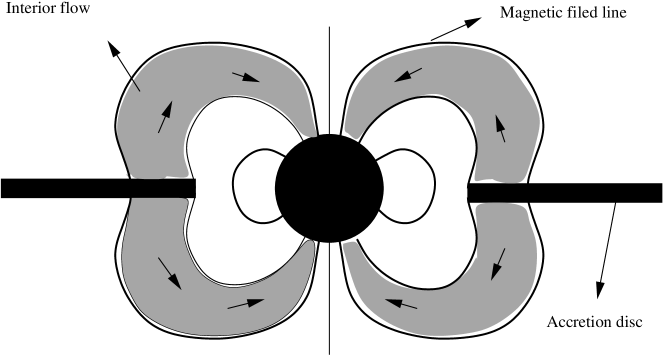
Figure 1: Side view of the magnetic field and accretion disk in accreting neutron stars. The neutron star’s strong gravity causes a very high velocity flow toward the magnetosphere. As a result, the magnetosphere is pushed inward in the disk plane but balloons outward in direction away from the disk plane. Some of the plasma may leave the disk and flow along the field lines.

Another common feature in accreting binaries is the interaction of the accretion disk with neutron star’s magnetosphere. In all sources, matters transfer from a normal donor star to the compact object. This matter is accelerated by the gravitational pull of the compact object and hits the magnetosphere of the star with a sonic/supersonic speed. The MHD interaction of the infalling plasma with the neutron star magnetosphere, will alter not only the plasma flow toward the surface of the star, as assumed by current QPO models, but also the structure of the star’s magnetosphere. The magnetic field of the neutron star is distorted inward by the infalling plasma of the Keplerian accretion flow. Since the gravity of the star confines the inward flow to a small solid angle $\sim 10^{-2}$ ster, the magnetic field of the star will be more compressed in the disk plane than in other areas, see Fig. 1. Furthermore, in a more realistic picture, one would expect that the highly accelerated plasma due to the infall process would be able to penetrate through the magnetic field lines. Such materials will be trapped by the magnetic field lines and produce enhanced density regions within the magnetosphere. However, due to their initial velocities, they move along the field lines, finally hit the star surface at the magnetic poles and produce the observed X-ray fluxes (Fig. 1). See Ghosh et al. (1977) for more detail.

Besides modifying the geometry of magnetosphere, the compressional action of the accretion flow can excite some perturbations in the enhanced density region. This can be understood by noting this fact that the inward motion of the accretion flow will be halted by the outward magnetic pressure at a certain distance from the star, the Alfvén radius (Ghosh et al., 1977). In other words, the accretion flow pushes the stellar magnetic field toward the star until the inward pressure of the infalling plasma $\rho v_{r}^{2}/2$ balances with the outward magnetic pressure $B_{p}^{2}/8\pi$. Here $\rho$ and $v_{r}$ are the density and radial velocity of the infalling matter and $B_{p}$ is the poloidal magnetic field at the disk plane. Therefore, any instability in the disk at the Alfvén radius would disturb such quasi-equilibrium configuration as well as the structure of magnetosphere. As an example, the interaction of the solar wind with earth magnetosphere excites resonant shear Alfvén waves, or field line resonances (FLRs), along the magnetic field lines (Samson, 1991). As a result, one might expect that such Alfvén waves can be excited by the compressive accreting plasma in the magnetosphere of an accreting neutron star with the accretion flow playing the role of the solar wind.

The plan of this paper is as follow: In section 2 we discuss some of the current models for the observed QPOs. Specifically, we will review the two models, the sonic-point beat frequency model and the relativistic precession model, in more detail. We outline an occurrence of the resonant coupling in a magnetized plasma in section 3. Specifically, we review the excitation of shear Alfvén waves by studying linear perturbations in MHD. Next, the occurrence of field line resonances (FLRs), as a result of a resonant coupling between the compressional and shear Alfvén waves, is discussed. To illustrate the basic features of FLRs, the excitation of these resonances in a rectilinear magnetic field and in a dipolar field are considered. A dipolar topology is likely appropriate for the magnetosphere of a neutron star, near the surface. Depending on the field line where the resonance occurs the eigenfrequency of the FLR is in range of several hundred Hz to kHz. In section 4, in order to consider a more realistic model for an accreting neutron star, we study an influence of the ambient flow along the field line on the excitation of FLRs. We demonstrate that in this case the eigenfrequency of the Alfvén modes is modulated by the velocity of the plasma flow. Furthermore, in the presence of the field aligned flow, the plasma displacement parallel to the magnetic field lines is non-zero. These displacements, which are missing in case of zero ambient flow, might be responsible for modulating the motion of infalling materials toward the magnetic poles and producing the observed X-ray fluxes. A possible occurrence of more than one peak in the power spectrum is also discussed. In addition, we show that the observed $2:3$ frequency ratio of QPOs is a natural result of our model. Section 5 is devoted to summarizing our results and further discussions.

2 The QPO models

Although the behavior of observed QPOs in the X-ray spectrum of accreting neutron stars in LMXBs are somewhat similar, a wide variety of models have been proposed for QPOs. Most, but not all of these models, involve orbital motion around the neutron star. These models include the beat-frequency models, the relativistic precession model, and the disk mode models. It is beyond the scope of the present work to discuss all these models. We point out, however, some of the main issues of the most prominent models. Further information can be found in a review by van der Klis (2000).

2.1 The sonic-point beat-frequency model

As discussed earlier, beat-frequency models are based on the orbital motion of the matter at some preferred radius in the disk. Alpar & Shaham (1985) firstly proposed a beat-frequency model to explain the low-frequency horizontal branch oscillation (HBO) seen in Z sources (see also Lamb et al. (1985)). They used the Alvén radius $r_{\rm A}\sim 1.5\times 10^{6}~{}{\rm cm}~{}\dot{M}_{17}^{-2/7}\mu_{26}^{4/7}(M_{\odot}/M)^{-1/7}$ as the preferred radius. Here $\dot{M}_{17}$ is the mass of accretion rate in units of $10^{17}$ g s^-1 and $\mu_{26}$ is the stellar magnetic field in units of $10^{26}$ G cm³.

Miller et al. (1996, 1998) proposed a beat-frequency model, the so-called the sonic-point beat-frequency model, based on a new preferred radius, the sonic radius. In this model, they assumed that near the neutron star there is a very narrow region of the disk in which the radial inflow velocity increases rapidly as radius decreases. Such a sharp transition in the radial velocity of plasma flow from subsonic to supersonic happens at the “sonic point” radius, $r_{\rm sonic}$ . This radius tends to be near to the innermost stable circular orbit (ISCO) , $r_{\rm ISCO}$, however, radiative stresses may change its location, as required by the observation that the kHz QPO frequencies vary. Comparing the HBO and kHz QPO frequencies, clearly $r_{\rm sonic}\ll r_{\rm A}$, so part of the accreting matter must remain in near-Keplerian orbits well within $r_{\rm A}$.

In order to explain how such orbital frequencies can modulate the X-ray fluxes, they assumed that in the accreting gas some local density inhomogeneities “clumps” are created by magneto-turbulence, differential cooling of matters, and radiation drags. At $r_{\rm sonic}$ these orbiting clumps gradually accrete onto the neutron star, following a fixed spiral-shaped trajectory in the frame corotating with their orbital motion and hit the star surface before they are completely sheared or dissipated by radiation drag. At the “footpoint” of a clump’s spiral flow the matter hits the surface of the star and so the emission is enhanced. The clump’s footpoint travels around the neutron star at the clump’s orbital angular velocity, so a distant observer whose line of sight is inclined with respect to the disk axis sees a hot spot that is periodically occulted by the star with the Keplerian frequency at $r_{\rm sonic}$. This produces the upper kHz peak at $\nu_{2}$. The high coherency of the QPO implies that all clumps are near one precise radius and live for several $0.01$ to $0.1$ s, and allows for relatively little fluctuations in the spiral flow. To explain twin peaks, it is also assumed that some of the accreting plasma is channelled by the magnetic field onto the magnetic poles that rotate with the star. The beat frequency at $\nu_{1}$ occurs because a beam of X-rays generated by accretion onto the magnetic poles sweeps around at the neutron star spin frequency $\nu_{s}$ and hence irradiates the clumps at $r_{\rm sonic}$ once per beat period, which modulates, at the beat frequency, the rate at which the clumps provide matter to their spiral flows and consequently the emission from the footpoints.

An important prediction of the sonic-point model is that $\Delta\nu=\nu_{2}-\nu_{1}$ be constant at $\nu_{s}$, which is contrary to observations (Lamb & Miller, 2001). However, one obtains better consistency with observations by assuming that the orbits of clumps are gradually spiraling down. As a result, the observed beat frequency will be higher than the actual beat frequency at which beam and clumps interact. This can be understood by noting that during the clump’s lifetime the inflow time of matter from clump to surface gradually diminishes. Therefore, the lower kHz peak gets closer to the upper one, and so $\Delta\nu$ decreases (Lamb & Miller, 2001). Such a decrease is enhanced at higher X-ray luminosity $L_{x}$ because of a stronger radiation drag causes a faster spiraling-down, as observed (Lamb & Miller, 2001). Due to complications, it is hard to predict how exactly this affects the relation between frequencies which makes testing the model more difficult.

2.2 The relativistic precession model

Based on general relativity, it is well known that the motion of a free-particle in an inclined eccentric orbit around a spinning object experiences both relativistic periastron precession similar to Mercury’s (Einstein, 1915), and nodal precession (a wobble of the orbital plane) due to relativistic frame dragging (Thirring & Lense, 1918). Noting these facts, Stella & Vietri (1998, 1999) proposed the relativistic precession model in which the high kHz QPO frequency $\nu_{2}$ is identified with the Keplerain frequency of an orbit in the disk (similar to the beat-frequency model) and the low kHz QPO frequency $\nu_{1}$ with the periastron precession of that orbit. They also compared the nodal precession of the same orbit to the frequency of one of the observed low-frequency ($\nu_{LF}\sim 10-100$ Hz) in LMXBs.

In this model the kHz peak separation varies as $\Delta\nu=\nu_{2}(1-6GM/rc^{2})^{1/2}$ caused by the relativistic nodal precession and the relativistic periastron precession (Stella & Vietri, 1998, 1999; Marković & Lamb, 1998). Here $I$ is the star’s moment of inertia and $r$ the orbital radius. Morsink & Stella (1999) and Stella et al. (1999) noticed that stellar oblateness affects both precession rates and must be corrected for. Using acceptable neutron star parameters, they obtained an approximate match with the observed $\nu_{1}$, $\nu_{2}$ and $\nu_{LF}$ relations provided $\nu_{LF}$ is twice (or perhaps sometimes four times) the nodal precession frequency (Morsink & Stella, 1999). However, to get a more precise match between model and observations, one needs to use additional free parameters (Stella & Vietri, 1999).

In this model $\Delta\nu$ and $\nu_{s}$ are not expected to be equal as in a beat-frequency interpretations. An interesting result of the relativistic precession model is that $\Delta\nu$ should decrease not only when $\nu_{2}$ increases (as observed) but also when it sufficiently decreases.

Although the relativistic precession model explains the three most prominent frequencies observed in the X-ray spectrum of LMXBs, with the three main general-relativistic frequencies characterizing a free-particle orbit, there are still some unanswered questions. For example, how stable are precessing and eccentric orbits in a disk, how is the flux modulated at the predicted frequencies, and why does the orbital frequency $\nu_{2}$ change with X-ray luminosity?. Furthermore, from this model relatively high neutron star masses ($1.8-2$M_⊙), relatively stiff equations of state, and neutron star spin frequencies in the $300-900$ Hz range are obtained.

3 The magnetospheric model

3.1 Field line resonances in the earth’s magnetosphere

In the last few decades there was a large expansion of the exploration of the near-Earth, plasma environment. One of the recent advances in the space plasma physics is the proof of the connection between FLRs and auroral dynamics (Samson et al., 1996). Samson et al. (2003) use a combination of ground based and satellite observations with analytical and computational models to demonstrate a connection between FLRs and the formation of auroral arcs. Dobias et al. (2004) outline a possibility that the FLRs are a triggering mechanism for the nonlinear plasma instabilities that occur in the near-Earth magnetotail during magnetospheric substorms. Since FLRs are a generic feature exciting in magnetized plasmas with gradients in the Alfvén velocity and with reflection boundaries, they are likely to occur in accreting neutron star magnetospheres as well. In the following sections we outline the occurrence of the resonant coupling within the ideal MHD approach and illustrate the resonance mechanism with some simple examples. We present results of computational models of shear Alfvén waves in dipolar magnetic field, and we discuss the effect of an ambient flow parallel to the field.

3.2 Magneto-hydrodynamic waves

In this section we study MHD and applications to Alfvén waves and FLRs. In general, the dynamics of a magnetized plasma is described by plasma density $\rho=mn$, plasma pressure $p$, gravitational potential $\Phi$, velocity vector ${\bf v}$ and magnetic field ${\bf B}$:

$$\partial{\bf v}/\partial t+{\bf v}\cdot\mbox{\boldmath$\nabla$}{\bf v}=-\mbox{\boldmath$\nabla$}p/\rho+(1/4\pi\rho){\bf B}\times(\mbox{\boldmath$\nabla$}\times{\bf B})-\mbox{\boldmath$\nabla$}\Phi,$$ (1a)

$$\partial\rho/\partial t+\mbox{\boldmath$\nabla$}\cdot(\rho{\bf v})=0,$$ (1b)

An adiabatic equation of state with an adiabatic index $\gamma$, $p/\rho^{\gamma}=$const., is assumed in this paper in order to complete the above equations.

In a steady state (ie. $\partial/\partial t=0$), Eqs. (1a) have been studied in detail regarding with the problem of stellar winds from rotating magnetic stars (Mestel, 1961, 1968) and in connection with diffusing/flowing plasma into magnetospheres in accreting neutron stars (Elsner & Lamb, 1977, 1984; Ghosh et al., 1977). Obviously, in case of accreting neutron stars, ${\bf v}$ represents the inflow velocity of matter accreted to stars, while in stars with a stellar wind it represents the plasma outflow velocity. By decomposing the velocity and magnetic field vectors into poloidal and toroidal components:

$${\bf v}={\bf v}_{p}+\Omega\varpi\hat{\phi},~{}~{}~{}~{}~{}~{}~{}{\bf B}={\bf B}_{p}+B_{\phi}\hat{\phi},$$ (2)

one can obtain

$${\bf v}_{p}=(f/\rho){\bf B}_{p},$$ (3)

$$\Omega=\Omega_{s}+(f/\rho)(B_{\phi}/\varpi),$$ (4)

where $f$ is the mass flux along a magnetic flux tube of unit flux and $\Omega_{s}=\mbox{\boldmath$\Omega$}_{s}\cdot\hat{z}$ is the angular velocity of the star (Ghosh et al., 1977). The subscripts $p$ and $\phi$ denote poloidal and toroidal components, respectively, $\Omega$ is the angular velocity of plasma at a distance $\varpi$ from the axis of the aligned rotator, and $\hat{\phi}$ is a unit toroidal vector. We note that both $f$ and $\Omega$ are constant along a given field line. Equation (LABEL:om) can be rewritten as

$$\Omega=\Omega_{s}+(v_{p}/\varpi)(B_{\phi}/B_{p}),$$ (5)

where $v_{p}={\bf v}_{p}\cdot\hat{p}$ is the magnitude of velocity along the poloidal magnetic field ${\bf B}_{p}$ with magnitude of $B_{p}$. Furthermore, Ghosh et al. (1977) have shown that at distances close to the Alfvén radius, the poloidal component of the inflow velocity (for accreting systems) $v_{p}$ approaches the Alfvén velocity $v_{\rm A}$, ie.

$$v_{p}^{2}(r_{\rm A})=v_{\rm A}^{2}(r_{\rm A}).$$ (8)

The possible perturbations of a magnetized plasma and MHD waves are found by specifying the equilibrium configuration of the star and then solving Eqs. (1a). This is a nontrivial problem, that is addressed by several investigators. However, in this paper we will be interested in propagation of shear Alfvén waves in the star’s magnetosphere and their resulting FLRs.

3.3 Field line resonances

In MHD, waves can propagate in three different modes including shear Alfvén waves, and the fast and slow compressional modes (Landau & Lifshitz, 1992). In a homogeneous plasma, one can easily show that these three modes are linearly independent. However, in an inhomogeneous media these three modes can be coupled, yielding either a resonant coupling (Southwood, 1974; Hasegawa, 1976), or an unstable ballooning mode (Ohtani & Tamao, 1993; Liu, 1997). FLRs result from the coupling of the fast and the shear Alfvén modes.

The linear theory of the FLRs was developed by Chen & Hasegawa (1974) and Southwood (1974), and applied to auroral phenomena by Hasegawa (1976). Samson et al. (2003) developed a nonlinear model with a nonlocal conductivity model to explain the evolution of field aligned potential drops and electrical acceleration to form aurora. They studied the possible coupling between the fast compressional mode and the shear Alfvén mode in an inhomogeneous plasma with radial gradient in the Alfvén velocity $v_{\rm A}=B/\sqrt{4\pi\rho}$. For further discussion of the field line resonances see for instance Stix (1992), and for the example of the numerical simulation see Rickard & Wright (1994).

To illustrate the resonant coupling between the fast compressional mode and the shear Alfvén mode we study the excitation of FLRs in an inhomogeneous plasma in two simple models for the magnetic field configuration, a rectilinear magnetic field model and a dipolar magnetic field model.

3.3.1 FLRs in a rectilinear magnetic field

Plasma dynamics can often be described by the ideal MHD equations as:

$$\rho(\partial/\partial t+{\bf v}\cdot\mbox{\boldmath$\nabla$}){\bf v}=-\mbox{\boldmath$\nabla$}p+{\bf B}\times(\mbox{\boldmath$\nabla$}\times{\bf B}),$$ (9a)

$$\partial{\bf B}/\partial t=\mbox{\boldmath$\nabla$}\times({\bf v}\times{\bf B}),$$ (9b)

$$\partial\rho/\partial t+\mbox{\boldmath$\nabla$}\cdot(\rho{\bf v})=0,$$ (9c)

$$d(p\rho^{-\gamma})/dt=0.$$ (9d)

where we neglect the effect of gravitational attraction on the plasma here, see Eqs. (1a) for more detail. Introducing Eulerian perturbations to the ambient quantities by

$$p=p_{0}+\delta p,~{}~{}\rho=\rho_{0}+\delta\rho,$$

$${\bf B}={\bf B}_{0}+\delta{\bf B},~{}~{}\delta{\bf v}=\partial{\mbox{\boldmath$\xi$}}/\partial t,$$

one can derive the linear wave equation by simplifying Eqs. (9a) up to the first order in the perturbations. We choose coordinates such that the ambient magnetic field is in the z-direction. Without loss of generality, we assume that the gradients in the plasma parameters are in the x-direction. Setting the plasma displacement as

$${\mbox{\boldmath$\xi$}}({\bf r},t)={\mbox{\boldmath$\xi$}}(x)e^{-i(\omega t-k_{y}y-k_{z}z)},$$ (10)

Eqs. (9a) reduce to (Harrold & Samson, 1992)

$$\frac{d^{2}\xi_{x}}{dx^{2}}+\frac{F^{\prime}(x)}{F(x)}\frac{d\xi_{x}}{dx}+G(x)\xi_{x}=0,$$ (11)

with

$$G(x)=\frac{\omega^{2}\Bigg{(}\omega^{2}-(v_{\rm S}^{2}+v_{\rm A}^{2})(k_{y}^{2}+k_{z}^{2})\Bigg{)}+k_{z}^{2}(k_{y}^{2}+k_{z}^{2})v_{\rm A}^{2}v_{\rm S}^{2}}{(v_{\rm S}^{2}+v_{\rm A}^{2})\omega^{2}-k_{z}^{2}v_{\rm A}^{2}v_{\rm S}^{2}},$$ (12)

and

$$F(x)=\frac{\omega^{2}-k_{z}^{2}v_{\rm A}^{2}}{G(x)},$$ (13)

where $v_{\rm A}^{2}(x)=B^{2}/4\pi\rho$ and $v_{\rm S}^{2}(x)=\gamma p/\rho$, and ${}^{\prime}=d/dx$. Equation (11) yields two turning points at $G(x)=0$ (the compressional wave turns from propagating to evanescent), and two resonances at $F(x)=0$. Close to the resonance positions, Eq. (11) can be approximated by

$$\frac{d^{2}\xi_{x}}{dx^{2}}+\frac{1}{x-x_{0}}\frac{d\xi_{x}}{dx}+G(x)\xi_{x}=0,$$ (14)

where $x_{0}$ is the position that the resonance occurs.

In case of a strong magnetic field, or for a cold plasma (ie. $p_{\rm fluid}/p_{\rm magnetic}\ll 1$), one can put $v_{\rm S}\simeq 0$. Then $G(x)$ and $F(x)$, (12) and (13), reduce to

$$G(x)=\frac{\omega^{2}}{v_{\rm A}^{2}}-k_{y}^{2}-k_{z}^{2}$$ (15)

and

$$F(x)=\frac{v_{\rm A}^{2}(\omega^{2}-k_{z}^{2}v_{\rm A}^{2})}{\omega^{2}-(k_{y}^{2}+k_{z}^{2})v_{\rm A}^{2}}.$$ (16)

In this case Eq. (11) has only one resonance (Alfvén resonance) at

$$\omega^{2}-k_{z}^{2}v_{\rm A}^{2}=0,$$ (17)

which corresponds to the dispersion relation for the shear Alfvén wave along the field line. At the resonance the incoming compressional wave reaches field line (or resonant magnetic shell) upon which the eigenfrequency of the standing shear Alfvén wave (boundaries at the surface of the neutron star) is the same as the frequency of the incoming compressional, fast mode fluctuation.

The FLR mechanism is generic and likely to occur in many astrophysical magnetosphere. As a result, one would expect that the FLRs likely occure not only in the Earth’s magnetosphere but also in the magnetospheres of accreting neutron stars. In the case of the Earth’s magnetosphere, the source of energy for the resonant interaction is the interaction of the solar wind with the magnetosphere (Harrold & Samson, 1992). In accreting neutron stars, the accreted plasma interacts with the stars’ magnetosphere, allowing the compressional mode to propagate into the magnetosphere and flow along the field lines toward the magnetic poles. Such a compressional action of the accretion flow can excite resonant shear Alfvén waves in the enhanced density regions filled by plasma flowing along the field lines. In section 4 we consider this mechanism more carefully to address its possible relation to those quasi periodic oscillations observed in accreting neutron stars in LMXBs.

3.3.2 FLRs in a dipolar field

In previous section we studied the excitation of FLRs in the simple box model (the rectilinear magnetic field). In this section, however, we consider a more realistic configuration, the dipolar magnetic field. Analytic solutions for FLRs in dipole fields can be found in Taylor & Walker (1984); Samson et al. (1996). Rickard & Wright (1994) outline computational (numerical) methods for modeling FLRs.

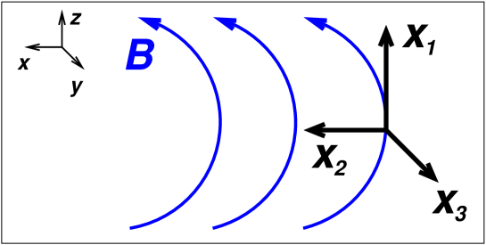
Figure 2: Sketch of curvilinear coordinates for curvilinear or dipole magnetic field configurations.

Let coordinates ($x_{1}$, $x_{2}$, $x_{3}$), such that the coordinate $x_{1}$ is directed along field lines, the coordinate $x_{2}$ is in the direction of the radius of curvature, and the coordinate $x_{3}$ is in the azimuthal direction, see Fig. 2 . The equation of motion can be written in components as

$$\rho\partial_{tt}\xi_{1} = 0,$$ (17)

$$\rho\partial_{tt}\xi_{2} = \frac{B}{h_{1}h_{2}}\left[\partial_{2}(\partial_{2}Bh_{3}\xi_{2}+\partial_{3}Bh_{2}\xi_{3})+\partial_{1}\left(\frac{h_{2}}{h_{1}h_{3}}\partial_{1}Bh_{3}\xi_{2}\right)\right],$$ (17)

$$\rho\partial_{tt}\xi_{3} = \frac{B}{h_{1}h_{3}}\left[\partial_{3}(\partial_{2}Bh_{3}\xi_{2}+\partial_{3}Bh_{2}\xi_{3})+\partial_{1}\left(\frac{h_{3}}{h_{1}h_{2}}\partial_{1}Bh_{2}\xi_{3}\right)\right],$$ (17)

where $h_{1}$, $h_{2}$, $h_{3}$ are the metric (Lamé) coefficients. We limited ourselves to a 2-dimensional problem in the $x_{1}x_{2}$ (or $xz$) plane. Here $\partial_{t}=\partial/\partial t$ and $\partial_{i}=\partial/\partial x_{i}$.

In a strong magnetic field the usual definition of the Alfvén velocity, $v_{\rm A}^{2}=B^{2}/4\pi\rho$, is failed by resulting values larger than speed of light, $c$. To avoid of such confusion we define the relativistic Alfvén velocity by using enthalpy

$$h=\frac{c^{2}\rho+B^{2}/4\pi}{c^{2}}$$ (18)

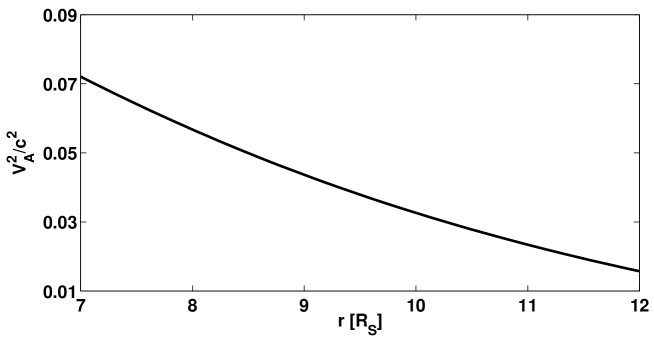
Figure 3: $v_{\rm A}^{2}$ in equatorial plane

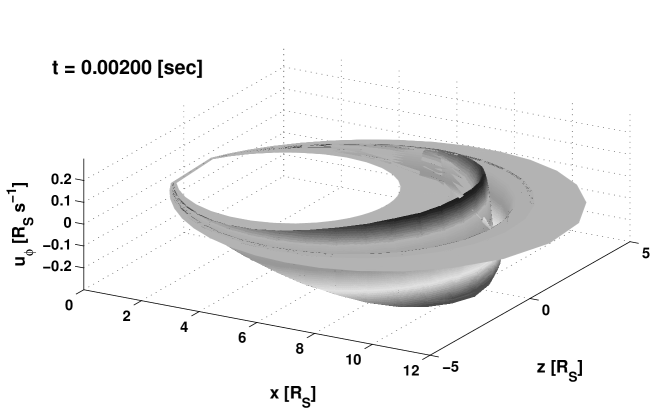
Figure 4: Azimuthal velocity, $v_{\phi}$, profile for a FLR in a dipole, neutron star’s magnetosphere. $R_{s}$ is in units of the star radius.

rather than the plasma density $\rho$. So the Alfvén velocity shall be $v_{\rm A}^{2}=B^{2}/4\pi h$ (Fig. 3). As shown in Fig. 3 close to the star the relativistic Alfvén velocity saturates at the speed of light, ie. $v_{\rm A}\sim c$. Such definition for the Alfvén velocity is extensively used in studying of the relativistic jets dynamics in quasars. Figure 4 shows a computational model of the profile of the azimuthal component of the velocity. In a FLR with small azimuthal wavenumber, the displacement and velocity fields are predominantly azimuthal, with a $180^{o}$ phase shift across the position of the resonance.

4 Magnetohydrodynamics in the presence of ambient flow

As discussed above, FLRs have been used to model auroral observations in the Earth’s magnetosphere. Although the occurrence of these resonances is generic and likely to be excited in any magnetosphere with input of compressional of energy, one must carefully evaluate the differences between the Earth and neutron star magnetospheres. In the case of the Earth’s magnetosphere, due to the small gravitational attraction of the Earth and also its large distance from the Sun, the solar wind more or less hits the whole Sunward side of the geomagnetosphere, and produces the so-called bow shock structure at the outer boundary. However, the strong gravity of the neutron star creates a supersonic converging flow long before the flow hits the star’s magnetosphere. Such a localized flow is able to change the structure of the magnetosphere in local areas particularly in the equatorial plane. In addition, the highly variable nature of the exterior flow can change the magnetosphere’s structure with time dramatically. The large flux of plasma stresses the outer star’s magnetosphere and creates a relatively high plasma density throughout the magnetic field. The plasma then flows along the field lines, an interior flow, until it hits the star’s surface near the magnetic poles, see Fig. 1. Furthermore, the strong magnetic field of the star, the rapid rotation, and the intense radiation pressure from the surface must be added to the problem.

One of the most prominent differences between magnetospheres of accreting neutron stars and the Earth’s magnetosphere is the presence of an ambient flow along the field lines where the resonance takes place (Ghosh & Lamb, 1991). In this section we study the excitation of FLRs by considering such plasma flow in the magnetosphere.

The presence of a flow ${\bf v}$ in the plasma adds more modes to the plasma waves. In general, such flow is a combination of plasma flow along the magnetic field lines, ${\bf v}_{p}$, and rotational motion of the plasma around the star with angular velocity $\Omega$, ie. ${\bf v}={\bf v}_{p}+\mbox{\boldmath$\Omega$}\times{\bf r}$, see Eq. (2). The existence of ${\bf v}_{p}$ itself allows a non-zero parallel component (relative to the magnetic field) of displacement that vanishes in a cold plasma with ${\bf v}_{p}=0$. We note that this component is responsible for modulating the infalling plasma flow toward the star surface with FLRs’ frequencies and producing the observed X-ray fluxes, see Eq. (22a) below. We will back to this point later.

As we mentioned earlier, due to the relatively strong magnetic field in accreting neutron stars one needs to consider the relativistic Alfvén velocity as

$$v_{\rm A}^{2}=\frac{c^{2}}{c^{2}\rho+B^{2}/4\pi}~{}\frac{B^{2}}{4\pi}\,.$$ (19)

See Eq. (18) for the definition of the enthalpy. Since the plasma pressure in neutron stars is negligible compared to magnetic pressure (Ghosh et al., 1977) we are using a cold plasma approximation in this section. Again we use a linear approximation to obtain a dispersion relation with resonant coupling. Since the gravity acts in a direction nearly perpendicular to field line for most of the infall of the matter, we can assume that the flow is nearly constant. This simplifies the derivation significantly.

The linearized magnetohydrodynamic equations in the presence of an ambient flux can be obtained from Eqs. (9a) as

$$h\left({\partial\delta{\bf v}\over\partial t}+{\partial{\bf v}\over\partial t}+{\bf v}\cdot\mbox{\boldmath$\nabla$}\delta{\bf v}+\delta{\bf v}\cdot\mbox{\boldmath$\nabla$}{\bf v}\right)=-\mbox{\boldmath$\nabla$}\delta p+{\mbox{\boldmath$\nabla$}p\over h}\delta h$$

$$\hskip 142.26378pt+{1\over 4\pi}\delta{\bf B}\times\mbox{\boldmath$\nabla$}\times{\bf B}+{1\over 4\pi}{\bf B}\times\nabla\times\delta{\bf B},$$ (20a)

$${\partial\delta{\bf B}\over\partial t}=\mbox{\boldmath$\nabla$}\times(\delta{\bf v}\times{\bf B}+{\bf v}\times\delta{\bf B}),$$ (20b)

$$({\partial\over\partial t}+{\bf v}\cdot\mbox{\boldmath$\nabla$})\delta p+\delta{\bf v}\cdot\mbox{\boldmath$\nabla$}p=-\gamma(\delta p\mbox{\boldmath$\nabla$}\cdot{\bf v}+p\mbox{\boldmath$\nabla$}\cdot\delta{\bf v}),$$ (20c)

where $\delta{\bf v}=\partial{\mbox{\boldmath$\xi$}}/\partial t$. The time scale of the ambient flow variations is much longer than time scale of the excited MHD perturbations, so $\partial{\bf v}/\partial t=0$. Furthermore, we consider the slow rotation approximation and so neglect the toroidal field ${\bf B}_{\phi}$, Eq. (2), to avoid complexities. Such assumptions may not meet the actual configuration precisely. Nevertheless, these assumptions simplify our calculations significantly.

Separating Eqs. (4) into parallel and perpendicular components relative to the ambient magnetic field and assuming perturbed quantities in the form of

$$\delta({\bf r},t)=\delta({\bf r}_{\perp})e^{-i(\omega t-k_{||}x_{||})}\,,$$ (21)

we find

$$(-i\omega+ik_{||}v_{||})\xi_{||}=-\frac{k_{||}v^{2}_{\rm s}}{\omega-k_{||}v_{||}}\mbox{\boldmath$\nabla$}\cdot{\mbox{\boldmath$\xi$}}-({\mbox{\boldmath$\xi$}}_{\perp}\cdot\mbox{\boldmath$\nabla$}_{\perp})v_{||}\,,$$ (22a)

$$((\omega-k_{||}v_{||})^{2}-k_{||}^{2}v_{\rm A}^{2}){\mbox{\boldmath$\xi$}}_{\perp}=\frac{\omega-k_{||}v_{||}}{\omega}\frac{\mbox{\boldmath$\nabla$}_{\perp}\delta P}{h}-\frac{\omega-k_{||}v_{||}}{\omega}\frac{\mbox{\boldmath$\nabla$}_{\perp}p}{h^{2}}\delta h\,,$$ (22b)

$$(-i\omega+ik_{||}v_{||})\delta B_{||}=i\omega B(\mbox{\boldmath$\nabla$}_{\perp}\cdot{\mbox{\boldmath$\xi$}}_{\perp})+i\omega({\mbox{\boldmath$\xi$}}_{\perp}\cdot\mbox{\boldmath$\nabla$}_{\perp})B+(\delta{\bf B}_{\perp}\cdot\mbox{\boldmath$\nabla$}_{\perp})v_{||}\,,$$ (22c)

$$(-i\omega+ik_{||}v_{||})\delta{\bf B}_{\perp}=\omega k_{||}B{\mbox{\boldmath$\xi$}}_{\perp}\,,$$ (22d)

$$(-i\omega+ik_{||}v_{||})\delta p=i\omega({\mbox{\boldmath$\xi$}}_{\perp}\cdot\mbox{\boldmath$\nabla$}_{\perp})p+\gamma(-\omega k_{||}p\xi_{||}+i\omega p\mbox{\boldmath$\nabla$}_{\perp}\cdot{\mbox{\boldmath$\xi$}}_{\perp})\,,$$ (22e)

$$-\frac{\delta P}{h}=\frac{\omega}{\omega-k_{||}v_{||}}(v_{\rm s}^{2}+v_{\rm A}^{2})\mbox{\boldmath$\nabla$}\cdot{\mbox{\boldmath$\xi$}}-\frac{i\omega k_{||}v_{\rm A}^{2}}{\omega-k_{||}v_{||}}\xi_{||}+\frac{\omega k_{||}v_{\rm A}^{2}}{(\omega-k_{||}v_{||})^{2}}({\mbox{\boldmath$\xi$}}_{\perp}\cdot\mbox{\boldmath$\nabla$}_{\perp})v_{||}\,,$$ (22f)

where $\omega$ is the eigenfrequency, $k_{||}$ is the wave number in the parallel direction, ${\bf v}_{p}=v_{||}{\bf B}/B$, $v_{\rm s}=\sqrt{\gamma p/h}$ is the sound velocity, and $P=p+B^{2}/8\pi$ is the total plasma pressure (fluid $+$ field). Note that we assumed that all ambient quantities are function of ${\bf r}_{\perp}$ only. Equation (22a) shows that the plasma displacement parallel to the ambient field does not vanish even in the cold plasma approximation ($p=0$). The non-zero $\xi_{||}$ can affect and then modulate the motion of plasma along the field lines. Such modulation will occur at frequency of the resonant shear Alfvén waves $\omega$ as seen in the observed X-ray fluxes.

To analyze the problem analytically, we consider here again the rectilinear magnetic field configuration. We note that although this configuration may not be suitable for the accreting neutron star, it provides us a descriptive picture that can be applicable to QPOs. Setting the magnetic field in z-direction with gradients in the ambient parameters in the x-direction, $v_{||}({\bf r}_{\perp})=v_{p}(x)$, and

$$\delta({\bf r},t)=\delta(x)e^{-i(\omega t-k_{y}y-k_{z}z)},$$ (23)

Eqs. (22a) in the cold plasma approximation ($p=0$) can be combined into one differential equation in the form of Eq. (11)

$$\frac{d^{2}\xi_{x}}{dx^{2}}+\frac{\Xi^{\prime}(x)}{\Xi(x)}\frac{d\xi_{x}}{dx}+\frac{(\omega-k_{z}v_{p})^{2}-(k_{y}^{2}+k_{z}^{2})v_{\rm A}^{2}}{v_{\rm A}^{2}}\xi_{x}=0,$$ (24)

where

$$\Xi(x)=\frac{v_{\rm A}^{2}}{\omega-k_{z}v_{p}}~{}\frac{(\omega-k_{z}v_{p})^{2}-k_{z}^{2}v_{\rm A}^{2}}{(\omega-k_{z}v_{p})^{2}-(k_{y}^{2}+k_{z}^{2})v_{\rm A}^{2}}\,.$$ (25)

Note that here $v_{p}=v_{p}(x)$ and $v_{\rm A}=v_{\rm A}(x)$ are function of $x$. For $v_{p}=0$ Eq. (25) reduces to one obtained in section 3.3, Eq. (13), as expected. The condition $\Xi(x)=0$ yields the following modes:

$$\omega^{\pm}=k_{z}(v_{p}\pm v_{\rm A}).$$ (26)

The resulting modes are combination of a compressional mode $k_{z}v_{p}$ due to the plasma flow and a shear Alfvén mode $k_{z}v_{\rm A}$. They produced two frequency peaks in the spectrum that vary with time if the velocities change with time. The value of $k_{z}\sim\pi/L$ where $L$ is the length of field line and is in order of radius of neutron star, $L\sim R_{s}$. Therefore, for $R_{s}\sim 10^{6}$ cm and $v_{\rm A}\sim v_{p}\sim 3\times 10^{8}$ cm s^-1 we get $\omega^{+}\sim 1000$ Hz that is comparable with frequencies of the observed quasi-periodic oscillations. In the limit $v_{p}\ll v_{\rm A}$ these modes become a single mode of a regular Alfvén resonance. In the case of $v_{\rm A}\ll c$ these modes become consistent with a single mode (17). For a superalfvénic flow, ie. $v_{\rm A}\ll v_{p}$, however, the MHD Alfvén waves and the resulting FLRs are suppressed due to propagation of the hydrodynamical wave, $k_{z}v_{p}$. Therefore, no FLRs are likely to occur at this level. This can be understood from Eq. (25) that for superalfvénic plasma flow reduces to

$$\Xi(x)\simeq\frac{v_{\rm A}^{2}}{\omega-k_{z}v_{p}}\frac{k_{z}^{2}}{k_{y}^{2}+k_{z}^{2}}\,,$$ (27)

where as $\omega\rightarrow k_{z}v_{p}$, $\Xi(x)\rightarrow\infty$. As a result, we expect that the FLR occurs where $v_{p}$ and $v_{\rm A}$ are comparable. Using the flow velocity and the shear Alfén velocity definitions (see below), one might expect that the FLRs likely occur at $R_{s}<r<100R_{s}$.

Approximating the plasma inflow velocity with the free fall velocity $v_{p}\sim v_{\rm ff}(r)$ and $v_{\rm A}\sim B(r)/\sqrt{4\pi\rho_{\rm ff}}$ where $\rho_{\rm ff}=\dot{M}/(v_{\rm ff}~{}4\pi r^{2})$ is the free fall mass density, one can rewrite Eq. (26) as:

$$\omega^{\pm}(r) \simeq k_{z}\left(\frac{}{}(2GM/r)^{1/2}\pm(B(r)^{2}/4\pi\rho_{\rm ff}(r)~{})^{1/2}\frac{}{}\right),$$ (28)

$$\simeq k_{z}(v_{p}(R_{s})x^{-1/2}\pm v_{\rm A}(R_{s})x^{-9/4})\,,$$

where $v_{p}(R_{s})=(2GM/R_{s})=1.6\times 10^{10}(M/M_{\odot})^{1/2}(R_{s}/10\,{\rm km})^{-1/2}$ cm s^-1 and $v_{\rm A}(R_{s})=B/\sqrt{4\pi\rho_{\rm ff}(R_{s})}\simeq 3\times 10^{10}\mu_{26}\dot{M}_{17}^{-1/2}(M/M_{\odot})^{1/4}(R_{s}/10\,{\rm km})^{-9/4}$ cm s^-1 are inflow and Alfvén velocities at the surface of the star. Here $\mu_{26}$ is the magnetic field dipole moment at the surface of star in units of $10^{27}$ G cm^-3, $\dot{M}_{17}$ is the mass of accretion rate in units of $10^{17}$ g s^-1, $x=r/R_{s}$, and $R_{s}$ is the radius of star. Figures 5 and 6 show the variation of purely Alfvén resonance frequencies ($v_{p}=0$) or FLRs, as a function of distance from the star and magnitude of Alfvén velocity. It is clear that the closer to the star and/or the larger the Alfvén velocity the higher the frequency. Therefore, for an Alfvén velocity say $v_{\rm A}\sim.1c$ one can get a frequency about $1000$ Hz at $r\simeq 2R_{s}$ as we expected. Furthermore, since the Alfvén velocity depends on the enthalpy (or density) of the plasma which varies from time to time due to several processes such as magneto-turbulence at boundaries during the accretion, the resulting FLRs frequencies will also vary with time. In addition, the position that the resonance takes place, is also subject to change in time due to the time varying accretion rate. Such time varying behavior causes time varying frequencies or quasi-periodic frequencies as observed.

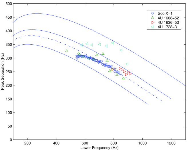
Figure 7: Variation of peak separation frequency $\Delta\nu$ with the upper frequency $\nu_{2}$. The resulting curves are compared with the observed values for different system. The solid curves from bottom to top correspond to $\nu_{2}\sim 1170,\,1350,$ and $1548$ Hz at $r=R_{s}$. The dashed curve corresponds to $\nu_{2}=1278$ Hz at $r=R_{s}$.

Setting $\omega^{-}$ as the observed peak separation frequency $\Delta\nu\sim\omega^{-}$, and $\omega^{+}$ as the upper QPO frequency $\nu_{2}\sim\omega^{+}$, we can compare our results with observations. Figures 7 and 8 show the variation of $\Delta\nu$ vs $\nu_{1}$ and $\nu_{2}$, respectively, along with the observed values. The curves are drawn by assuming the ratio $v_{\rm A}/v_{p}\simeq.8$ ar $r=R_{s}$ where from bottom to top correspond to upper frequency $\nu_{2}\sim 1170$ Hz, $1350$ Hz, and $1548$ Hz at $r=R_{s}$, respectively. As shown by observations, the value of $\Delta\nu$ decreases whenever the magnitude of $\nu_{2}$ decreases (sufficiently) and/or it increases. Such behavior is expected in our model (see Fig. 8).

Furthermore, the lower QPO frequency can be obtained from $\nu_{1}=\nu_{2}-\Delta\nu\sim 2k_{z}v_{\rm A}$. As a result, $\nu_{1}$ to $\nu_{2}$ we obtain the frequency ratio

$$\nu_{1}/\nu_{2}=2v_{\rm A}/(v_{p}+v_{\rm A})=2/(1+v_{p}/v_{\rm A})\,.$$ (30)

It is clear that depending on the relation between the plasma flow velocity $v_{p}$ and the Alfvén velocity $v_{\rm A}$, one can obtain different frequency ratios. For example, if the velocity inflow plasma is $2$ ($7/3\sim 2.3$) times bigger than the Alfvén velocity, ie. $v_{p}=2v_{\rm A}$, one can get $2:3$ ($3:5$) ratio. For a free falling plasma along the lines of a dipolar magnetic field, $v_{p}^{2}(r)\propto r^{-1}$, whereas $B^{2}(r)/4\pi\rho(r)\propto r^{-9/2}$, the condition $v_{p}\sim 2v_{\rm A}$ ($v_{p}\sim 2.3v_{\rm A}$) is satisfied at $r\sim 3R_{s}\sim 1.5r_{\rm A}$. The occurrence of FLRs is very likely at this distance from the star.

Such pairs of high frequencies with $2:3$ frequencies ratio have been observed in the X-ray flux of almost all neutron stars in LMXBs and black hole systems (the $3:5$ ratio has seen in one source), and it would appear this feature is common to those systems. However, the existence of such rational ratios is still a mystery. In black hole systems, it has been suggested that such frequencies correspond to a trapped g-mode or c-mode of disk oscillation in the Kerr metric, see for example Kato (2001) and references therein. In neutron star systems they are explained as the fundamental and the first harmonic of the non-axisymmetric ($m=1$) g-mode (Kato, 2002, 2003). Further, Rezzolla et al. (2003a, b) studied small perturbations of an accretion torus orbiting close to the black hole and modelled the observed high QPO frequencies with basic p-modes of relativistic tori. They showed that these modes behave as sound waves trapped in the torus with eigenfrequencies appearing in sequence 2:3:4:… Abramowicz et al. (2003) also proposed that the observed rational ratios of frequencies may be due to the strong gravity of the compact object and a non-linear resonance between radial and vertical oscillations in accretion disks.

5 Discussion

In the present work, we have studied the interaction of an accretion disk with a neutron star magnetosphere in the LMXBs. The recent extensive observations reveal the existence of quasi-periodic oscillations in the X-ray fluxes of such stars. These oscillations, with frequencies range from $10$ Hz to $1200$ Hz, have been the subject of several theoretical and observational investigations. Based on theoretical models for the observed aurora in the earth magnetosphere, we have introduced a generic magnetospheric model for accretion disk-neutron star systems to address the occurrence and the behavior of the observed QPOs in those systems. In order to explain those QPOs consistently, we consider the interaction of the accreting plasma with the neutron star’ magnetosphere. Due to the strong gravity of the star, a very steep and supersonic flow hits the magnetosphere boundary and deforms its structure drastically. Such a plasma flow can readily excite different MHD waves in the magnetosphere, such as the shear Alfvén waves.

In the Earth’s magnetosphere, occurrence of aurora is a result of resonant coupling between the shear Alfvén waves and compressional waves (produced by the solar wind). These resonances are known as FLRs that are reviewed in detail in section 3 of this paper. We argue that such resonant coupling is likely to occur in neutron star magnetospheres during its interaction with accreting plasma. We formulated an improved FLR by considering a plasma flow moving with velocity $v_{p}$ along the magnetic field lines. Such flow is likely to occur in neutron star magnetosphere (Ghosh et al., 1977). For a simple geometry, the rectilinear magnetic field, and in the presence of a plasma flow we found: (a) two resonant hydrodynamical-MHD modes with frequencies $\omega^{\pm}=k_{z}(v_{p}\pm v_{\rm A})$. (b) the resulting frequencies for $k_{z}\sim\pi/R_{s}\sim 3\times 10^{-6}$ cm^-1 and typical flow and/or Alfvén velocity $\sim.1c$ will be in kHz range. Our results match the kHz oscillations observed in the X-ray fluxes in LMXBs. As shown in figures 5 and 6, the closer to the star and/or the larger the Alfvén velocity the higher the frequency. (c) the quasi-periodicity of the observed oscillations can be understood by noting that due to several processes such as magneto-turbulence at boundaries and the time varying accretion rate, the FLR frequencies may vary with time. (d) a non-zero plasma displacement along the magnetic field lines $\xi_{||}$. Such a displacement that oscillates with resulting frequencies $\omega^{\pm}$ modulates the flow of the plasma toward the surface of neutron star. As a result, the X-ray flux from the star will show these frequencies as well. (e) setting $\Delta\nu=\omega^{-}$ and $\nu_{2}=\omega^{+}$, one can well explain the behavior of the peak separation frequency $\Delta\nu$ relative to the upper QPO frequency $\nu_{2}$. As observed, the value of $\Delta\nu$ decreases as the magnitude of $\nu_{2}$ decreases and/or increases. Figure 8 clearly shows such behavior. (f) for $v_{p}\sim 2v_{\rm A}$ at $r\sim 3R_{s}$, the frequency ratio $\nu_{1}/\nu_{2}$ is comparable with the observed frequency ratio $2:3$.

Interestingly, using the observed values of QPO frequencies, one can determine the average mass density and the magnetic field density of the star as

$$k_{z}v_{p}(r)=(1/2)(\nu_{2}+\Delta\nu)=(\nu_{2}-\nu_{1}/2),$$ (31a)

$$k_{z}v_{\rm A}(r)=(1/2)(\nu_{2}-\Delta\nu)=\nu_{1}/2\,.$$ (31b)

Therefore,

$$M_{s}/R_{s}^{3}\simeq(1/8\pi^{2}G)x^{3}(\nu_{2}+\Delta\nu)^{2},$$ (32a)

$$\mu_{s}\simeq(32\pi^{4}G)^{-1/4}R_{s}^{5/2}\dot{M}^{1/2}(M_{s}/R_{s}^{3})^{-1/4}x^{13/4}\nu_{1},$$ (32b)

where $k_{z}\simeq\pi/r$, $\mu_{s}=B_{0}R_{s}^{3}$,$x=r/R_{s}$, and $B_{0}$ is the magnetic field strength at the surface of the star. In table 1, we calculate the average density $M_{s}/R_{s}^{3}$ and magnetic dipole moment $\mu_{s}$ of the star for a fixed value $x=10$. Note that larger frequencies may occur at smaller distances, ie. $x<10$. Our results are comparable with realistic neutron star parameters.

Furthermore, our model is able to explain those low frequency ($\sim 10$ Hz) quasi-periodic oscillations observed in the rapid burster such as MXB 1730-335 and GRO J1744-28 (Masetti et al., 2000). Such low frequencies can be extracted from the model by considering smaller inflow/Alfvén velocity and/or further distances from the star.

Nevertheless, in order to avoid a number of complexities in our calculations, we used approximations such as slow rotation and cold plasma. These assumptions may put some restriction on the validity of our model and results. Future studies will be devoted to overcoming those restrictions.

VR wishes to thank Mariano Mendez for kindly providing QPO data. This research was supported by the National Sciences and Engineering Research Council of Canada.

—————————————————————————————-

Table 1: Observed frequencies of kilohertz QPOs in Z and atoll sources

		$\nu_{1}$	$\nu_{2}$	$\Delta\nu$	$M_{s}/R_{s}^{3}$	$\mu_{s}$
Source	Type	(Hz)	(Hz)	(Hz)	($10^{14}$ g cm-3)	($10^{26}$ G cm3)
Sco X$-$1	Z	565	870	307$\pm$5	2.6	3.8
GX 5$-$1	Z	660	890	298$\pm$11	2.7	4.1
GX 17+2	Z	780	1080	294$\pm$8	3.5	4.8
Cyg X$-$2	Z	660	1005	346$\pm$29	3.4	4.1
GX 340+0	Z	565	840	339$\pm$8	2.6	3.8
GX 349+2	Z	710	980	266$\pm$13	2.9	4.5
4U 0614+09	atoll	825	1160	312$\pm$2	4.1	4.8
4U 1608$-$52	atoll	865	1090	225$\pm$12	3.2	1.7
4U 1636$-$53	atoll	950	1190	251$\pm$4	3.9	5.4
4U 1702$-$43	atoll	770	1085	315$\pm$11	3.7	4.8
4U 1705$-$44	atoll	775	1075	298$\pm$11	3.5	4.8
4U 1728$-$3	atoll	875	1160	349$\pm$2	4.3	5.1
KS 1731$-$260	atoll	900	1160	260$\pm$10	3.8	5.4
4U 1735$-$44	atoll	900	1150	249$\pm$15	3.7	5.4
4U 1820$-$30	atoll	795	1075	278$\pm$11	3.4	4.8
Aql X$-$1	atoll	930	1040	241$\pm$9	3.1	5.7
4U 1915$-$05	atoll	655	1005	348$\pm$11	3.4	4.1
XTE J2123$-$058	atoll	845	1100	255$\pm$14	3.4	5.1

Low ($\nu_{1}$) and high ($\nu_{2}$) QPO frequencies with corresponding peak separation ($\Delta\nu$) observed in Z and atoll sources. Only one series data is given as example, for further detail see van der Klis (2000). Values of $M_{s}/R_{s}^{3}$ and $\mu_{s}$ are calculated from Eq. (32a) for a fixed value $x=10$. We note that larger frequencies may be occurred at smaller distances, $x<10$.

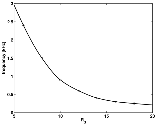
Figure 5: Radial profile of the frequency of a FLR. The closer to the star the higher the frequency. Here $v_{\rm A}=.5c$.

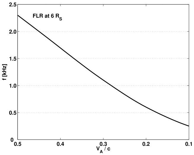
Figure 6: Frequency of a FLR at $6R_{s}$ from the star as function of Alfvén wave velocity. The larger the Alfvén velocity the higher the frequency.

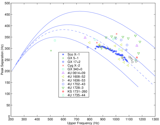
Figure 8: Variation of peak separation frequency $\Delta\nu$ with the upper frequency $\nu_{2}$. The resulting curves are compared with the observed values for different system. The solid curves from bottom to top correspond to $\nu_{2}\sim 1170,\,1350,$ and $1548$ Hz at $r=R_{s}$. The dashed curve corresponds to $\nu_{2}=1278$ Hz at $r=R_{s}$.

References

- Abramowicz et al. (2003) Abramowicz M. A., et al., 2003, PASJ , 55, 467
- Alpar & Shaham (1985) Alpar M. A. , & Shaham J., 1985, Nature , 316, 239
- Bildsten & Strohmayer (2003) Bildsten L., & Strohmayer T., 2003, To appear in Compact Stellar X-Ray Sources, eds. W.H.G. Lewin & M. van der Klis, Cambridge University Press, pre-print: astro-ph/0301544
- Budden (1985) Budden K. G., 1985, The propagation of radio waves, Cambridge Univ. Press
- Chen & Hasegawa (1974) Chen L., & Hasegawa A., 1974, J. Geophys. Res., 79, 1024
- Dobias (2002) Dobias P., 2002, PhD thesis, University of Alberta
- Dobias et al. (2004) Dobias P., Samson J. C., & Voronkov I. O., 2004, Phys. Plasmas, in press
- Einstein (1915) Einstein A., 1915, Preuss. Akad. Wiss. Berlin, Sitzber., 47, 831
- Elsner & Lamb (1977) Elsner R. F., & Lamb F. K., 1977, ApJ , 215, 897
- Elsner & Lamb (1984) Elsner R. F., & Lamb F. K., 1984, ApJ , 278, 326
- Ghosh & Lamb (1991) Ghosh P., & Lamb F. K., 1991, Neutron Stars: Theory and Observation, J. Ventura & D. Pines (eds.), 363, Kluwer Academic Publisher
- Ghosh et al. (1977) Ghosh P., Lamb F. K., & Pethick C. J., 1977, ApJ , 217, 578
- Giacconi et al. (1971) Giacconi R. et al., 1971, ApJL, 167, 67
- Harrold & Samson (1992) Harrold B. G. & Samson J. C., 1992, Geoph. Res. Let., 19, 1811
- Hasegawa (1976) Hasegawa A., 1976, J. Geophys. Res., 81, 5083
- Hasinger et al. (1986) Hasinger M. et al., 1986, Nature, 319, 469
- Kato (2001) Kato S., 2001, PASJ, 53, 1
- Kato (2002) Kato S., 2001, PASJ, 54, 39
- Kato (2003) Kato S., 2003, PASJ, 55, 801
- Lamb & Miller (2001) Lamb F. K., & Miller M. C., 2001, ApJ , 554, 1210
- Lamb et al. (1985) Lamb F. K., Shibazaki N., Alpar M. A., & Shaham J., 1985, Nature , 317, 681
- Landau & Lifshitz (1992) Landau L. D., & Lifshitz E. M., 1992, Elektrodinamika Splosnych Sred, Nauka, Moscow
- Liu (1997) Liu W. W., 1997, J. Geophys. Res., 102, 4927
- Marković & Lamb (1998) Marković D., & Lamb F. K., 1998, ApJ , 507, 316
- Masetti et al. (2000) Masetti N., et al., 2000, A&A , 363, 188
- Middleditch & Priedhorsky (1986) Middleditch, J., & Priedhorsky, W. C., 1986, ApJ, 306, 230
- Mestel (1961) Mestel L., 1961, MNRAS , 122, 473
- Mestel (1968) Mestel L., 1968, MNRAS , 138, 359
- Miller et al. (1996) Miller M. C., Lamb F. K., & Psaltis D., 1996, American Astronomical Society, 189th AAS Meeting, # 44.11; Bulletin of the American Astronomical Society, Vol. 28, p.1329, pre-print: astro-ph/9609157v1
- Miller et al. (1998) Miller M. C., Lamb F. K., & Psaltis D., 1998, ApJ 508, 791
- Morsink & Stella (1999) Morsink S. M., & Stella L., 1999, ApJ , 513, 827
- Ohtani & Tamao (1993) Ohtani S. I., & Tamao T., 1993, J. Geophys. Res., 98, 19369
- Rezania & Karmand (2003) Rezania V., & Karmand S., 2003, A&A , 410, 967
- Rezzolla et al. (2003a) Rezzolla L., et al., 2003a, MNRAS , 344, L37
- Rezzolla et al. (2003b) Rezzolla L., Yoshida S., & Zanotti O., 2003b, MNRAS , 344, 978
- Rickard & Wright (1994) Rickard G. J., & Wright A. N., 1994, J. Geophys. Res., 99, 13455
- Samson (1991) Samson J. C., 1991, in Geomagnetism, Vol. 4, J. A. Jacobs ed., 482, Academic press
- Samson & Rankin (1994) Samson J. C., & Rankin R., 1994, in Solar Wind Sources of Magnetospheric Ultra-Low-Frequency Waves, Geophys. Monograph Ser., Vol. 81, edited by M. J. Engberston, K. Takahashi, & M. Scholder, p. 253, AGU, Washington, D. C.
- Samson et al. (1996) Samson J. C., Cogger L. L., & Pao Q., 1996, J. Geophys. Res., 101, 17373
- Samson et al. (2003) Samson J. C., Rankin R., & Tikhonchuk V. T., 2003, Annales Geophysicae, 21, 933
- Schreier et al. (1972) Schreier E. J. et al., 1972, ApJL, 172, 79
- Southwood (1974) Southwood D. J., 1974, Space Sci. Rev., 22, 483
- Stella & Vietri (1998) Stella L., & Vietri M., 1998, ApJ , 492, L59
- Stella & Vietri (1999) Stella L., & Vietri M., 1999, Phys. Rev. Lett. , 82, 17
- Stella et al. (1999) Stella L., Vietri M., & Morsink S. M., 1999, ApJ , 524, L63
- Stix (1992) Stix T. H., 1992, Waves in Plasma, AIP
- Tananbaum et al. (1972) Tananbaum H. et al., 19872, ApJL, 174, 143
- Taylor & Walker (1984) Taylor J. P. H., & Walker A. D. M., 1984, Plant. Space Sci., 32, 1119
- Thirring & Lense (1918) Thirring H., & Lense J., 1918, Phys. Z., 19, 156
- van der Klis et al. (1985) Van der Kils, M. et al., 1985, Nature, 316, 225
- van der Klis (2000) Van der Kils, M., 2000, Annual Review of Astronomy and Astrophysics, 38, 717
- Zhang (2004) Zhang, C., 2004, pre-print astro-ph/0402028