The HCO⁺ Emission Excess in Bipolar Outflows

Abstract

A plausible model is proposed for the enhancement of the abundance of molecular species in bipolar outflow sources. In this model, levels of HCO⁺ enhancement are considered based on previous chemical calculations, that are assumed to result from shock-induced desorption and photoprocessing of dust grain ice mantles in the boundary layer between the outflow jet and the surrounding envelope. A radiative transfer simulation that incorporates chemical variations within the flow shows that the proposed abundance enhancements in the boundary layer are capable of reproducing the observed characteristics of the outflow seen in HCO⁺ emission in the star forming core L1527. The radiative transfer simulation also shows that the emission lines from the enhanced molecular species that trace the boundary layer of the outflow exhibit complex line profiles indicating that detailed spatial maps of the line profiles are essential in any attempt to identify the kinematics of potential infall/outflow sources. This study is one of the first applications of a full three dimensional radiative transfer code which incorporates chemical variations within the source.

1 Introduction

The complex morphologies of molecular outflows have been identified in numerous studies, mostly based on high resolution, interferometric CO and optical surveys (eg. Arce & Goodman, 2001, 2002; Lee et al. 2000, 2002). These surveys show that the molecular distributions are generally composed of a large scale, poorly collimated low velocity outflow that essentially traces the interaction between a surrounding molecular cloud envelope and a collimated high velocity jet. These morphologies are hard to interpret unambiguously but often resemble limb-brightened shells or sheaths surrounding cavities.

Observations at single-dish resolution suggest that the abundance of HCO⁺ in star forming cores with bipolar outflows may be enhanced by a factor of up to 100–1000$\times$ relative to dark-cloud values - for example, a fractional abundance of $4\times 10^{-8}$ is implied in the case of the Class 0 source B335 (Rawlings, Taylor and Williams 2000). This, and similar observations, provided the basis for the models of Rawlings et al. (2000) in which the enhancement of HCO⁺ originates in the turbulent mixing layer which is the interface between the high velocity outflow and the quiescent or infalling core gas which it is steadily eroding. The molecular enrichment is driven by the desorption of molecular-rich ice mantles, followed by photochemical processing by shock-generated radiation fields. Thus, CO and H₂O are released following mantle evaporation. The CO is then photodissociated and the C that is produced is photoionized by the shock-induced radiation field that is generated in the interface:

$${\rm CO}+{\rm h}\nu\longrightarrow{\rm C}+{\rm O}$$

$${\rm C}+{\rm h}\nu\longrightarrow{\rm C}^{+}+{\rm e}^{-}$$

The subsequent reactions of C⁺ with H₂O lead to an enhancement of the HCO⁺ abundance:

$${\rm C}^{+}+{\rm H}_{2}{\rm O}\longrightarrow{\rm HCO}^{+}+{\rm H}$$

This abundance enhancement is only temporary, and progresses as a wave that fans out from the interface into the core. Such behaviour is both qualitatively and quantitatively consistent with the scenario proposed by Velusamy and Langer (1998) for B5 IRS1 on the basis of their ¹²CO (2-1) and C¹⁸O (2-1) observations; the data clearly show a parabolic outflow cavity that appears to be steadily widening, so that the opening angle is growing at a rate of 0.006^∘yr^-1. An extension of the chemistry to a larger species/reaction set by Viti, Natarajan and Williams (2002) confirmed this result and concluded that other molecular tracers, such as H₂CS, SO, SO₂ and CH₃OH could be similarly affected.

At higher resolutions, aperture synthesis observations are capable of identifying the morphology of the interaction between the jets and their surroundings. Hogerheijde et al. (1998) made high resolution HCO⁺ J=1$\to$0 observations using the Owens Valley Millimetre Array (OVRO) towards a number of low mass YSOs. One of the most interesting results from that survey was the detection of compact emission associated with the walls of an outflow cavity in L1527 (Hogerheijde et al. 1998, figure 1). The ${}^{12}{\rm CO}3-2$ outflow lobes are well-developed, with lengths of $\sim 0.12~{}\rm pc$ and a large opening angle ($\sim 90^{\circ}$). The single dish observations of Hogerheijde et al (1997) show that the HCO⁺ emission is confined to a smaller scale, $\sim 0.015$ to 0.022 pc, in the center of the flow. The interferometric observations with higher angular resolution show that much of this HCO⁺ emission originates in the boundary of the lobes of the CO outflow rather than in the quiescent core of the cloud surrounding the outflow. The enhanced HCO⁺ emission exhibits a cross-shaped morphology which is, of course, undetectable at single-dish telescope resolution (e.g. see Hogerheijde et al. 1997, figure 3). The data is also consistent with an HCO⁺ enhancement by a factor of about 10$\times$ in the outflow sheaths.

The region of apparent HCO⁺ emission excess has a limited extent, $20-30\arcsec\sim 3000-4500~{}{\rm AU}$, at an assumed distance of 150 pc, a factor of 10 smaller than the CO emission. If the HCO⁺ were enhanced over the length of the outflow, then more extended HCO⁺ emission would be expected in the single-dish observations even if the enhanced region were at a scale too large to be detected by the interferometer (the OVRO will not recover any emission larger than $\sim 30\arcsec$). The small extent of the HCO⁺ emission implies that the enhancement is temporary. For example, if the HCO⁺ molecules created in the boundary layer of the outflow close in to the star are not destroyed, then the molecules ought to be transported down the outflow and ought to be detected in the single dish observations. The extent of the HCO⁺ provides a constraint on the timescale for decay. The position-velocity maps for this source (Hogerheijde et al. 1998, figure 7) suggest that the outflow velocity in the emission-enhanced mixing layer is only $\sim 5~{}{\rm km~{}s^{-1}}$. This implies a dynamical age for the HCO⁺ emitting gas of just $\sim$3100 yrs, assuming the outflow is close to the plane of the sky. We therefore require a mechanism to restrict the HCO⁺ enhancement to this region with a timescale of just a few thousand years.

As stated above, this source has an outflow with a wide opening angle ($\sim 90^{\circ}$). Note that the ${}^{12}\rm CO$ emission is much more extensive and has a larger dynamical age than the HCO⁺ emission excess gas. The orientation of the outflow axis is close to the plane of the sky for this source which implies that the outflow and core emission will be not be clearly separable. It should also be noted that the dense core may be comparable to this size which could truncate the HCO⁺ emission.

However, there is still some ambiguity as to the interpretation of the morphology; whether it genuinely traces the abundance, temperature or density enhancements in the outflow interface, or whether it is a simply an excitation effect; the elevation of the HCO⁺ excitation temperature in the boundary layer perhaps deriving from the outflow cavity acting as a low opacity pathway for photons from the star-disk boundary layer (Spaans et al. 1995). However, we must also recognise that it would be most unlikely for the HCO⁺ abundance in the mixing layer to be the same as in the surrounding core. Previous models of boundary layers, including both analytical studies of turbulent interfaces (e.g. Rawlings and Hartquist 1997) and numerical hydrodynamical calculations (Lim, Rawlings and Williams 2001) have all shown strong HCO⁺ abundance enhancements within the interface. Moreover, these studies have not included the effects of gas-grain interactions which are likely to further enhance the HCO⁺ abundance.

In this paper we do not attempt to model the chemical processes within the interface in any detail. Rather we consider the possible levels of molecular enhancement that are consistent with the observations. This is a timely precursor to the more detailed chemical/radiative transfer calculations that will be required as more higher resolution observational facilities become available. These facilities will be capable of resolving the dynamics and internal structures of sources on milliarcsecond scales.

We have considered two different scenarios that can result in molecular enhancement (and specifically, of HCO⁺) in the outflow sheath which forms the interface between the bipolar outflow jet and the molecular core envelope:

• Molecular enrichment through entrainment of dense circumstellar (disk) material into the outflow, and

• Shock-induced mantle sublimation and photochemical enhancements (as in Rawlings et al. 2000), dependent on the precise geometry of the outflow.

2 The Radiative Transfer Code

In order to convert the results from a chemical model to images of molecular line brightnesses, line profile shapes and velocity channel maps it is necessary to employ a molecular radiation transport code. This is particularly true when considering deviations from spherical symmetry and observations at high resolution.

An important failing of previous studies (e.g. Rawlings, Taylor and Williams, 1998; Viti, Natarajan and Williams, 2002) is that they could only make bulk predictions relating to line of sight abundance enhancement. The hypotheses stated in those papers could not be verified because there was no way at the time of checking the consistency of the predictions through comparison with line profile shapes, intensity maps etc.

In order to remedy this situation, we have used the radiative transfer code described in Keto et al. (2003). In dark molecular clouds, the density is too low for local thermodynamic equilibrium (LTE) to apply, the opacity is too high for an optically thin approximation and the systemic velocities are too low for the large velocity gradient (LVG) or Sobolev approximations to be valid. We therefore generate model spectra and intensity maps using a non-LTE numerical radiative transfer code. The code is fully 3 dimensional and employs the accelerated lambda iteration (ALI) algorithm of Rybicki and Hummer (1991) to solve the molecular line transport problem within an object of arbitrary (three-dimensional) geometry. This represents a considerable improvement over the early models of Keto (1990) - as applied (for example) to the modelling of the accretion flow onto a star-forming core in W51 (Young, Keto and Ho 1998). These codes assumed a simple determination of the level populations using either the LTE or the Sobolev approximation, together with iterative correction for the effects of the coupling between multiple resonant points in the source (Marti and Noerdlinger 1977; Rybicki and Hummer 1978).

The local line profile is specified by systemic line-of-sight motions together with thermal and turbulent broadening. In addition to essential molecular data (such as collisional excitation rates) the physical input to the model consists of the three-dimensional velocity, density and temperature structures. The radiative transfer equations are then numerically integrated over a grid of points representing sky positions. The main source of uncertainty in the radiative transfer calculations are the collisional rate coefficients, but this should only be manifest in the uncertainties in the line strengths (which may be inaccurate by as much as 25%); the line profile shapes and and relative strengths should be less affected. The ${\rm HCO^{+}}$ collision rates of Flower (1999) are used.

For our purposes we define a spherical cloud within a regularly spaced cartesian grid of $96\times 96\times 96$ cells. Within each cell, the temperature, ${\rm H}_{2}$ density, molecular species abundance, turbulent velocity width, and bulk velocity are specified. Externally, the ambient radiation field is taken to be the cosmic microwave background. At a given viewing angle to the grid, the line profile is calculated at specified offsets from the centre by integrating the emission along the lines of sight. It is then possible to regrid the data in the map plane and convolve with the (typically Gaussian) beam pattern of the telescope. The spectra are computed with a frequency resolution of $0.01~{}{\rm km~{}s^{-1}}$ and Hanning smoothed to $0.02~{}{\rm km~{}s^{-1}}$.

3 Modelling an outflow

As our test object against which to compare the models we use the observational data from Hogerheijde et al. (1998) for L1527. In this source the orientation of the outflow, close to the plane of the sky, is favourable for locating the boundary layers of the outflow, seen in the interferometric observation of HCO⁺, with respect to the more extended outflow seen in CO. In addition, the availability of both single dish and interferometric observations of HCO⁺ helps separate the HCO⁺ emission in the outflow boundary layer from any emission in the quiescent core. The interferometric observations tend to resolve out the emission from the larger scale core while emphasising the emission from smaller scale boundary layer. The single dish observations include emission from both the large and small scale structures averaged together within the lower angular resolution single dish beam.

3.1 Disk matter injection

In this model, rather than the injection of the HCO⁺ occurring continuously along the outflow, we assume that molecular-rich gas is injected into the outflow as a result of its interaction with a cool, dense, remnant protostellar accretion disk. It is then transported away within the mixing layer. This molecular entrainment would occur very close to the base of the jet, on scales that are essentially unobservable. The fact that the region of molecular enhancement has a limited size could thus be interpreted simply as a consequence of the one-point injection of material; molecules are injected at the origin and they decay as the flow progresses downstream.

The chemical evolution of the parcel of gas is followed using a simple one-point variation of the models of Rawlings et al. (2000), using the same physical assumptions and chemical initial conditions. Thus, the chemistry includes some 1626 reactions between 113 species. The initial chemical enrichment is calculated on the assumption that prior to shock activity gas-phase material froze out onto the surfaces of dust grains and was rapidly hydrogenated. At the start of the calculations (i.e. in the immediate vicinity of the protostar) we assume that the molecular-rich (H₂O, CO, CH₄, NH₃) mantles are shock-sputtered and immediately released back into the gas-phase and we then follow the subsequent photochemical/kinetic evolution downstream.

Using the model of Rawlings et al. (2000) as the basis set we considered three sets of parameters:
Model 1a: the standard calculation, in which the total hydrogen density, n_H=10⁵cm^-3, the temperature T=50K and the ultraviolet flux F_UV(total)=10$\times$F_UV(ISM),
Model 1b: the same as Model 1a, but with a lower radiation field strength: F_UV(total)=F_UV(ISM), and
Model 1c: the same as Model 1b, but with a lower density (n_H=10⁴cm^-3) and higher temperature (T=100K) - values used as standard parameters in Rawlings et al. (2000) - but with the lower radiation field.
In all models we assume that A_v=0.0 and the CO (line) dissociating radiation field strength is equal in strength to the interstellar radiation field.

The time-dependence of the HCO⁺ abundance from each of these models is shown in table 1.

Time (years)	Model 1a	Model 1b	Model 1c
10	$2.7\times 10^{-8}$	$1.2\times 10^{-7}$	$3.2\times 10^{-7}$
20	$2.4\times 10^{-9}$	$1.0\times 10^{-7}$	$3.0\times 10^{-7}$
50	$3.7\times 10^{-12}$	$5.7\times 10^{-8}$	$1.7\times 10^{-7}$
100	$2.5\times 10^{-12}$	$2.0\times 10^{-8}$	$5.4\times 10^{-8}$
200	$1.9\times 10^{-12}$	$1.2\times 10^{-10}$	$3.9\times 10^{-9}$
500	$1.1\times 10^{-12}$	$2.3\times 10^{-12}$	$1.9\times 10^{-11}$
1000	$1.0\times 10^{-12}$	$1.8\times 10^{-12}$	$5.9\times 10^{-12}$

Table 1: The time-dependence of the HCO⁺ fractional abundance in models where molecular material is injected at the base of the outflow

Inspection of the results reveals that in all three scenarios, the abundances rapidly decay from X(HCO⁺)$\sim 10^{-7}$ to less than X(HCO⁺)$\sim 10^{-9}$ within just a few hundred years at most. The dominant destruction pathway is dissociative recombination (Rawlings et al. 2000). With a jet speed of $\sim 5~{}{\rm km~{}s^{-1}}$, this corresponds to a distance of just $\sim 10^{15}-10^{16}~{}{\rm cm}$. This is in contradiction to the observations of Hogerheijde et al which show lobes of HCO⁺ emission extending significantly into the larger CO outflow. We may therefore conclude that this mechanism cannot explain the observed HCO⁺ enhancements in the outflow, which must therefore be generated locally in the interface.

3.2 Geometry-dependent molecular enrichment

In this model we assume that HCO⁺ is formed (as in the Rawlings et al. 2000 model) as a result of shock interaction between the jet and its surroundings, and the HCO⁺ is continuously generated at the boundary layer of the flow. On the simple assumption that the shock-induced radiation field, and hence the photochemistry, is stronger in regions of greater shock activity, the level of the HCO⁺ enhancement should thus be directly related to the the degree of shock activity which in turn might depend on the angle of interaction between the jet and the envelope gas. We can model this process by including an HCO⁺ source term that varies with the local curvature of the interface of the outflow. The hope is that this simple model would then be capable of explaining why the HCO⁺ emission morphology has the shape, dimensions and contrasts that are observed. Obviously, this model is very simplistic in its nature and does not address the many uncertainties in the free-parameters, such as the shock strengths and spectrum, the radiation fields or a detailed consideration of the molecular injection rates, which may all be very complex functions of position along the flow. However, from the previous section it is apparent that the HCO⁺ enhancement has to be generated locally, but that local enhancement has a very limited spatial extent. We have therefore postulated this very simple empirically-based model.

Three distinct zones were specified in order to model the system:

• a quiescent envelope

• a jet

• a boundary layer between the jet and the envelope

In our first simple models, the jet is assumed to be of high velocity and high temperature but low density whilst the core envelope has a low ($\sim 0$) velocity and temperature and high density. The boundary layer is the interface between the outflow and the envelope and is a hot mixing layer with high velocity and temperature. We assume that the trace molecule HCO⁺ is injected along the interface layer, presumably by the shock-induced sputtering/photochemical mechanism described by Rawlings et al. (2000). We have considered two possible distributions for the HCO⁺ fractional abundance [X(HCO⁺)];

1. X(HCO⁺)$=$constant at all positions along the boundary layer, and

2. X(HCO⁺) is proportional to the inverse of the radius of curvature. As discussed in the previous section, X(HCO⁺) declines rapidly following its injection into the boundary layer. Thus X(HCO⁺) may be expected to track the injection rate as a function of position along the flow. As explained above, it would seem plausible to suggest that the HCO⁺ injection rate and hence its abundance are simply related to the radius of curvature of the boundary layer.

In all of our models we adopt a very simple physical representation of the boundary layer, so that at any radial point along the interface, the density, temperature and velocity are all constant across the spatial extent of the interface. Thus, we do not include an allowance for shear velocity structure, nor temperature and density variations between the jet edge and the envelope edge of the mixing layer. Note that although the employed source models are 2D in nature, the 3D functionality of the code is used.

Two simple geometries were investigated for the shape of the outflow;

• A wide-angled conical outflow

• An ‘hour-glass’ shaped outflow defined by a tanh function

For (a), the conical outflow has a constant opening angle of $45^{\circ}$. The boundary layer was specified as being the region within $\pm 7.5^{\circ}$ of this angle. In this model we assumed that X(HCO⁺)=0 in the jet/cavity, whilst in the boundary layer it is enhanced by a factor of 10$\times$ over the dark cloud/envelope value, but does not vary with position along the boundary layer. We also assume that since the boundary layer has a constant opening angle, its density is subject to spherical dilution and hence varies as $r^{-2}$. The temperature is assumed to be constant at all points along the boundary layer.

	Envelope	Jet/Cavity	Boundary Layer
Radial velocity $({\rm km~{}s^{-1}})$	0.05	5.0	5.0
Density (${\rm cm^{-3}}$)	$1.0\times 10^{4}$	$1.0\times 10^{3}$	$1.0\times 10^{4}$
X(HCO+) $\times 10^{-10}$	1	10	1000
Temperature (K)	10	50	50
Microturbulent velocity $({\rm km~{}s^{-1}})$	0.2	1.0	1.0

Table 2: Physical parameters used in the best fit boundary layer model

For (b), a tanh function, with a scaling parameter, was used to mimic the typical hourglass shape that is seen in many outflows. The equation of the inside and outside edges of the boundary layer are, respectively

$$z=\alpha_{\rm in}\tanh(\alpha_{\rm in}\lambda r),$$ (1)

$$z=\alpha_{\rm out}\tanh(\alpha_{\rm out}\lambda r).$$ (2)

Thus, $\lambda$ defines the shape of the flow and $\alpha_{\rm in}$, $\alpha_{\rm out}$ define the edges (and hence the thickness) of the boundary layer. The jet was specified as having a constant radial velocity. Within the boundary layer, the velocity of the gas was maintained at a constant speed $V_{\rm b}$ with a direction tangential to the inside edge of the boundary layer. Thus the velocity components in terms of cylindrical coordinates, $r$ and $z$ are

$$v_{r}=\frac{V_{\rm b}\lambda(1-r^{2})}{\left[1+\lambda^{2}(1-r^{2})^{2}\right]^{1/2}},$$ (3)

$$v_{z}=\frac{V_{\rm b}}{\left[1+\lambda^{2}(1-r^{2})^{2}\right]^{1/2}},$$ (4)

For the sake of simplicity, in this model the density is taken to be constant within the boundary layer.

For the models where X(HCO⁺) depends on the local radius of curvature (ii), this implies that the abundance then varies as

$${\rm X(HCO^{+})}\propto{\rm sech}^{2}(\lambda z)~{}{\rm tanh}(\lambda z)$$ (5)

normalised to some empirically constrained maximum value at the most curved part of the flow.

The core envelope radius is taken to be 0.3pc, and other parameters for the envelope, jet/cavity and boundary layer are given in Table 2. This table gives the values of the various free parameters that give the best fit to the observations. Although values are given for the radial velocity, HCO⁺ abundance, temperature and microturbulent velocity in the jet/cavity region, the density is very much lower in the cavity than in the envelope and boundary layer so that it contributes very little to the HCO⁺ line emission. The results are therefore very insensitive to these values.

4 Results

Adopting the physical parameters in Table 2, the only free physical parameters in the conical outflow models are the opening angle of the outflow ($\theta$) and the thickness, expressed as an opening angle ($\Delta\theta$), of the mixing layer. In the case of the tanh outflow models, the only free parameters are the geometry parameter ($\lambda$) and the boundary layer limits ($\alpha_{\rm in}$, $\alpha_{\rm out}$). We have considered values of $\theta=45^{\circ}$, $\Delta\theta=$ 10, 15 and 20^∘ for the conical model, and investigated $\lambda=$0.5, 1.0, 2.0, 3.0 for a range of values of $\alpha_{\rm in}$, $\alpha_{\rm out}$ for the ’tanh’ model. The closest fit to the observed morphology and intensity contrast in L1527 was obtained with $\lambda=3.0$, and $\alpha_{in}$, $\alpha_{out}$=1.0 and 1.1 respectively. This is the ‘best fit’ model whose results are illustrated and discussed below.

Maps of the integrated intensity, line profiles and intensity contour maps have been calculated for three different inclination angles of the outflow relative to the observer: $\phi=0^{\circ}$ (which corresponds to the outflow being in the plane of the sky), $\phi=60^{\circ}$, and $\phi=90^{\circ}$ (which corresponds to the outflow being observed pole-on). Results have been calculated for the three observable low lying transitions of HCO⁺: J=1$\to$0, 3$\to$2 and 4$\to$3. The emission modeled by the radiative transfer code is convolved with a $1.5\arcsec$ Gaussian beam. This is a smaller beamsize than the $5\arcsec$ OVRO observations described by Hogerheijde et al (1998) and is used to allow fine detail in the numerical model to be discerned.

In general, regardless of the assumed morphology of the outflow, we find that if the boundary layer is too thick, all lines of sight that pass through the outflow cavity intercept regions of optically thick emission and thus the morphology resembles a filled cross or ‘bow tie’. For example, in the tanh model with $\lambda=3.0$, and $\alpha_{\rm in}=1.0$ the model morphology begins to become a poor fit to the observations for $\alpha_{\rm out}\ga 1.2$. This implies a rough upper limit to the boundary layer thickness of $\sim 400~{}{\rm AU}$

The results for the conical jet model (a) are as expected - the observed HCO⁺ emission excess can be modelled but, even allowing for an inverse square law for the fall in density with radial distance, the HCO⁺ emission excess is spatially extended and we cannot reproduce the observed compact structures which have fairly sharp cut-offs in emission beyond about 0.02pc.

However, using the values of the model parameters given in Table 2 together with the geometry parameters for the ‘best fit’ model for a tanh-shaped outflow [model (b)], results in a very close fit to the observed HCO⁺ morphology of L1527. Smaller (larger) values of $\lambda$ give wider (narrower) opening angles to the jet. The observational consequences are variations in both the observed thickness of the limb-brightened wings and the intensity contrast between the wings and the cavity lines of sight. Models in which the HCO⁺ abundance does not vary with position [(i)] are incapable of matching the observed emission morphology regardless of the choice of values for the other free parameters. The best fit model therefore has the HCO⁺ abundance variation as described in (ii), above, and normalised so that peak boundary layer abundance is that given in Table 2. These values are comparable to those of Rawlings et al.(2000).

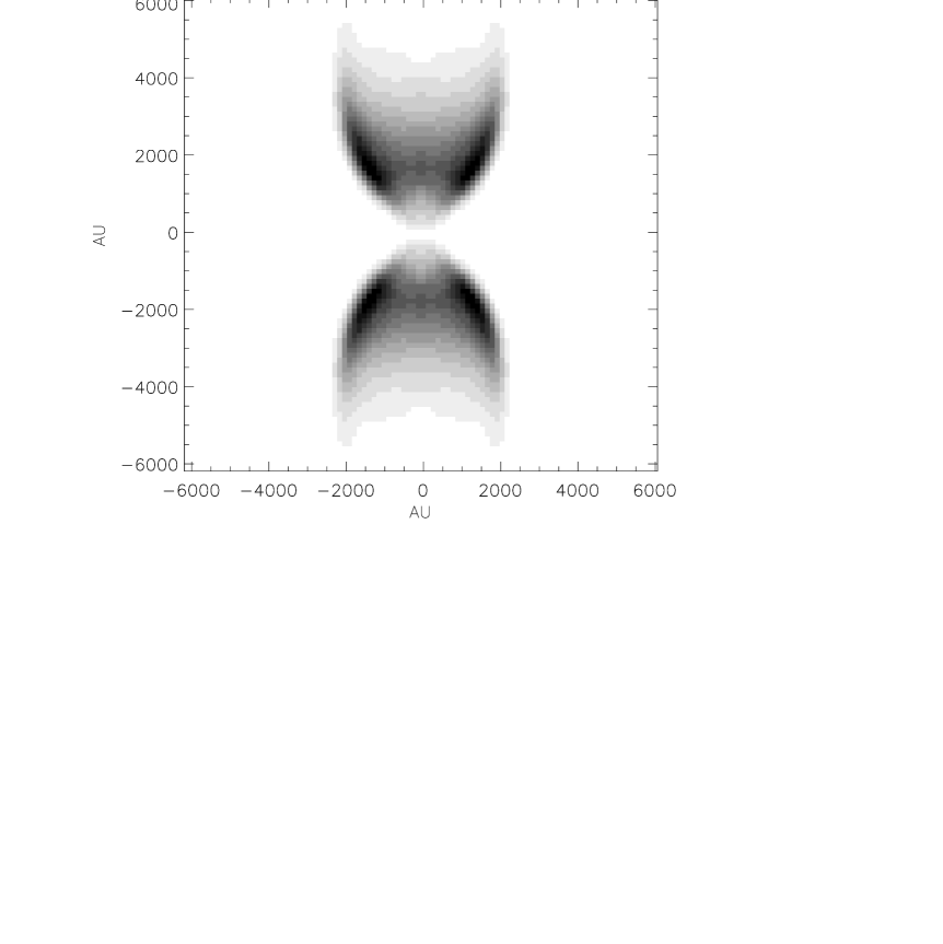
Figure 1: Linear greyscale representation of HCO${}^{+}~{}(1-0)$ best model. The peak of the emission is $5.2~{}{\rm K~{}km~{}s^{-1}}$. The viewing angle is $0\deg$

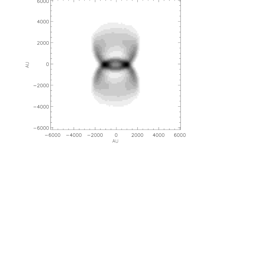
Figure 2: Linear greyscale representation of HCO${}^{+}~{}(1-0)$ best model. The peak of the emission is $7.0~{}{\rm K~{}km~{}s^{-1}}$. The viewing angle is $60\deg$

For the best fit model we have also considered the possibility of temperature variations along the boundary layer. We assumed that the temperature varies in a similar manner to the HCO⁺ abundance variation in (ii). This would seem plausible if both the HCO⁺ enhancement and the excess heating arise from shock activity. Thus, we again made the assumption that the shock activity and hence temperature is inversely proportional to the radius of curvature, and is normalised so that it lies in the range 10–100K. The effect on the overall morphology of the emission is much less marked than the effect of varying the HCO⁺ abundance and does not even have very strong effects of the 1$\to 0:3\to 2:4\to 3$ line ratios. Therefore, to simplify the analysis, the best fit model whose results we present here is one in which the temperature is kept constant along the boundary layer.

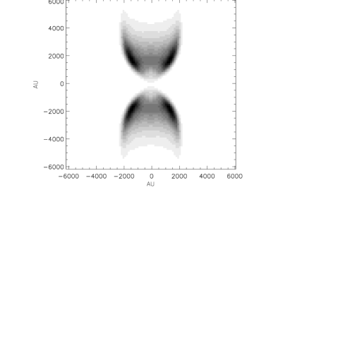
Figure 3: Linear greyscale representation of HCO${}^{+}~{}(3-2)$ best model. The peak of the emission is $0.74~{}{\rm K~{}km~{}s^{-1}}$. The viewing angle is $0\deg$

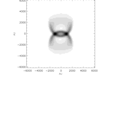
Figure 4: Linear greyscale representation of HCO${}^{+}~{}(3-2)$ best model. The peak of the emission is $1.3~{}{\rm K~{}km~{}s^{-1}}$. The viewing angle is $60\deg$

Figures 1 to 6 all show results from the same (‘best fit’) model, but for different transitions and viewing angles. Figure 1 shows a grayscale representation of the integrated line intensity for the HCO⁺(1$\to$0) line. For this particular calculation, the viewing angle is 0^∘ (i.e. the outflow is in the plane of the sky, so that the viewing angle is perpendicular to the axis of the jet). Very similar results are obtained for the $3\to 2$ and $4\to 3$ transitions. Note the lack of emission close to the origin of the flow, consistent with the observations and essentially a result of the fact that the curvature of the flow - and hence the implied shock activity and chemical enrichment - vanish at the origin. Note also the strongly limb-brightened emission from the edges of the cavity. Again, the thickness, shape (including the location of the peaks of the emission) and intensity contrast match the observations well.

The model emission compares very well with the observations, given the uncertainties dues to the collision rates, as discussed in Section 2. Hogerheijde et al. (1998) measure an integrated intensity in the HCO⁺(1$\to$0) line of $<2.0~{}{\rm K~{}km~{}s^{-1}}$ over their $5\arcsec$ beam. The peak emission for the best fit model, as displayed in Figure 1, is $5.4~{}{\rm K~{}km~{}s^{-1}}$ over a $1.5\arcsec$ beam and when this model is convolved to a $5\arcsec$ beam, the peak emission becomes $3.2~{}{\rm K~{}km~{}s^{-1}}$ (since the emission is concentrated in the bright boundary layer).

Figure 2 also shows a grayscale map of the integrated line intensity for the $3\to 2$ line, but in this case for a tilted (60^∘) viewing angle. Figures 3 and 4 show greyscale maps of the integrated line intensity for the HCO⁺(3$\to 2$) line for different viewing angles (0^∘ and 60^∘).

Figure 5 gives a grid map of the spectral line profiles for the HCO⁺($1\to 0$) line for an assumed viewing angle of 0^∘. Again, similar results are obtained for both the ($3\to 2$) and the ($4\to 3$) line maps. At the extreme edges of the cavity/boundary layer the lines of sight essentially intercept the boundary layer cone at one point with a relatively long path length through the boundary layer - hence the single peaked, limb-brightened emission. Along other lines of sight (and most strongly along lines of sight that intercept the outflow axis) the path intercepts the boundary layer cone at two points; the near side (which is approaching the observer) and the far side (which is receding) - hence the double peaked emission. The separation of the peaks (and the difference between the projected line of sight velocities of the two components) falls as one moves away from the outflow axis.

Figure 6 gives a grid map of profiles for the HCO⁺($1\to 0$) line and a viewing angle of 60^∘. Note that the line profiles are qualitatively quite different to those shown in fig. 5. With the outflow axis tilted out of the plane of the sky, the whole of the lower outflow lobe is tilted towards the observer, whilst the upper lobe is tilted away from the observer. As a consequence the line profiles show a net redshift/blueshift in the upper/lower lobes.

Most interestingly, there is some rather complex behaviour close to the origin; the line profiles are asymmetric and self-reversed, but along some lines of sight the red wing is stronger than the blue, whilst along other, nearby, lines of sight the opposite is true. Bearing in mind the inclination (60^∘) of the source this is an effect of observing parts of the flow that are receding and parts that are approaching the observer along the line of sight. Looking near the centre of the bipolar flow, the line of sight intersects more than one surface of the bipolar cones. This observation does, however, emphasize that it is very difficult to interpret single line profiles in the context of inflows/outflows without a clear depiction of the large scale dynamics of the system. As an extreme example, an observer whose sole observation was a high resolution observation along one of the lines of sight which yields a blue$>$red double peaked asymmetry could be misled into believing that the source is undergoing systemic infall.

5 Discussion and Conclusions

In this study we have concentrated on the implications of the radiative transfer modelling for our understanding of the chemical structure of bipolar outflow jet/boundary layers. We have not attempted to present or test a dynamical model of any sophistication. This is in contrast with some previous studies (e.g. Hogerheijde, 1998; Lee et al., 2000; Arce and Goodman, 2002) which have considered the hydrodynamic activity in the jet, boundary layer and surrounding cloud in some detail. Instead, although we do not constrain the hydrodynamics of the flow, our study makes some important conclusions concerning the origin and level of anomalous chemical activity within boundary layers, and how - using a state-of-the-art radiative transfer code - high resolution observations can be used to diagnose that activity.

In his study, Hogerheijde (1998) utilized an axisymmetric non-LTE Monte-Carlo to study a boundary layer whose thickness is 1/5 of the total width of the (evacuated) jet cavity. His model of the boundary layer was based on a plausible Couette flow in which the density, flow velocity and temperature vary across the boundary layer in simple monotonic fashions, maintaining pressure balance at all points (Stahler, 1994). Whilst somewhat more sophisticated than our uniform density flow, the model had problems in reproducing the observed morphology of L1527 - and in particular the density contrast between the limb-brightened edges and the body of the outflow cavity. Indeed, reasonable fits to the observed morphology - the line intensities and spatial contrasts in L1527 - were only obtained if the HCO⁺ abundance in the boundary layer is not enhanced over that in the envelope, but the fractional ionization in the boundary layer is very high [X(e^-)$\sim 10^{-4}$].

Figure 5: Line profiles of HCO${}^{+}~{}(1-0)$ for the best model. For clarity, a subset of the 96x96 array of line profiles is displayed: only the central regions are shown and only every fourth profile, in both X and Y directions, is displayed. The viewing angle is $0\deg$. The tiny peaks of emission are from the cold envelope gas

Figure 6: Line profiles of HCO${}^{+}~{}(1-0)$ for the best model. For clarity, a subset of the 96x96 array of line profiles is displayed: only the central regions are shown and only every fourth profile, in both X and Y directions, is displayed. The viewing angle is $60\deg$. The tiny peaks of emission are from the cold envelope gas

We do not reproduce this result, and in particular we do not find that by raising the HCO⁺ abundance in the boundary layer that the cavity ‘fills’ due to increased opacity. What we do find is that the density and contrast are more sensitive to the adopted HCO⁺ abundance enhancement and the thickness of the boundary layer, whilst the detailed morphology is dependent on the assumed outflow shape. In any case we do not find that such an extreme level of ionization is necessary. Indeed, it is not clear what the source of such a high level of ionization would be. More importantly, it must be remembered that the dominant loss route of HCO⁺ in dark clouds is dissociative recombination, so it would seem reasonable to expect a significant suppression of HCO⁺ if X(e^-)$\sim 10^{-5}-10^{-4}$.

Our study is more restricted to a chemical analysis of the interface and thus adopts a much simpler dynamical model. Our modelling has attempted to reproduce the cross-shaped emission seen in L1527 (and other sources) with the appropriate intensity contrasts in the outflow lobes. The cause of the brightness in the cross-arms is essentially due to limb-brightening effects. Clearly, if the boundary layer is too thick then significant emission will be apparent along all lines of sight which pass through the boundary layer, and the morphology would tend to look more like a ‘bow tie’ rather than a hollow cross.

Our tanh geometry is somewhat arbitrary, but was chosen because it matches well the observed morphology. The level of HCO⁺ enhancement and our plausible explanation of its correlation with the shape of the outflow then yields patterns of intensity that closely resemble the high resolution maps; in particular the strong enhancements (and the location of the peaks of emission) in the limb-brightened wings, a natural explanation for the limited extent of the emission and the lack of emission close to the origin.

The essential findings of this paper therefore are:

1. A strong enhancement of the HCO⁺ abundance is required in the boundary layer between the outflow jet and the surrounding molecular core in order to explain the observations of certain outflow sources associated with star-forming cores

2. We have proposed a plausible, if simple, mechanism by which this enhancement can occur with the observed morphologies and contrasts; shock liberation and photoprocessing of molecular material stored in icy mantles. The degree of shock activity is closely related to the morphology of the source

3. We have shown how asymmetric, double-peaked line profiles can be generated with strong spatial variations in the relative strength of the red and blue wings.

References

- (1) Arce H. G., Goodman A. A., 2001, ApJ, 554, 132
- (2) Arce H. G., Goodman A. A., 2002, ApJ, 575, 928
- (3) Bachiller R., Guilloteau S., Dutrey A., et al., 1995, A&A, 299, 857
- (4) Flower D. R., 1999, MNRAS, 305, 651
- (5) Hogerheijde M. R., 1998, PhD Thesis, University of Leiden
- (6) Hogerheijde M. R., van Dishoeck E. F., Blake G. A., van Langevelde H. J., 1997, ApJ, 489, 293
- (7) Hogerheijde M. R., van Dishoeck E. F., Blake G. A., van Langevelde H. J., 1998, ApJ, 502, 315
- (8) Keto E., 1990, ApJ, 355, 190
- (9) Keto E., Bergin E., Rybicki G., Plume R., 2003, ApJ, submitted
- (10) Lee C.-F., Mundy L. G., Reipurth B., Ostriker E. C., Stone J. M., 2000, ApJ, 542, 925
- (11) Lee C.-F., Mundy L. G., Stone J. M., Ostriker E. C., 2002, ApJ, 576, 294
- (12) Lim A. J., Rawlings J. M. C., Williams D. A., 2001, A&A, 376, 336
- (13) Marti F., Noerdlinger P. D., 1977, ApJ, 215, 247
- (14) Raga A., Cabrit S., 1993, A&A, 278, 267
- (15) Rawlings J. M. C., Hartquist T. W., 1997, ApJ, 487, 672
- (16) Rawlings J. M. C., Taylor S. D., Williams D. A., 2000, MNRAS, 313, 461
- (17) Rybicki G. B., Hummer D. G., 1978, ApJ, 219, 654
- (18) Rybicki G. B., Hummer D. G., 1991, A&A, 245, 171
- (19) Shu, F., Ruden S. P., Lada C. J., Lizano S., 1991, ApJ, 370, L31
- (20) Spaans M., Hogerheijde M. R., Mundy L. G., van Dishoeck E. F., 1995, ApJ, 455, L167
- (21) Stahler, S. W., 1994, ApJ, 422, 616
- (22) Velusamy T., Langer W. D., 1998, Nature, 392, 685
- (23) Viti S., Natarajan S., Willliams D. A., 2002, MNRAS, 336, 797
- (24) Young L. M., Keto E., Ho P. T. P., 1998, ApJ, 507, 270
- (25) Zhou S., Evans N. J. II, Kömpe C., Walmsley C. M., 1993, ApJ, 404, 232
- (26) Zhou S., Evans N. J. II, Wang Y., Peng R., Lo K. Y., 1994, ApJ, 433, 131