Temperature distribution in magnetized neutron star crusts

We investigate the influence of different magnetic field configurations on the temperature distribution in neutron star crusts. We consider axisymmetric dipolar fields which are either restricted to the stellar crust, “crustal fields”, or allowed to penetrate the core, “core fields”. By integrating the two-dimensional heat transport equation in the crust, taking into account the classical (Larmor) anisotropy of the heat conductivity, we obtain the crustal temperature distribution, assuming an isothermal core. Including quantum magnetic field effects in the envelope as a boundary condition, we deduce the corresponding surface temperature distributions. We find that core fields result in practically isothermal crusts unless the surface field strength is well above $10^{15}$ G while for crustal fields with surface strength above a few times $10^{12}$ G significant deviations from isothermality occur at core temperatures inferior or equal to $10^{8}$ K. At the stellar surface, the cold equatorial region produced by the quantum suppression of heat transport perpendicular to the field in the envelope, present for both core and crustal fields, is significantly extended by the classical suppression at higher densities in the case of crustal fields. This can result, for crustal fields, in two small warm polar regions which will have observational consequences: the neutron star has a small effective thermally emitting area and the X-ray pulse profiles are expected to have a distinctively different shape compared to the case of a neutron star with a core field. These features, when compared with X-ray data on thermal emission of young cooling neutron stars, will open a way to provide observational evidence in favor, or against, the two radically different configurations of crustal or core magnetic fields.

1 Introduction

The presence of strong magnetic fields in neutron stars is one of their distinctive characteristics. In typical neutron stars the observed and/or inferred surface fields are of the order of $10^{12...13}$ G ; for magnetars they even reach $10^{14...15}$ G. The strength, structure and time evolution of the magnetic field is intimately related to its origin, which is still an open problem. Basically, two qualitatively different types of field structures are conceivable, one having an initial field penetrating the whole star while the other is characterized by having the field and its supporting currents restricted to the stellar crust (see, e.g., Chanmugam C92 (1992)). To date, there is still no compelling observational evidence in favor of or against either of these two hypotheses but recently Link L03 (2003) argued that long period pulsar precession, as observed in PSR B1828-11 (Stairs et al. SLS00 (2000)), may be impossible if the magnetic field penetrates regions of the core where neutrons are superfluid and proton superconducting.

Any observed magnetic field, either based on crustal or core currents, has to penetrate the crust matter, thereby affecting its transport properties. Moreover, the structure of the field in the shallow spherical shell layer below the surface has a direct effect on the surface temperature and leads to a non-uniform distribution with observational consequences (Page P95 (1995)) if its strength is above $10^{10}$ G. Roughly, the effects of the magnetic field onto the transport processes can be divided into classical and quantum ones (see, e.g., Yakovlev & Kaminker YK94 (1994) for a review). The classical effects are due to the Larmor rotation of the electrons, the main carriers of charge and heat, and are determined by the magnetization parameter $\omega_{\scriptscriptstyle B}\tau$ where $\omega_{\scriptscriptstyle B}\equiv eB/m_{e}^{*}c$ is the gyrofrequency of the electrons, $\tau$ being their relaxation time and $m_{e}^{*}$ their effective mass. Quantized motion of the electrons transverse to the magnetic field causes the quantum effects which are of importance only if few Landau levels are occupied, requiring thus densities $\rho<\rho_{B}=7045(B/10^{12}\mathrm{G})^{3/2}\frac{<A>}{<Z>}$ g cm^-3 and temperatures $T\ll T_{B}\approx 1.34\cdot 10^{8}(B/10^{12}\mathrm{G})$ K (Potekhin et al. PYCG03 (2003)) where $<A>$ and $<Z>$ are the average mass and charge numbers of the ions. From these numbers it becomes clear that quantum effects will play an important role for strong magnetic fields in the outermost layers of the neutron star crust - the thin low density shell of the envelope - but are negligible in the deeper layers. The thinness of this envelope justifies a study of heat transport in a plane parallel, one dimensional approximation and many such calculations have been performed (see, e.g., for the most recent one, Potekhin & Yakovlev PY01 (2001), hereafter PY01, and references therein). Two-dimensional calculations of heat transport with magnetic field have been presented by Schaaf (1990a ,1990b ) who however restricted himself to the thin envelope and an uniform magnetic field. Tsuruta (T98 (1998)) has presented results of two-dimensional cooling calculations of neutron stars which included the quantizing effect of a dipolar magnetic field in the envelope. These 2D calculations showed that the 1D approximation is indeed very good when the field affects heat transport only in the thin envelope.

The deeper layers of the crust can, however, be affected by classical effects in case of strong fields, i.e., large $\omega_{\scriptscriptstyle B}$, and/or low temperature, i.e., high $\tau$. In such a case the usual assumption of an isothermal crust is questionable and this is the issue we want to address in this paper. In particular, in the case of a crustal magnetic field its strength in the crust unavoidably exceeds its surface value by one to two orders of magnitude (see, e.g., Page et al. PGZ00 (2000))  and its effect can naturally be expected to be stronger than in the case of a field permeating the whole star. This may open a way to study the structure of the magnetic field in the crust and provide observational features which will allow us to discriminate between the above mentioned two types of hypothesized field structure, crustal vs. core.

The paper is organized as follows: In the next Sect.  2 the basic equations are introduced which describe the magnetic field and the heat transport influenced by it. The components of the heat conductivity tensor are given and the outer boundary condition is discussed. The physical input as well as the numerical method are shortly described. In Sect. 3 the results of the numerical calculations are presented. For different core temperatures, magnetic field strengths and geometries the crustal temperature profiles, the surface temperature distributions and the corresponding luminosities are calculated. Sect. 4 is devoted to the discussion of the consequences of the magnetic field effects on to the crustal and surface temperature distribution.

2 Physics Input

2.1 Heat transport and magnetic field

The thermal evolution of the crust is determined by the energy balance equation

$$C\,\frac{\partial T}{\partial t}=\mathrm{Sources}-\mathrm{Sinks}-\@vec{\nabla}\cdot\@vec{F}$$ (1)

and the heat transport equation

$$\@vec{F}=-\hat{\kappa}\cdot\@vec{\nabla}T$$ (2)

where $C$ denotes the specific heat per unit volume, $\@vec{F}$ is the heat flux density and $\hat{\kappa}$ the tensor of heat conductivity.

In this paper we intend to consider only the effect of the crustal magnetic field on to the stationary temperature distribution in the crust, which, in a first approximation, is assumed to be free of heat sources and sinks. The cooling process itself as well as the back reaction of the now non-spherically symmetric temperature distribution on to the magnetic field decay will be beyond the scope of this work.

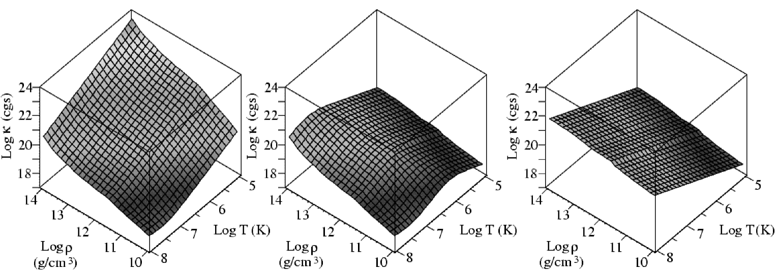
Figure 1: Thermal conductivity $\kappa_{0}$, in cgs units, versus density $\rho$ and temperature $T$. The left panel shows the phonon-only contribution $\kappa_{0\;\rm ph}$, the right one the impurity-only contribution $\kappa_{0\;\rm imp}$, and the central panel the complete $\kappa_{0}$ (with an impurity concentration $Q_{\mathrm{imp}}=0.1$).

In the relaxation time approximation the components of $\hat{\kappa}$ parallel and perpendicular to the magnetic field, $\kappa_{\|}$ and $\kappa_{\perp}$ respectively, as well as the Hall component, $\kappa_{\wedge}$, are related to the scalar heat conductivity $\kappa_{0}$ and to the magnetization parameter $\omega_{\scriptscriptstyle B}\tau$ by (Yakovlev & Kaminker YK94 (1994))

$$\kappa_{\|}=\kappa_{0}\,,\quad\kappa_{\perp}=\frac{\kappa_{0}}{1+(\omega_{\scriptscriptstyle B}\tau)^{2}}\,,\quad\kappa_{\wedge}=\omega_{\scriptscriptstyle B}\tau\,\kappa_{\perp}$$ (3)

For $\kappa_{0}$ we use

$$\kappa_{0}=\frac{\pi^{2}k_{B}^{2}Tn_{e}}{3m_{*}\nu}$$ (4)

where $\nu=1/\tau$ is the effective electron collisional frequency and is given by the sum

$$\nu=\nu_{\mathrm{ph}}+\nu_{\mathrm{ion}}+\nu_{\mathrm{imp}}$$ (5)

where $\nu_{\mathrm{ph}}$ is the effective collisional frequency for electron-phonon, $\nu_{\mathrm{ion}}$ for electron-ion, and $\nu_{\mathrm{imp}}$ for electron-impurity collisions. Since for the range of densities and temperatures we are interested in the crust is always in the solid state we neglect $\nu_{\mathrm{ion}}$ and for $\nu_{\mathrm{ph}}$ we use the calculations Baiko & Yakovlev (BY96 (1996)) while we take $\nu_{\mathrm{imp}}$ from Yakovlev & Urpin (YU80 (1980)). Everywhere in this work we assume an “impurity parameter” $Q\equiv x_{\mathrm{imp}}\overline{(\Delta Z)^{2}}$ equal to 0.1, where $x_{\mathrm{imp}}$ is the fractional number of impurities which have a mean square charge excess of $\overline{(\Delta Z)^{2}}$. Figure 1 shows the resulting $\kappa_{0}$: note that $\nu_{\mathrm{imp}}$ is almost temperature independent while $\nu_{\mathrm{ph}}$ scale approximately as $T^{2}$ so that if $\nu=\nu_{\mathrm{ph}}$ then the “phonon-only conductivity” $\kappa_{0\;\mathrm{ph}}$ $\sim T^{-1}$ (Fig. 1 left panel) but if $\nu=\nu_{\mathrm{imp}}$ we would have an “impurity-only conductivity” $\kappa_{0\;\mathrm{imp}}$ $\sim T^{+1}$ (Fig. 1 right panel) and the exact $\kappa_{0}$ (Fig. 1 central panel), which one could write as $\kappa_{0}=(1/\kappa_{0\;\mathrm{ph}}+1/\kappa_{0\mathrm{imp}})^{-1}$, shows both types of behaviours depending on which type of collision process dominates.

The magnetization parameter $\omega_{\scriptscriptstyle B}\tau$ varies strongly throughout the crust by many orders of magnitude. In $\omega_{\scriptscriptstyle B}$ both $B$ and $m_{e}^{*}$ span a large range of values throughout the crust and in $\tau$ there is also a strong dependence on the temperature $T$, chemical composition and the thermodynamic phase of the matter. For illustration we show, in Fig. 2, $\omega_{\scriptscriptstyle B}\tau$ in the crust at various uniform temperatures and a uniform field strength: however, neither $T$ nor $B$ will be uniform in our realistic calculation presented below. Note that values of $\omega_{\scriptscriptstyle B}\tau$ at $T=10^{5}$ and $10^{6}$ K are very close to each other because at such low $T$ $\nu$ is dominated by $\nu_{\mathrm{imp}}$ which is temperature independent while when going to increasingly higher temperatures $\nu_{\mathrm{ph}}$ contributes more and more and hence $\tau$ decreases. Finally, Fig. 3 shows the resulting $\kappa_{\perp}$’: notice its very different $T$–$\rho$ behaviour compared to $\kappa_{0}$ due to the simple fact that at high $\omega_{\scriptscriptstyle B}\tau$ we obtain $\kappa_{\perp}\propto\tau^{-1}$ while $\kappa_{0}\propto\tau$.

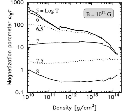
Figure 2: Magnetization parameter $\omega_{\scriptscriptstyle B}\tau$ vs. density at six different temperatures (as labeled on the curves) assuming a uniform magnetic field of strength $B=10^{12}$ G. Its value for different field strengths scales linearly in $B$.

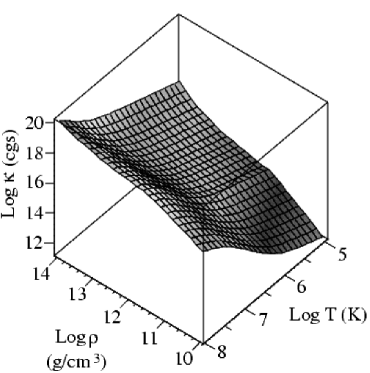
Figure 3: Thermal conductivity, in cgs units, perpendicular to the magnetic field, $\kappa_{\perp}$, vs. density $\rho$ and temperature $T$ for a uniform magnetic field of strength $3\times 10^{12}$ G. For field strengths $\gg 10^{12}$ G, i.e., for $\omega_{\scriptscriptstyle B}\tau\gg 1$, $\kappa_{\perp}$ scales as $B^{-2}$. The impurity parameter $Q$ is assumed to be 0.1.

2.2 The Crustal Magnetic Field

A dipolar poloidal magnetic field can be conveniently described in terms of the (possibly time dependent) Stoke’s stream function $S=S(r,t)$. The vector potential $\@vec{A}=(0,0,A_{\varphi})$ is written as $A_{\varphi}=S(r,t)\sin\theta/r$, where $r$, $\theta$ and $\varphi$ are spherical coordinates. The field components are then expressed as

$$B_{r}=+\frac{2\cos\theta}{r^{2}}S(r,t)=B_{0}\;\frac{\cos\theta}{x^{2}}\;s(x,t)$$ (6)

$$B_{\theta}=-\frac{\sin\theta}{r}\frac{\partial S(r,t)}{\partial r}=-\frac{B_{0}}{2}\;\frac{\sin\theta}{x}\;\frac{\partial s(x,t)}{\partial x}$$ (7)

$$B_{\varphi}=0$$ (8)

where $B_{0}$ is the field strength at the magnetic pole, and we have introduced normalized variables $S=sB_{0}R_{N\!S}^{2}/2$, with $s=1$ at the magnetic north pole, and $x=r/R_{N\!S}$. The vacuum solution, outside the star, is simply $s=1/x$. At the surface, $x=1$, the standard boundary condition for matching to a vacuum dipole field should be fulfilled,

$$\frac{\partial S}{\partial r}+\frac{S}{R_{N\!S}}=0\;\;\;\;\;\mathrm{i.e.}\;\;\;\;\;\left.\frac{\partial s}{\partial x}\right|_{x=1}=-s$$ (9)

and at the center regularity requires $S(r=0,t)\equiv 0$.

For the present investigation we select for the crustal field configuration a snapshot of the evolution of $S(x,t)$. The Stoke’s function $S(x,t)$ was calculated by solving the induction equation, applying the above boundary conditions and an electric conductivity which reflects the same microphysics as the heat conductivity does for the model under consideration (see, e.g., Geppert & Urpin GU94 (1994) or Page et al. PGZ00 (2000)).

Figure 4: Magnetic field lines of the core field (left panel) and of the crustal field as applied in our calculations. Both field configurations match for $r\geq R_{NS}$ with a dipolar poloidal vacuum field. They are presented in a meridional plane, of the crust for $\rho_{n}\geq\rho\geq\rho_{b}$ (see Sects.  2.4 and  2.5). The polar surface value $B_{0}$ is identical for both field types.

The initial value $S(x,t=0)$ is a priori unknown and depends on the field generation process. For a crustal magnetic field, the function $S(x,t=0)$ initially vanishes in the core and, due to proton superconductivity, the Meissner-Ochsenfeld effect prevents the field from penetrating into the core (see, e.g. Page et al. PGZ00 (2000)). A typical crustal field structure is shown in the right panel of Fig. 4. In case the magnetic field is maintained by electric currents circulating in the core the field penetrates the crust too but has a qualitatively different structure. Let us assume that for the core field there are no currents in the crust and the field is maintained in the core by axisymmetric currents circulating around the center of the star. Then a dipolar field will penetrate the crust with the components

$$B_{r}^{dipole}=B_{0}\;\frac{\cos\theta}{x^{3}}\;,$$ (10)

$$B_{\theta}^{dipole}=\frac{B_{0}}{2}\;\frac{\sin\theta}{x^{3}}\;,$$ (11)

$$B_{\varphi}^{dipole}=0\;,$$ (12)

where $B_{0}$ denotes again the polar surface value of the magnetic field. The crustal field lines of such a field are presented in the left panel of Fig. 4. A comparison of the geometries of both fields immediately suggests that the star-centered core field will not significantly affect the heat transport through the crust while a crustal field may cause drastic changes. Moreover, in the crust $B_{\theta}$ has to be much larger than $B_{\theta}^{dipole}$, for a given identital external field, since the flux of a crustal field is compressed into a layer of thicknes $\Delta r\sim\frac{1}{10}-\frac{1}{20}$ of $R_{N\!S}$, while the flux of a core field can expand within the whole core, i.e., typically $B_{\theta}\sim 10-20B_{\theta}^{dipole}$.

2.3 The Two-Dimensional Heat Transport Equation

Denoting the components of the temperature gradient $\@vec{\nabla}T$ parallel and perpendicular to the unit vector of the magnetic field, $\@vec{b}$ as well as the Hall, component by

$$(\@vec{\nabla}T)_{\|}=\@vec{b}\;(\@vec{\nabla}T\cdot\@vec{b})\;\; \;\;(\@vec{\nabla}T)_{\perp}=\@vec{b}\times(\@vec{\nabla}T\times\@vec{b})\;\;,$$ , (13)

$$(\@vec{\nabla}T)_{\wedge} = \@vec{b}\times\@vec{\nabla}T\;\;,$$

the magnetic–field–influenced heat flux can be expressed by

$$\hat{\kappa}\cdot\@vec{\nabla}T=$$

$$\kappa_{\|}\;\@vec{b}\;(\@vec{\nabla}T\cdot\@vec{b})+\kappa_{\perp}\;\@vec{b}\times(\@vec{\nabla}T\times\@vec{b})+\kappa_{\wedge}\;\@vec{b}\times\@vec{\nabla}T\;\;.$$ (14)

This provides the following expression for the heat flux in terms of the scalar heat conductivity, the magnetization parameter, the temperature gradient and the unit vector of the magnetic field:

$$\@vec{F}=-\hat{\kappa}\cdot\@vec{\nabla}T=-\;\frac{\kappa_{0}}{1+(\omega_{\scriptscriptstyle B}\tau)^{2}}\times$$

$$\left[\@vec{\nabla}T+(\omega_{\scriptscriptstyle B}\tau)^{2}\;\@vec{b}\;(\@vec{\nabla}T\cdot\@vec{b})+\omega_{\scriptscriptstyle B}\tau\;\@vec{b}\times\@vec{\nabla}T\right]\,\,.$$ (15)

The last term on the r.h.s. represents the Hall component of the heat flux. Its divergence vanishes as long as the magnetic field and the temperature gradient are assumed to be axially symmetric, i.e., do not depend on the azimuthal angle $\varphi$. By use of the representation of the dipolar magnetic field in terms of the Stoke’s stream function $s$ and its radial derivatives (see Eqs. 6, 7) and by introducing the heat conductivity coefficients

$$\chi_{1}=\frac{\kappa_{0}}{1+(\omega_{\scriptscriptstyle B}\tau)^{2}}\,\,,\,\,\chi_{2}=\frac{\kappa_{0}\,(\omega_{\scriptscriptstyle B_{0}}\tau)^{2}}{1+(\omega_{\scriptscriptstyle B}\tau)^{2}}\,\,,$$ (16)

the radial and meridional components of the magnetic–field–dependent heat flux have the following form:

$$F_{x}=-\chi_{1}\frac{\partial T}{\partial x}+$$

$$\chi_{2}\left(\frac{\partial T}{\partial\theta}\frac{s}{2x^{4}}\frac{\partial s}{\partial x}\sin{\theta}\cos{\theta}-\frac{\partial T}{\partial x}\frac{s^{2}}{x^{4}}\cos^{2}{\theta}\right)\,\,,$$ (17)

$$F_{\theta}=-\chi_{1}\frac{1}{x}\frac{\partial T}{\partial\theta}+$$

$$\chi_{2}\left(\frac{\partial T}{\partial x}\frac{s}{2x^{3}}\frac{\partial s}{\partial x}\sin{\theta}\cos{\theta}-\frac{\partial T}{\partial\theta}\frac{1}{4x^{3}}\left(\frac{\partial s}{\partial x}\right)^{2}\sin^{2}{\theta}\right)\,\,,$$ (18)

where $T$ is measured in units of $T_{\mathrm{core}}$ and the heat flux is normalized on $T_{\mathrm{core}}/R_{N\!S}$. Note that in Eq. 16 the magnetization parameter $\omega_{\scriptscriptstyle B_{0}}\tau$ is calculated by use of the polar surface field strength $B_{0}$.

Axial symmetry implies that, along the polar axis, $F_{\theta}$ and $\partial F_{\theta}/\partial\theta$ vanish while $x^{2}F_{x}$ is constant. Mirror symmetry at the magnetic equator implies that $F_{\theta}$ vanishes (but $\partial F_{\theta}/\partial\theta$ can be very large).

Our aim in this paper will be to find stationary solutions for the temperature distribution in the neutron star crust, i.e. to solve the equation

$$\@vec{\nabla}\cdot\@vec{F}=\frac{1}{x^{2}}\frac{\partial(x^{2}F_{x})}{\partial x}+\frac{1}{x\sin\theta}\frac{\partial(\sin\theta F_{\theta})}{\partial\theta}=0\;\;.$$ (19)

The boundary condition for this equation at the crust-core boundary is “ $T$ fixed and uniform ” and at the surface it as discussed in the following subsection.

2.4 Outer boundary: $T_{b}(\@vec{B})-T_{s}(\@vec{B})$ relationship

In the lowest–density layers, close to the surface, matter is no longer degenerate and the magnetic field affects the equation of state. Appropriate treatment of this layer requires solving for hydrostatic equilibrium simultaneously with heat transport. To avoid this problem, we separate this layer, called envelope, from the crust and incorporate it in the outer boundary condition. We stop the integration at an outer boundary density $\rho_{b}$, at radius $r_{b}$, and, for each latitude $\theta$, obtain a radial flux $F_{r}(\rho_{b},\theta)$ and a temperature $T(\rho_{b},\theta)$ which we match to the envelope. In the envelope approximation, a surface temperature $T_{s}$, and hence an out coming flux $F^{\mathrm{env}}\equiv\sigma T_{s}^{4}$, is chosen and hydrostatic equilibrium and heat transport are solved toward increasing densities up to $\rho_{b}$ giving the temperature $T^{\mathrm{env}}_{b}$ at that density. Varying $T_{s}$ gives a “$T_{b}-T_{s}$ relationship”. The matching of the envelope with our interior calculation is simply obtained by imposing $T^{\mathrm{env}}_{b}=T(\rho_{b},\theta)$ and $F^{\mathrm{env}}\equiv\sigma T_{s}^{4}=F_{r}(\rho_{b},\theta)$ which is our outer boundary condition. The magnetic field strongly affects the structure and transport properties of the envelope and the “$T_{b}-T_{s}$ relationship”: at each point $(r_{b},\theta)$ we apply an envelope with a magnetic field $\@vec{B}$ equal to the field we have at that point, hence giving us a $T_{b}(\@vec{B})-T_{s}(\@vec{B})$ relationship.

Many calculations of magnetized envelopes have been presented and we use the latest and most accurate one from PY01. These authors pose the bottom of the envelope at the neutron drip density, i.e., $\rho_{b}\approx 4\cdot 10^{11}$ g cm^-3, while we intend to apply lower values down to $\rho_{b}=10^{10}$ g cm^-3 in order to extend the 2–dimensional transport calculation as far as possible while still being safely in the non-quantizing regime. Since the temperature profile in the 1–dimensional envelope calculations of Potekhin & Yakovlev is quite flat between $4\cdot 10^{11}$ g cm^-3 and $10^{10}$ g cm^-3 the same $T_{b}-T_{s}$ relationship can be applied for the lower $\rho_{b}$ which we consider a good approximation. Explicitly, we apply their equations (26) to (30) but replace their $T_{\mathrm{core}}$ which they assume to be spherically symmetric by our calculated angle-dependent $T_{b}(\theta)$.

To illustrate the main features of this boundary condition, a good approximation (Greenstein & Hartke GH83 (1983);YP01) is to write it as

$$F_{r}(\rho_{b},\Theta_{B},B,T_{b})\approx F_{\|}\cos^{2}\Theta_{B}+F_{\perp}\sin^{2}\Theta_{B}\,\,,$$ (20)

which expresses $F_{r}$, for an arbitrary angle $\Theta_{B}$ between $\@vec{B}$ and the radial direction, in terms of the radial flux for a radial field $F_{\|}\equiv F_{r}(\rho_{b},\Theta_{B}=0,B,T_{b})$ and for a meridional field $F_{\perp}\equiv F_{r}(\rho_{b},\Theta_{B}=\pi/2,B,T_{b})$. For a dipolar field $\Theta_{B}$ is related to the polar angle $\theta$ by $\tan\Theta_{B}=0.5\tan\theta$. Note that when $B\gg 10^{11}$ G one has $F_{\perp}\ll F_{\|}$, i.e., the envelope is blanketing the star much more strongly around the magnetic equator than around the poles.

2.5 Equation of state and chemical composition

We will consider a $1.4M_{\odot}$ neutron star whose structure is obtained by integrating the Tolman-Oppenheimer-Volkoff equation of hydrostatic equilibrium. The core matter is described by the equation of state (EOS) calculated by Wiringa et al. (WFF88 (1988)). We separate the crust from the core at the density $\rho=\rho_{n}\equiv 1.62\times 10^{14}$ g cm^-3 (Lorenz et al. LRP93 (1993)) and use the EOS of Negele & Vautherin (NV73 (1973)) for the inner crust, at $\rho>\rho_{drip}\equiv 4.4\times 10^{11}$ g cm^-3, and Haensel et al. (HZD89 (1989)) for the outer crust. We assume that the chemical composition is that of cold catalyzed matter, as is the case for these two crustal EOSs.

The star so produced has a radius $R_{NS}=10.9$ km and the crust-core boundary is at radius $r_{n}=0.925R_{NS}=9.33$ km.

2.6 Numerical method

Figure 5: The crustal temperature $T$ (normalized on $T_{\mathrm{core}}$) as a function of the density within the crust at 4 different polar angles: $\theta=0$: dotted-dashed line (almost coincident with the upper limit of the figure), $\theta=30$: dashed line, $\theta=60^{0}$: dotted line, and $\theta=90^{0}$: full line, for a crustal field of strength $B_{0}=3\cdot 10^{12}$G. The three panels correspond, from left to right, to $T_{\mathrm{core}}=10^{8}$K, $10^{7}$K, and $10^{6}$K, respectively.

We solve the heat transport equation in its time-dependent form,

$$C\frac{\partial T}{\partial t}=-\@vec{\nabla}\cdot\@vec{F}$$ (21)

starting with constant temperature, $T=T_{\mathrm{core}}$. As boundary condition at the lower boundary the temperature is kept fixed to the value $T_{\mathrm{core}}$ at all times while at the outer boundary the radial heat flux is related to the temperature at the same point as described above. The code is then run until a stationary state is reached.

For the discretization of the spatial derivatives a staggered mesh method as described in Stone & Norman (SN92 (1992)) is used in spherical polar coordinates ($r$ and $\theta$). For the integration in time the fully explicit method turned out to be prohibitively slow because the diffusion coefficients vary strongly in space in the case of strong magnetic fields. We therefore use the scheme in an operator-split implementation that treats the radial diffusion terms implicitly while the horizontal diffusion and the ${\partial T}/\partial\theta$ term in $F_{r}$ remain explicit. This keeps the computational effort per time step small as the equations to be solved are tridiagonal, but allows for a sufficiently large time step to reach a stationary state within several hours of computing time. For the evaluation of the transport coefficients and the outer boundary condition the temperature resulting from the last time step is always used, i.e., only the radial derivatives are treated implicitly.

3 Results

3.1 Internal temperature

Figure 6: Same as Fig. 5 but for a dipolar core field with $T_{\mathrm{core}}=10^{7}$K.

The importance of the magnetic-field-induced non-isothermality of the whole crust is illustrated in Figs. 5, 6, 7, and 8. The temperature profiles of Fig. 5 when compared with Fig. 6, show clearly the difference between a crustal and a core field, the latter inducing temperature variations in the crust of much less than 1% at $B_{0}=3\cdot 10^{12}$ G while the former can result in variations of a factor two for the same dipolar external field strength and $T_{\mathrm{core}}=10^{7}$K, and even much larger at lower $T_{\mathrm{core}}$.

For strong fields, when $\omega_{\scriptscriptstyle B}\tau\gg 1$, one has $\kappa_{\|}=\kappa_{0}\gg\kappa_{\perp}$ and hence heat flows essentially along the field lines and, given the large values of $\kappa_{0}$, no large temperature gradient can build up along them, as illustrated in Fig. 7. Only extremely strong core fields may cause significant deviations from the isothermality of the crust; for $B_{0}=10^{16}$G we could observe a difference of only $10$ % for $T(\rho_{b})$ between pole and equator. The qualitative difference between core and crustal magnetic fields is then easily understood by observing that field lines are essentially radial in most of the crust in the case of a core field while they are predominantly meridional for a crustal field inhibiting radial heat flow in a large part of the crust. We could find significant differences to the isothermal crust model only if the polar surface field strength exceeds $10^{12}$G. Additionally, the core temperature should be smaller than $10^{8}$K.

In the case of a star-centered core field, Fig. 6 and the right panel of Fig. 7 shows that the stellar equator is very slightly warmer than the pole. This is a direct consequence of the outer boundary condition, i.e., the envelope: magnetic–field–induced anisotropies are weak within the crust for such fields but are large in the envelope which is more insulating around the equator than around the poles.

A 3D representation of the crust temperature is shown in Fig. 8: it may be surprising in the sense that heat flows into the crust from the core, at a fixed $T_{\mathrm{core}}$, and out of the crust at the surface and most of the heat comes out in the polar regions which are, first, warmer than the equator and where, second, the envelope is less insulating. So heat must be flowing from the equatorial regions toward the polar regions, i.e., apparently from cold regions toward warmer ones ! That this situation cannot violate the second law of thermodynamics is built into the heat conductivity tensor $\hat{\kappa}$ which is positive definite and guarantees that $\@vec{F}\cdot\@vec{\nabla}T<0$ always. Figure 9 illustrates this situation: at a point in the northern hemisphere $\@vec{\nabla}T$ is almost perpendicular to $\@vec{B}$ and $-(\@vec{\nabla}T)_{\theta}$ is clearly pointing toward the equator. However, since $F_{\|}=-\kappa_{\|}(\@vec{\nabla}T)_{\|}$, $F_{\perp}=-\kappa_{\perp}(\@vec{\nabla}T)_{\perp}$, and $\kappa_{\|}\gg\kappa_{\perp}$ we have $|F_{\|}|\gg|F_{\perp}|$ and the resulting $F_{\theta}$ is negative, i.e., pointing toward the pole: heat is flowing from the equator toward the poles but does it along the magnetic field lines from warmer regions toward colder ones. Our numerical results show that, e.g., in the northern hemisphere, $F_{\theta}$ is negative in large regions and is positive elsewhere depending on the orientation of $\@vec{B}$.

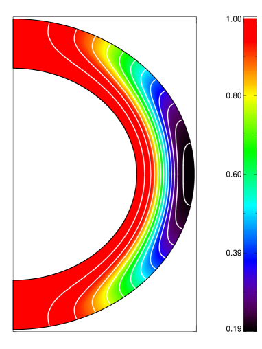
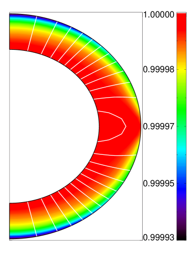
Figure 7: Representation of both field lines and temperature distribution in the crust whose radial scale ($r(\rho_{n})\leq r\leq r(\rho_{b})$) is stretched by a factor of $5$, assuming $B_{0}=3\cdot 10^{12}$G and $T_{\mathrm{core}}=10^{6}$K. Left panel corresponds to a crustal field, right panel to a star-centered core field. Bars show the temperature scales in units of $T_{\mathrm{core}}$.

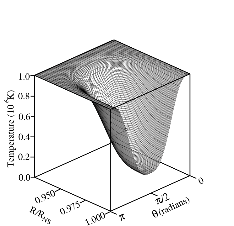
Figure 8: 3-D presentation of the temperature distribution in the crust for $T_{\mathrm{core}}=10^{6}$ K and a crustal field with strength $B_{0}=3\cdot 10^{12}$ G. (corresponding to the right panel of Fig. 5).

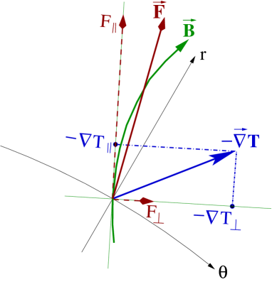
Figure 9: Illustration of the magnetic-field-induced anisotropy (see text for details)

The results shown in Fig. 5 for the crustal field configuration with the typical strength $B_{0}=3\cdot 10^{12}$G confirms the statement that with increasing magnetization parameter the anisotropy of the temperature distribution within the crust increases too. The magnetization parameter increases with increasing magnetic field strength and with decreasing crustal temperature, i.e. with decreasing $T_{\mathrm{core}}$, because the relaxation time of electron–phonon collisions grows strongly in the course of cooling. Therefore, while the temperature profile along the poles shows practically no gradient with decreasing $T_{\mathrm{core}}$ the ratio $T(\rho_{b},\theta=90^{\circ})/T(\rho_{b},\theta=0^{\circ})$ decreases from 0.95 to 0.5 and 0.2 when $T_{\mathrm{core}}$ decreases from $10^{8}$ K to $10^{7}$ and $10^{6}$ K, respectively. Also, an increase of the magnetic field strength amplifies that difference. Applying the same field structure but $B_{0}=10^{13}$G the temperature ratio becomes smaller than 0.1 for $T_{\mathrm{core}}=10^{6}$K.

Note also that the highly unknown parameter of the impurity concentration ($Q=0.1$ throughout this paper) affects the relaxation time: the more impurities the shorter the relaxation time of electron–impurity collisions. Therefore, in a very pure neutron star crust the magnetic field effects onto the crustal temperature distribution will be even more pronounced.

3.2 Surface temperature distribution

Figure 10: The surface temperature $T_{s}$ as a function of the polar angle $\theta$ and for $T_{\mathrm{core}}=10^{6}$K (left panels), $T_{\mathrm{core}}=10^{7}$K (mid panels), or $T_{\mathrm{core}}=10^{8}$K (right panels) The dashed lines show the surface temperature distribution when an isothermal crust is assumed. The full lines represent the surface temperatures when the crust temperature distributions take into account the anisotropy of heat transport induced by a crustal magnetic field (the temperature at the crust-core interface being fixed at the $T_{\mathrm{core}}$). Almost indistinguishable from the isothermal crust model is the $T_{s}$-distribution for a star-centered core field. It is shown by dot-dashed lines for $T_{\mathrm{core}}=10^{8}$K; for lower $T_{\mathrm{core}}$ the differences are even smaller. The assumed polar surface field strengths $B_{0}$ are $10^{12}$G (upper panels), $3\cdot 10^{12}$G (mid panels) and $10^{13}$G (lower panels).

The magnetic field permeating the envelope induces a non-uniform surface temperature distribution, mostly due to quantizing effects of the field at low densities, even in the case of a uniform crustal temperature (Schaaf 1990a ; 1990b ; Page P95 (1995)). The non-isothermality of the crust produced by a crustal magnetic field will result in an even more pronounced non-uniformity of the surface temperature. These effects are shown quantitatively in Fig. 10 where the two cases of core and crustal fields are compared.

The different field structures do not only affect the relation between polar and equatorial surface temperature but also the setup and the extension of the warm polar regions. In Fig. 10 it is seen that the crustal field can cause a much smaller warm polar region than a star-centered core field of the same polar surface strength would do. While for the core field geometry with $B_{0}=10^{13}$G and $T_{\mathrm{core}}=10^{8}$K the surface temperature at a polar angle of $31.5^{0}$ is reduced only to $0.93$ of its polar value, for the crustal field configuration the corresponding value is $0.82$. With decreasing $T_{\mathrm{core}}$ this difference becomes larger: thus for $T_{\mathrm{core}}=10^{6}$K the corresponding values for the core and the crustal field are $0.93$ and $0.77$, respectively. The setup of a clearly distinct warm polar region becomes more and more pronounced with an increasing magnetization parameter (i.e. increasing field strength and/or decreasing crustal temperature and/or decreasing impurity concentration) for a crustal field configuration, while the shape of the surface temperature distribution is almost unaffected by the magnetization parameter in case of a core magnetic field.

3.3 Luminosity

Having a non-uniform surface temperature distribution, $T_{s}=T_{s}(\theta)$, the effective temperature $T_{\mathrm{eff}}$ can be calculated, from its definition, as

$$4\pi R^{2}\sigma_{\scriptscriptstyle SB}T_{\mathrm{eff}}^{4}\equiv L=\int\sigma_{\scriptscriptstyle SB}T_{s}^{4}(\theta)\mathrm{d}\Sigma,$$ (22)

where $R$ is the circumferential neutron star radius and $\mathrm{d}\Sigma\equiv\sin\theta\mathrm{d}\phi\mathrm{d}\theta$ is the surface area element, so that finally the luminosity is given by

$$L=2\pi\sigma_{\scriptscriptstyle SB}R^{2}\int^{\pi}_{0}T_{s}^{4}(\theta)\sin{\theta}\mathrm{d}\theta.$$ (23)

The photon luminosities for the neutron star models under consideration with different magnetic field structures and strengths are listed in Table 1 for a model with $T_{\mathrm{core}}=10^{8}$K, Table 2 for $T_{\mathrm{core}}=10^{7}$K, and Table 3 for $T_{\mathrm{core}}=10^{6}$K.

The almost identical luminosities obtained for the isothermal crust and a crust penetrated by a star-centered core field (Table 1) reflect the little effect even strong fields of that structure have onto the crustal temperature distribution. While for a star-centered magnetic field (both with isothermal and non-isothermal crust) the photon luminosity increases with increasing field strength, in neutron stars possessing a crustal magnetic field above a certain strength ($\approx 10^{12}G$) the luminosity is reduced since then over the major part of the surface the heat insulating effect of such a field configuration dominates; its $\theta$-component causes strong meridional heat fluxes toward the polar region whose area, however, becomes smaller with increasing field strength. This effect impedes the radial heat transport strongly, finally less heat can be irradiated away from the surface and the photon cooling process will be decelerated significantly in comparison to a non-magnetized neutron star (here $B_{0}\leq 10^{12}$G) or even to a strongly magnetized neutron star with a star-centered core field.

B[G]	L[erg/s]	L[erg/s]	L[erg/s]
	Isothermal	Star-centered	Crustal
	crust	field	field
1012	$1.66\cdot 10^{32}$	$1.64\cdot 10^{32}$	$1.63\cdot 10^{32}$
1012.5	$1.85\cdot 10^{32}$	$1.83\cdot 10^{32}$	$1.68\cdot 10^{32}$
1013	$2.20\cdot 10^{32}$	$2.17\cdot 10^{32}$	$1.25\cdot 10^{32}$

Table 1: Photon luminosities for a neutron star with $T_{\mathrm{core}}=10^{8}$K. The differences between isothermal crust and star-centered field are negligible but significant between them and crustal fields larger than $10^{13}$G.

B[G]	L[erg/s]	L[erg/s]
	Isothermal	Crustal
	crust	field
1012	$1.42\cdot 10^{30}$	$1.31\cdot 10^{30}$
1012.5	$1.73\cdot 10^{30}$	$1.19\cdot 10^{30}$
1013	$5.01\cdot 10^{30}$	$1.00\cdot 10^{30}$

Table 2: Photon luminosity for a neutron star with $T_{\mathrm{core}}=10^{7}$K.

B[G]	L[erg/s]	L[erg/s]
	Isothermal	Crustal
	crust	field
1012	$3.36\cdot 10^{28}$	$2.82\cdot 10^{28}$
1012.5	$4.54\cdot 10^{28}$	$2.71\cdot 10^{28}$
1013	$6.92\cdot 10^{28}$	$2.59\cdot 10^{28}$

Table 3: Photon luminosity for a neutron star with $T_{\mathrm{core}}=10^{6}$K.

4 Discussion and conclusions

The insulating effect of a quantizing magnetic field component perpendicular to the radial heat flux is well known and its role in the low density layers of the envelope of a neutron star has been extensively studied (e.g., Hernquist H85 (1985); Schaaf 1990a ; Heyl & Hernquist HH98 (1998); YP01). Here, importance of the classical (Larmor) effect for the heat transport through the whole crust is demonstrated, provided the neutron star possesses a sufficiently strong magnetic field maintained by electric currents circulating in the crust but which does not penetrate the core of the star. Besides its insulating effect the tangential crustal magnetic field creates a meridional heat flux from the equatorial regions towards the high latitude ones. It transports the heat, which is dammed in the equatorial region, towards the poles where it can be much more easily irradiated away. Eventually this leads to an equatorial belt which is much cooler than the poles. These are a direct consequence of the confinement of the magnetic field lines to the crust which result in the presence of a large meridional field component in most of the crust.

Recently, Svidzinsky (S03 (2003)) argued that the accumulation of magnetic field lines along the proton superconductor at the crust-core boundary, due to the Meissner-Ochsenfeld effect, produces an insulating barrier preventing heat to flow between the crust and the core. Our results are in the same line of thought but they do not confirm his claims of insulation of the crust from the core. The field geometries, i.e., the Stoke’s stream functions (Eqs. 6, 7), we used in our calculations come from field evolution models (Page et al PGZ00 (2000)) of crustal fields in which the migration, and accumulation, of the currents and the field lines toward the crust-core superconducting boundary was modeled in detail and, as illustrated in Fig. 7, they allow heat diffusion through the crust-core boundary. Nevertheless, other field evolution scenarios, e.g. expulsion of the magnetic flux from the core by a proton type I superconductor (Link L03 (2003); Buckley et al BMZ04 (2003)) may produce a much stronger piling up of field lines tangentially to the crust-core boundary and result in more efficient thermal insulation.

In case the magnetic field is allowed to penetrate the core of the star, and assuming a star-centered dipolar geometry in the crust, we have shown that the stationary thermal state of the crust is very close to isothermality thus confirming, for this field geometry, the assumptions of the models of surface temperature distribution of magnetized neutron stars (e.g., Greenstein & Hartke GH83 (1983) ; Page P95 (1995); Page & Sarmiento PS96 (1996); Shibanov & Yakovlev SY96 (1996)) which considered only the insulating effect of a quantizing field in the envelope and assumed the rest of the crust to be isothermal.

The obvious difference between the isothermal crust and our crustal field results is demonstrated in Fig. 5 and 6. For a crustal field these differences cannot be neglected for highly magnetized neutron stars.

Since the warm polar region in case of a strong crustal field is much smaller than for star-centered and/or weak magnetic fields (see Fig. 10) this may open a new way to distinguish between crustal and core magnetic fields: A strong crustal magnetic field implies a smaller effective area for thermally emitting cooling neutron stars. This has consequences which can potentially be observed in X-ray in cases where fits of the thermal component of the spectrum of a cooling neutron star result in effective emitting radii $R_{\mathrm{eff}}$ which are significantly smaller than the expected radius of a neutron star. For example, the “Three Musqueteers” (PSR 0656+14, PSR 1055-52 and Geminga: Trümper & Becker TB98 (1998)) as well as RX J185635-3754 (Pons et al Petal02 (2002)) all have $R_{\mathrm{eff}}\sim 5-7$ km when their thermal spectra are fitted with blackbody spectra. If these radii would coincide with the radius of the neutron star, the equation of state describing the state of the core matter would have to be extremely soft. A relatively small warm polar region, created by a strong crustal field and emitting almost all the thermal radiation would be a reasonable explanation for such small $R_{\mathrm{eff}}$.

The differences in the photon luminosities for a star-centered or a crustal field will also affect the long term cooling of neutron stars. Future cooling calculations as well as the comparison of X-ray spectra and pulse profiles with model calculations assuming different field structures will open a way to discriminate the two basic scenarios: crustal or core magnetic field. Finally we mention the consequences the non-isothermality of the crust may have for the crustal field itself. Since the electric conductivity in the hot polar region is much smaller than in the equatorial layer, the field decay will be affected too and may cause differences in the field structure. This “back reaction” of the field onto its own decay via a field driven non-spherical symmetric crustal temperature distribution is subject of future investigations.

- (1) Baiko, D. A., & Yakovlev, D. G. 1996, Astronomy Letters, 22, 708
- (2) Buckley, K. B. W., Metlitski, M. A., & Zhitnitsky, A. R. 2003, astro-ph/0308148
- (3) Chanmugam, G. 1992, ARA&A, 30, 143
- (4) Geppert, U. & Urpin, V. 1994, MNRAS, 271,490
- (5) Greenstein, G. & Hartke, G. J. 1983, ApJ, 271, 283
- (6) Haensel, P., Zdunik, J. L., & Dobaczewski, J. 1989, A&A, 222, 353
- (7) Hernquist, L. 1985, MNRAS, 213, 313
- (8) Heyl, J., & Hernquist, L. 1998, MNRAS, 300, 599
- (9) Link, B. 2003, Phys. Rev. Lett. 91, 101101
- (10) Lorenz, C. P., Ravenhall, D. G., & Pethick, C. J. 1993, Phys. Rev. Lett, 70, 379
- (11) Negele, J. W., & Vautherin, D. 1973, Nucl. Phys., A207, 298
- (12) Page, D. 1995, ApJ 442, 273
- (13) Page, D., Geppert, U., & Zannias, T. 2000, A&A, 360, 1052
- (14) Page, D. 1998, in The Many Faces of Neutron Stars, eds A. Alpar, R. Buccheri, & J. van Paradijs (Kluwer Academic Publishers), 539 [astro-ph/2706259]
- (15) Page, D., & Sarmiento, A. 1996, ApJ, 473, 1067
- (16) Pons, J. A., Walter, F. M., Lattimer, J. M., Prakash, M., Neuhäuser, R.,& An, P.2002, ApJ 564, 981
- (17) Potekhin, A. Y., & Yakovlev, D. G. 2001, A&A, 374, 213 (PY01)
- (18) Potekhin, A. Y., Yakovlev, D. G., Charbier, G., & Gnedin, O. Y. 2003, ApJ 594, 404
- (19) Schaaf, M. E. 1990a, A&A, 227, 61
- (20) Schaaf, M. E. 1990b, A&A, 235, 499
- (21) Shibanov, Y. A., & Yakovlev, D. G. 1996, A&A, 309, 171
- (22) Stairs, I. H., Lyne, A. G., & Shemar, S. L. 2000, Nature, 406, 484
- (23) Stone, J.M., & Norman, M.L., 1992, ApJS, 80, 753
- (24) Svidzinsky, A. A. 2003, ApJ, 590, 386
- (25) Trümper, J., & Becker, W., 1998, AdSpR, 21, 203
- (26) Tsuruta, S. 1998, Phys. Rep., 292, 1
- (27) Wiringa, R. B., Fiks, V. & Fabrocini, A. 1988, Phys. Rev., C38, 1010
- (28) Yakovlev, D. & Kaminker, A. 1994, in The Equation of State in Astrophysics, eds. G. Chabrier & E. Schatzman (Cambridge University Press), 214
- (29) Yakovlev, D. G., & Urpin, V. 1980, Sov. Astron. 24, 303