Estimating the angular resolution of tracks in neutrino telescopes based on a likelihood analysis

Abstract

A semianalytic method to estimate the angular resolution of tracks, that have been reconstructed by a likelihood approach, is presented. The optimal choice of coordinate systems and resolution parameters, as well as tests of the method are discussed based on an application for a neutrino telescope.

1 Introduction

This paper describes a statistical procedure to extract resolution estimates on a track by track basis. The method was developed for the AMANDA Neutrino Telescope at the South Pole tillpub:Andres:2001ty , which uses a 3-dimensional grid of photosensors imbedded in highly transparent ice to provide spatial and time resolution of Cherenkov photons, that e.g. arise from long muon tracks.

The knowledge of track resolutions is of particular importance in the search for localized sources, such as distant galaxies. The resolution information can in addition be used to suppress mis-reconstructed tracks, that typically are less well defined. The method is not limited to muon reconstruction in neutrino telescopes and can be applied to any experiment in which tracks have been reconstructed with a likelihood approach.

2 Technical aspects of obtaining the confidence ellipse

2.1 Definitions and prerequisites

In all following paragraphs a pattern of hits in an event will be modelled by an infinitely long oriented straight line. It will be parameterized by an arbitrary point $\mathbf{r}$ on the track and the zenith $\vartheta\in[0,\pi]$ and azimuth $\varphi\in[0,2\pi]$ angles in a given detector coordinate system.

The procedure presented operates on likelihood functions, thus a likelihood based reconstruction must be available. For any given hypothesis $\{\mathbf{r}_{0},\vartheta_{0},\varphi_{0}\}$ and an observed pattern of hits $\mathbf{P}$, a likelihood $\mathcal{L}(\mathbf{r}_{0},\vartheta_{0},\varphi_{0};\mathbf{P})$ must be calculable. The hypothesis $\mathrm{h}_{\mathrm{best}}=\{\mathbf{r}_{\mathrm{best}},\vartheta_{\mathrm{best}},\varphi_{\mathrm{best}}\}$ with the highest value of $\mathcal{L}=\mathcal{L}_{\mathrm{best}}$ is considered to be the best estimate for the true values. It is assumed that this extremum has already been found.

The uncertainties, which are to be determined, are in essence the errors of $\vartheta$ and $\varphi$. It is mandatory to use the optimal coordinate system for each event and to consider the errors in the determination of $\mathbf{r}$ as well.

In order to arrive at a confidence ellipse in the two dimensions of track direction, the set in parameter space is being searched for, where the value of the negative logarithmic likelihood function has changed by $1/2$ with respect to $-\log\mathcal{L}_{\mathrm{best}}$:

$$\Delta(-\log\mathcal{L})=(-\log\mathcal{L}_{\mathrm{ellipse}})-(-\log\mathcal{L}_{\mathrm{best}})\stackrel{{\scriptstyle!}}{{=}}\frac{1}{2}\qquad.$$ (1)

After discussing the coordinate systems used, the dimension of the problem will be reduced to the two dimensions of direction by eliminating the three dimensions of the location of $\mathbf{r}$. This is done using a numerical minimization process. The remaining $\chi^{2}$-minimization is done analytically to obtain the uncertainty estimators.

The shape of the negative log-likelihood function around its minimum is considered Gaussian. The tests described in section 4 prove that this assumption is realistic.

2.2 On coordinate systems

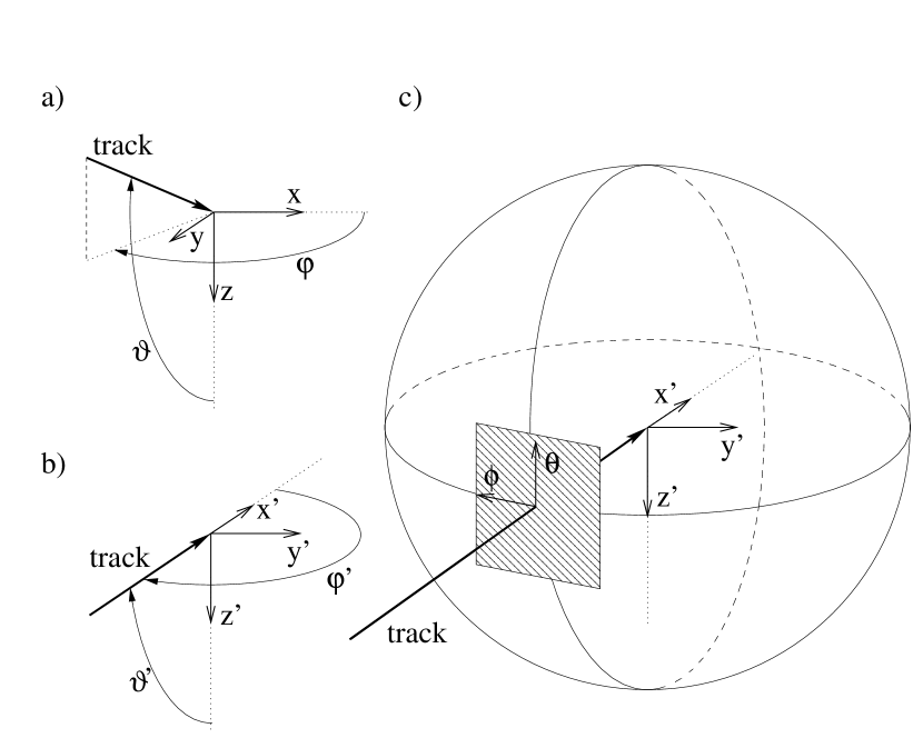
Figure 1: Figure a) shows a track in a Cartesian coordinate system $(x,y,z)$. The direction towards the track’s origin is described with standard spherical coordinates $(\vartheta,\varphi)$. The downward orientation of the $z$-axis follows the AMANDA standards art:recopaper:2004 . In b) a rotated coordinate system $(x^{\prime},y^{\prime},z^{\prime})$ is presented, where the $x^{\prime}$-axis is defined by the track. To describe directions that are close to the track’s direction, relative coordinates $\theta=\vartheta^{\prime}-\pi/2$ and $\phi=\varphi^{\prime}-\pi$ are introduced. They are approximately the coordinates in the tangent plane, as shown in c).

There are two sets of coordinate systems used in the method presented here. The first system uses all five coordinates $(x,y,z,\vartheta,\varphi)$, which are connected to the 3-dimensional Cartesian detector coordinate system as illustrated in Figure 1 a). In the second system the problem is reduced to the 2-dimensional subset of angles $\phi$ and $\theta$.

The complication with $\vartheta$ and $\varphi$ is that the first has boundaries and the second is periodic. Moreover, at the boundaries of $\vartheta$ the variable $\varphi$ becomes meaningless. In a mathematical sense, $\vartheta$ and $\varphi$ are locally orthogonal. However, if one looks at these coordinates in the area surrounding a point, they are distorted - in particular close to $\vartheta=0$ and $\vartheta=\pi$.

As the behaviour of the likelihood function around the well known best track estimate $\mathrm{h}_{\mathrm{best}}$ is to be investigated, the coordinates $\vartheta$ and $\varphi$ should be as close to being orthogonal as possible at that particular direction $(\vartheta_{\mathrm{best}},\varphi_{\mathrm{best}})$. Hence the 3-dimensional detector coordinate system is rotated such that the new x-axis, $x^{\prime}$, is defined by the track. This results in $\vartheta_{\mathrm{best}}^{\prime}=\frac{\pi}{2}$ and $\varphi_{\mathrm{best}}^{\prime}=\pi$, as illustrated in Figure 1 b), where the distortion is minimal.

Here and in the following section 3 only relative coordinates $\theta=\vartheta^{\prime}-\pi$ and $\phi=\varphi^{\prime}-\pi/2$ with respect to $\vartheta_{\mathrm{best}}^{\prime}$ and $\varphi_{\mathrm{best}}^{\prime}$ will be referred to. This can be thought of as local coordinates in the tangential plane to the unit sphere at $(\vartheta_{\mathrm{best}},\varphi_{\mathrm{best}})$ with the origin at the point, where the plane touches the sphere. By choosing a proper rotation, it is assured that the $\theta$-direction is parallel to the $\vartheta$-coordinate, i.e. towards the negative $z/z^{\prime}$-axis. The rotation must be such that the track, the $z$-axis, and the $z^{\prime}$-axis are in the same plane.

The local coordinates are displayed in Figure 1 c).

2.3 Reducing the dimensionality of the problem

The location of the point $\mathbf{r}$ is of no concern for the discussion of where a track points to. Nevertheless the correlations of the errors in direction with the errors in determining $\mathbf{r}$ need to be considered.

The reduction procedure of the dimension shall first be discussed assuming only one spatial dimension $x$ and one directional dimension $\theta$.

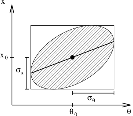
Figure 2: Confidence ellipse in two dimensions with a directional coordinate $\theta$ and a spatial coordinate $x$. The rectangle around the ellipse has the size $2\,\sigma_{\theta}$ by $2\,\sigma_{x}$. Finding for each $\theta$ the corresponding $x$ with extremal likelihood, one arrives at the line shown.

Consider the two-dimensional confidence ellipse in $(\theta,x)$-space (Figure 2). It is tilted versus the $\theta$-axis, which indicates a correlation of $\theta$ and $x$. For each $\theta$ one determines the value of $x$ for which the common likelihood function gets maximal. In the strictly Gaussian case, the result is a straight line. The likelihood function along this line is again a Gaussian as a function of $\theta$. The width of this Gaussian is $\sigma_{\theta}$ as can be seen by straight forward calculation. In this error estimator $\sigma_{\theta}$ the correlation $\mathrm{cov}(\theta,x)$ is included by construction.

The extension to three spatial and two directional dimensions is straight forward: first one determines a set of points in $(\phi_{i},\theta_{i})$. For each point, the best guess, i.e. the best likelihood $l_{i}=-\log\mathcal{L}_{i}$, is found with respect to $\mathbf{r}$.

In the Gaussian approximation these points $l_{i}(\phi_{i},\theta_{i})$ form a paraboloid. Its parameters are found by analytic minimization, which is discussed next.

2.4 The analytic minimization

In order to find the paraboloid that best fits the points $l_{i}(\phi_{i},\theta_{i})$, an analytic $\chi^{2}$-minimization is performed. The paraboloid $f(\phi,\theta;\delta,\beta_{1},\beta_{2},\Gamma)$ is parameterized in its polynomial representation:

$$f(\phi,\theta;\delta,\beta_{1},\beta_{2},\Gamma)=\delta+\beta_{1}\phi+\beta_{2}\theta+\frac{1}{2}(\phi,\theta)\Gamma(\phi,\theta)^{T}\qquad.$$ (2)

The constant parameter is represented by $\delta$ and the parameters in first order by $\beta_{1}$ and $\beta_{2}$. The symmetric $2\times 2$-matrix $\Gamma=\left(\begin{array}[]{cc}\Gamma_{11}&\Gamma_{12}\\ \Gamma_{12}&\Gamma_{22}\end{array}\right)$ contains the second order parameters. Using the method of least squares one calculates

$$\chi^{2}=\sum_{i=1}^{n}(f(\phi_{i},\theta_{i};\delta,\beta_{1},\beta_{2},\Gamma)-l_{i})^{2}=\sum_{i=1}^{n}(\delta+\beta_{1}\phi_{i}+\beta_{2}\theta_{i}+\frac{1}{2}(\phi_{i},\theta_{i})\Gamma(\phi_{i},\theta_{i})^{T}-l_{i})^{2}\qquad,$$ (3)

and requires the minimization conditions

$$\frac{\partial\chi^{2}}{\partial\delta}=\frac{\partial\chi^{2}}{\partial\beta_{i}}=\frac{\partial\chi^{2}}{\partial\Gamma_{ij}}\stackrel{{\scriptstyle!}}{{=}}0\qquad.$$ (4)

This leads to a six-dimensional inhomogeneous system of linear equations:

$$\left(\begin{array}[]{llllll}\sum 1\hphantom{\theta_{i}}&\sum\phi_{i}\hphantom{\theta_{i}}&\sum\hphantom{\theta_{i}}\theta_{i}&\frac{1}{2}\sum\phi_{i}^{2}\hphantom{\theta_{i}}&\sum\phi_{i}\theta_{i}&\frac{1}{2}\sum\hphantom{\theta_{i}}\theta_{i}^{2}\\ \sum\phi_{i}\hphantom{\theta_{i}}&\sum\phi_{i}^{2}\hphantom{\theta_{i}}&\sum\phi_{i}\theta_{i}&\frac{1}{2}\sum\phi_{i}^{3}\hphantom{\theta_{i}}&\sum\phi_{i}^{2}\theta_{i}&\frac{1}{2}\sum\phi_{i}\theta_{i}^{2}\\ \sum\hphantom{\theta_{i}}\theta_{i}&\sum\phi_{i}\theta_{i}&\sum\hphantom{\theta_{i}}\theta_{i}^{2}&\frac{1}{2}\sum\phi_{i}^{2}\theta_{i}&\sum\phi_{i}\theta_{i}^{2}&\frac{1}{2}\sum\hphantom{\theta_{i}}\theta_{i}^{3}\\ \sum\phi_{i}^{2}&\sum\phi_{i}^{3}&\sum\phi_{i}^{2}\theta_{i}&\frac{1}{2}\sum\phi_{i}^{4}&\sum\phi_{i}^{3}\theta_{i}&\frac{1}{2}\sum\phi_{i}^{2}\theta_{i}^{2}\\ \sum\phi_{i}\theta_{i}&\sum\phi_{i}^{2}\theta_{i}&\sum\phi_{i}\theta_{i}^{2}&\frac{1}{2}\sum\phi_{i}^{3}\theta_{i}&\sum\phi_{i}^{2}\theta_{i}^{2}&\frac{1}{2}\sum\phi_{i}\theta_{i}^{3}\\ \sum\hphantom{\theta_{i}}\theta_{i}^{2}&\sum\phi_{i}\theta_{i}^{2}&\sum\hphantom{\theta_{i}}\theta_{i}^{3}&\frac{1}{2}\sum\phi_{i}^{2}\theta_{i}^{2}&\sum\phi_{i}\theta_{i}^{3}&\frac{1}{2}\sum\hphantom{\theta_{i}}\theta_{i}^{4}\\ \end{array}\right)\cdot\left(\begin{array}[]{c}\delta\\ \beta_{1}\\ \beta_{2}\\ (\Gamma)_{11}\\ (\Gamma)_{12}\\ (\Gamma)_{22}\end{array}\right)=\left(\begin{array}[]{l}\sum l_{i}\\ \sum l_{i}\phi_{i}\\ \sum l_{i}\theta_{i}\\ \sum l_{i}\phi_{i}^{2}\\ \sum l_{i}\phi_{i}\theta_{i}\\ \sum l_{i}\theta_{i}^{2}\end{array}\right)$$ (23)

(24)

One can choose the set of points $(\phi_{i},\theta_{i})$ in a suitable way to simplify equation (24). If for each point $(\phi_{i},\theta_{i})$ also $(\phi_{i},-\theta_{i})$, $(-\phi_{i},\theta_{i})$, and $(-\phi_{i},-\theta_{i})$ are added to the set, one arrives at

$$\left(\begin{array}[]{llllll}\sum 1\hphantom{\theta_{i}}&\hphantom{\phi_{i}}0\hphantom{\theta_{i}}&\hphantom{\theta_{i}}0\hphantom{\theta_{i}}&\frac{1}{2}\sum\phi_{i}^{2}\hphantom{\theta_{i}}&\hphantom{\phi_{i}}0\hphantom{\theta_{i}}&\frac{1}{2}\sum\hphantom{\theta_{i}}\theta_{i}^{2}\\ \hphantom{\phi_{i}}0&\sum\phi_{i}^{2}\hphantom{\theta_{i}}&\hphantom{\phi_{i}}0&\hphantom{\phi_{i}}0&\hphantom{\phi_{i}}0&\hphantom{\phi_{i}}0\\ \hphantom{\phi_{i}}0&\hphantom{\phi_{i}}0&\sum\hphantom{\theta_{i}}\theta_{i}^{2}&\hphantom{\phi_{i}}0&\hphantom{\phi_{i}}0&\hphantom{\phi_{i}}0\\ \sum\phi_{i}^{2}&\hphantom{\phi_{i}}0&\hphantom{\phi_{i}}0&\frac{1}{2}\sum\phi_{i}^{4}&\hphantom{\phi_{i}}0&\frac{1}{2}\sum\phi_{i}^{2}\theta_{i}^{2}\\ \hphantom{\phi_{i}}0&\hphantom{\phi_{i}}0&\hphantom{\phi_{i}}0&\hphantom{\phi_{i}}0&\sum\phi_{i}^{2}\theta_{i}^{2}&\hphantom{\phi_{i}}0\\ \sum\hphantom{\theta_{i}}\theta_{i}^{2}&\hphantom{\phi_{i}}0&\hphantom{\phi_{i}}0&\frac{1}{2}\sum\phi_{i}^{2}\theta_{i}^{2}&\hphantom{\phi_{i}}0&\frac{1}{2}\sum\hphantom{\theta_{i}}\theta_{i}^{4}\\ \end{array}\right)\cdot\left(\begin{array}[]{c}\delta\\ \beta_{1}\\ \beta_{2}\\ (\Gamma)_{11}\\ (\Gamma)_{12}\\ (\Gamma)_{22}\end{array}\right)=\left(\begin{array}[]{l}\sum l_{i}\\ \sum l_{i}\phi_{i}\\ \sum l_{i}\theta_{i}\\ \sum l_{i}\phi_{i}^{2}\\ \sum l_{i}\phi_{i}\theta_{i}\\ \sum l_{i}\theta_{i}^{2}\end{array}\right).$$ (43)

(44)

This leads to three equations:

$$\sum\phi_{i}^{2}\cdot\beta_{1} = \sum l_{i}\phi_{i}$$ (45)

$$\sum\theta_{i}^{2}\cdot\beta_{2} = \sum l_{i}\theta_{i}$$ (46)

$$\sum\phi_{i}^{2}\theta_{i}^{2}\cdot(\Gamma)_{12} = \sum l_{i}\phi_{i}\theta_{i}$$ (47)

and a three-dimensional system

$$\left(\begin{array}[]{llllll}\sum 1\hphantom{\theta_{i}}&\frac{1}{2}\sum\phi_{i}^{2}\hphantom{\theta_{i}}&\frac{1}{2}\sum\hphantom{\theta_{i}}\theta_{i}^{2}\\ \sum\phi_{i}^{2}&\frac{1}{2}\sum\phi_{i}^{4}&\frac{1}{2}\sum\phi_{i}^{2}\theta_{i}^{2}\\ \sum\hphantom{\theta_{i}}\theta_{i}^{2}&\frac{1}{2}\sum\phi_{i}^{2}\theta_{i}^{2}&\frac{1}{2}\sum\hphantom{\theta_{i}}\theta_{i}^{4}\\ \end{array}\right)\cdot\left(\begin{array}[]{c}\delta\\ (\Gamma)_{11}\\ (\Gamma)_{22}\end{array}\right) = \left(\begin{array}[]{c}\sum l_{i}\\ \sum l_{i}\phi_{i}^{2}\\ \sum l_{i}\theta_{i}^{2}\end{array}\right)\qquad,$$ (57)

which can easily be solved.

The error estimators sought are contained in the parameters of the paraboloid. The three degrees of freedom of $\delta$ and $\beta_{1,2}$ correspond to the position of the minimum of the curve. The three parameters in $\Gamma$ contain the curvature of the paraboloid, which are functions of the resolution, as the covariance matrix $C$ of the Gaussian approximation is the inverse of $\Gamma$. From $C=\Gamma^{-1}$ one obtains:

$$\sigma_{\phi}^{2} = (\Gamma^{-1})_{11}$$ (58)

$$\sigma_{\theta}^{2} = (\Gamma^{-1})_{22}$$ (59)

$$\mathrm{cov}(\phi,\theta) = (\Gamma^{-1})_{12}\qquad.$$ (60)

Figure 3: The confidence ellipse in $\theta$ and $\phi$ can be represented either by $\sigma_{\theta}$, $\sigma_{\phi}$, and the covariance $\mathrm{cov}(\theta,\phi)$ or by the major and minor axes $\sigma_{1}$ and $\sigma_{2}$, and the rotation angle $\alpha$ of the ellipse between the major axis and the $\theta$-direction.

The results can also be represented in a more intuitive way using the major and the minor axes $\sigma_{1}$ and $\sigma_{2}$ of the confidence ellipse, and its rotation angle $\alpha$ with respect to the $\phi$-axis (Figure 3). In order to find this alternative representation, the covariance matrix $C$ needs to be diagonalized. That leads to

$$\sigma_{1,2}^{2}=\frac{\sigma_{\phi}^{2}+\sigma_{\theta}^{2}}{2}\pm\sqrt{\frac{(\sigma_{\phi}^{2}+\sigma_{\theta}^{2})^{2}}{4}+\det C}\qquad.$$ (61)

Choosing $\sigma_{1}\geq\sigma_{2}$, the rotation angle $\alpha$ is then given by the expression

$$\tan\alpha=\frac{\sigma_{1}^{2}-\sigma_{\phi}^{2}}{\mathrm{cov}(\phi,\theta)}\qquad.$$ (62)

In the following discussion a third representation $(\sigma_{\mathrm{a}},\epsilon,\alpha)$ will be used, where $\sigma_{\mathrm{a}}$ is connected to the area of the ellipse and $\epsilon$ is its excentricity:

$$\sigma_{\mathrm{a}} = \sqrt{\sigma_{1}\cdot\sigma_{2}}$$ (63)

$$\epsilon = \frac{\sigma_{1}}{\sigma_{2}}\qquad.$$ (64)

The rotation angle $\alpha$ is the same as in the previous parameterization.

This procedure can lead to unphysical, negative values for the variance estimators. This happens whenever the basic track finding procedure has not arrived at a good minimum in likelihood space. The search for the minimum should then be repeated more carefully.

Note, that the resolution estimates are calculated for each pattern of hits seperately. Still they are not the true values for the discrepancies of true and reconstructed direction, but estimates of the average discrepancy for a set of events, which are similar to the one under consideration.

3 Space angle resolution

For a neutrino telescope it is common to quote the median $\bar{\Psi}$ of the spatial angle $\Psi$ between true and reconstructed track direction in order to describe its resolution. This section is devoted to the connection of the error ellipse parameters to the space angle uncertainty $\psi$. It is convenient to choose the representation of the ellipse using $\sigma_{\mathrm{a}}$ and $\epsilon$, with $\alpha$ not playing a role in this special context.

The true direction lies within the area given by the error ellipse with a probability of $39.4\%$. The median of a distribution corresponds to a $50\%$-probability. Hence as a first step the ellipses need to be enlarged correspondingly.

In order to obtain $\psi$, one considers the Gaussian likelihood function in its diagonal form, where the coordinates are $x_{1}$ and $x_{2}$:

$$f(x_{1},x_{2})=\frac{1}{2\pi\sigma_{1}\sigma_{2}}e^{-\frac{1}{2}\left(\left(\frac{x_{1}}{\sigma_{1}}\right)^{2}+\left(\frac{x_{2}}{\sigma_{2}}\right)^{2}\right)}\qquad.$$ (65)

To obtain the median $\mathrm{M}$, the function $f(x_{1},x_{2})$ must be integrated from the center $(0,0)$ outwards until a cumulated probability of $0.5$ is reached. This integral is done in polar coordinates (radius $\rho$ and angle $\gamma$)

$$0.5\stackrel{{\scriptstyle!}}{{=}}\int_{0}^{\mathrm{M}}\int_{0}^{2\pi}f\left(\rho\cos\gamma,\rho\sin\gamma\right)\rho\,\mathrm{d}\gamma\,\mathrm{d}\rho\qquad.$$ (66)

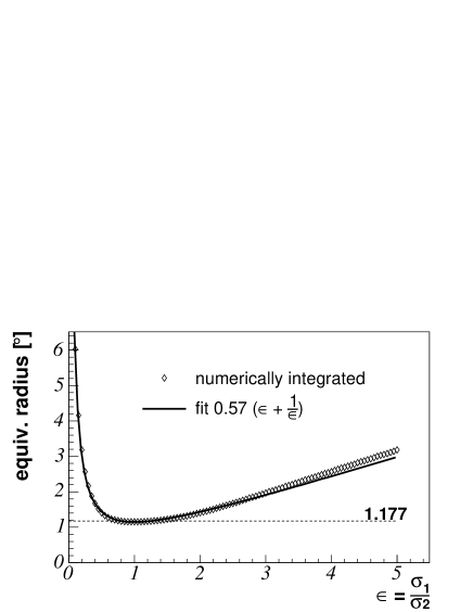
For the special case of $\sigma_{\mathrm{a}}=\sigma_{1}=\sigma_{2}$ (i.e. $\epsilon=1$), the calculation can be carried out analytically and yields $\mathrm{M}=1.177\cdot\sigma_{\mathrm{a}}$.

Figure 4: Obtaining the space angle resolution estimate by applying a correction based on the excentricity. For fixed $\sigma_{\mathrm{a}}=1^{\circ}$ and varying $\epsilon$, the equivalent radius $\mathrm{M}$ is displayed, such that the true direction lies within a circle of radius $\mathrm{M}$ with a probability of $50\%$.

For the general case (with arbitrary $\epsilon$) the integration must be carried out numerically. This has been done for the case of $\sigma_{\mathrm{a}}=1^{\circ}$ and the result is shown in Figure 4. The median $\mathrm{M}$ scales linearly with $\sigma_{\mathrm{a}}$.

The curve is symmetric with respect to the exchange of $\sigma_{1}$ and $\sigma_{2}$. To improve the speed of the program an approximation proportional to $(\epsilon+\frac{1}{\epsilon})$ has been applied which results in the excentricity corrected spatial angle resolution estimation:

$$\sigma_{a}^{\epsilon}=0.57\cdot(\epsilon+\frac{1}{\epsilon})\cdot\sigma_{a}\qquad.$$ (67)

The fit is also shown in Figure 4. The deviation in the interval $\epsilon\in[1;3]$ is below $5\%$. For applications where this is too coarse an approximation, the exact results of the numerical integration can be stored in appropriate tables.

4 Discussion

The above algorithms have been tested within the framework of the AMANDA neutrino telescope. The estimates perform in a stable and reliable way and produce sensible results.

To ensure the correctness of the estimations, several testing procedures both in data and in Monte Carlo have been carried out:

1. For $\sigma_{\theta}$ and $\sigma_{\phi}$ its pull has been studied. It is defined as the ratio of the difference of true and reconstructed direction over the resolution estimator. If the estimation is good, the pull should be Gaussian distributed, centered at zero and with unit width. This investigation can only be done in a Monte Carlo simulation.

2. For the spatial angle resolution the pull is not a sensible quantity, because angles in space can only be positive. Hence one can study ensembles of events with the same $\sigma_{\mathrm{a}}$ or $\sigma_{\mathrm{a}}^{\epsilon}$, respectively. The median of the true deviation can then be compared to the corresponding $\sigma_{\mathrm{a}}$. Again this can only be done in the simulation.

3. In data the true directions are not known. Thus another approach is being followed. Each event is split into two subevents by assigning every second hit to subevent 1 and the remaining hits to subevent 2. Each subevent undergoes reconstruction and is subjected to the resolution estimation algorithm. That leads to directions $\vartheta^{i}$, $\varphi^{i}$ and errors $\sigma_{\theta}^{i}$ und $\sigma_{\phi}^{i}$ with $i\in\{1,2\}$.

   The pull

   $$\mathrm{P}_{\vartheta}=\frac{\mathrm{D}_{\vartheta}}{\sigma_{\theta}^{\mathrm{D}}}=\frac{\vartheta^{1}-\vartheta^{2}}{\sqrt{(\sigma_{\theta}^{1})^{2}+(\sigma_{\theta}^{2})^{2}}}$$ (68)

   should also be a Gaussian distribution centered at zero with unit width. For $\mathrm{P}_{\varphi}$ the difference in azimuth angles must be multiplied by $\sin\vartheta$ to make up for the differences in the rotated and not rotated coordinate systems:

   $$\mathrm{P}_{\varphi}=\frac{\mathrm{D}_{\varphi}}{\sigma_{\phi}^{\mathrm{D}}}=\frac{(\varphi^{1}-\varphi^{2})\cdot\sin\vartheta}{\sqrt{(\sigma_{\phi}^{1})^{2}+(\sigma_{\phi}^{2})^{2}}}\qquad.$$ (69)

   Of course this last check can also be done in the simulation.

In all tests the results were satisfactory. Further details about the tests and their results can be found in phd:neunhoeffer_eng:2003 .

4.1 Concluding remarks

1. Often one applies quality cuts to the data set, which rely on additional information that is not reflected in the construction of the likelihood function itself. Hence this information is also not used in obtaining the resolution parameters. In this case one expects the selected tracks to be on average closer to the true direction than from the likelihood analysis alone. Consequently one observes a pull with a width smaller than 1.

2. The resolution parameters - such as $\sigma_{\mathrm{a}}$ - can efficiently be used as cut variables, as misreconstructed events on average have a worse resolution than correctly reconstructed ones.

3. The resolution estimation on an event-per-event basis can be used as additional input in point source searches. The information is hard to be included in the commonly used binned search algorithms tillpub:ahrens:2003xy3 . An appropriate procedure based on maximum likelihood methods that can integrate the new information in a natural way will be presented in a forthcoming publication.

References

• [1] J.Β Ahrens etΒ al. Muon track reconstruction in AMANDA. Nucl. Instrum. Methods, 2004. in press.
• [2] J.Β Ahrens etΒ al. Search for extraterrestrial point sources of neutrinos with AMANDA-II. Phys. Rev. Lett., 92:071102, 2004, astro-ph/0309585.
• [3] E.Β Andres etΒ al. Observation of high-energy neutrinos using Cerenkov detectors embedded deep in Antarctic ice. Nature, 410:441–443, 2001.
• [4] Till NeunhΓΆffer. Development of a new method to search for cosmic neutrino point sources with the AMANDA neutrino telescope. Ph.D. thesis, University of Mainz, Germany, 2004. (Shaker Verlag, Aachen, ISBN 3-8322-2474-2, in German).