An X-ray measurement of Titan’s atmospheric extent from its transit of the Crab Nebula
Abstract
Saturn’s largest satellite, Titan, transited the Crab Nebula on 5 January 2003. We observed this astronomical event with the Chandra X-ray Observatory. An “occultation shadow” has clearly been detected and is found to be larger than the diameter of Titan’s solid surface. The difference gives a thickness for Titan’s atmosphere of 880 60 km. This is the first measurement of Titan’s atmospheric extent at X-ray wavelengths. The value measured is consistent with or slightly larger than those estimated from earlier Voyager observations at other wavelengths. We discuss the possibility of temporal variations in the thickness of Titan’s atmosphere.
1 INTRODUCTION
Titan is the only satellite in the solar system with a thick atmosphere. Its atmosphere has a pressure near the surface is about 1.5 times greater than that of the Earth at sea level and extends much further than that of the Earth (Coustenis & Lorenz 1999). Titan’s atmosphere is known to resemble the primitive environment of the Earth’s atmosphere in terms of chemistry, providing us with a laboratory to study the origin of life (Owen et al. 1997). The atmospheric structure of Titan has been investigated at radio (Lindal et al. 1983), infrared (IR) (Lellouch et al. 1989), optical (Sicardy et al. 1990; Hubbard et al. 1990), and ultraviolet (UV) wavelengths (Strobel, Summers, & Zhu 1992; Smith et al. 1982). These results came from the Voyager 1 spacecraft during its encounter with Titan and from a stellar occultation by Titan. Due to the wavelength dependence of transmissivity, the radio, IR, and optical observations measure the thermal structure of Titan’s atmosphere below an altitude of 500 km while the UV observation measures it above an altitude of 1000 km. No direct information has hitherto been obtained at intermediate altitudes where the X-ray observation is effective.
On 5 January 2003, the Saturnian system passed across the wide X-ray bright region of the Crab Nebula. The Saturnian system has a conjunction with the Crab Nebula every 30 years. However, because of an average offset of a few degrees, it rarely transits the Crab Nebula. Although a similar conjunction occurred once in January of 1296, the Crab Nebula, which is a remnant of SN1054, must have been too small to be occulted. Therefore, this may be the first transit since the birth of the Crab Nebula. The next similar conjunction will take place in August of 2267, making its occurrence in 2003 a “once-in-a-lifetime” event. The Saturnian system is a million times brighter in visible light than the Crab Nebula whereas the Crab Nebula is a million times brighter in X-rays than the Saturnian system. This prevented us from observing the transit in the optical, but provided a unique opportunity for an X-ray observation which had never been performed. The Crab Nebula is one of the brightest synchrotron sources in the sky and, thus, makes an ideal diffuse background light source to study X-ray shadows of interesting objects.
Here, we report results from an observation of this historical event with the Advanced CCD Imaging Spectrometer (ACIS) aboard the Chandra X-ray Observatory. Chandra has an angular resolution of and can resolve Saturn, its rings, and the satellite Titan, whose angular size is about . Unfortunately, it was not possible to observe the transit of Saturn due to Chandra’s concurrent passage through the Earth’s radiation zone. Only Titan was observable because Chandra had passed through the radiation zone by the time Titan transited 12 hours later. We describe the observation in §2. The data analysis and results are presented in §3. Comparison with previous observations and implications of this observation will be discussed in §4.
2 OBSERVATION
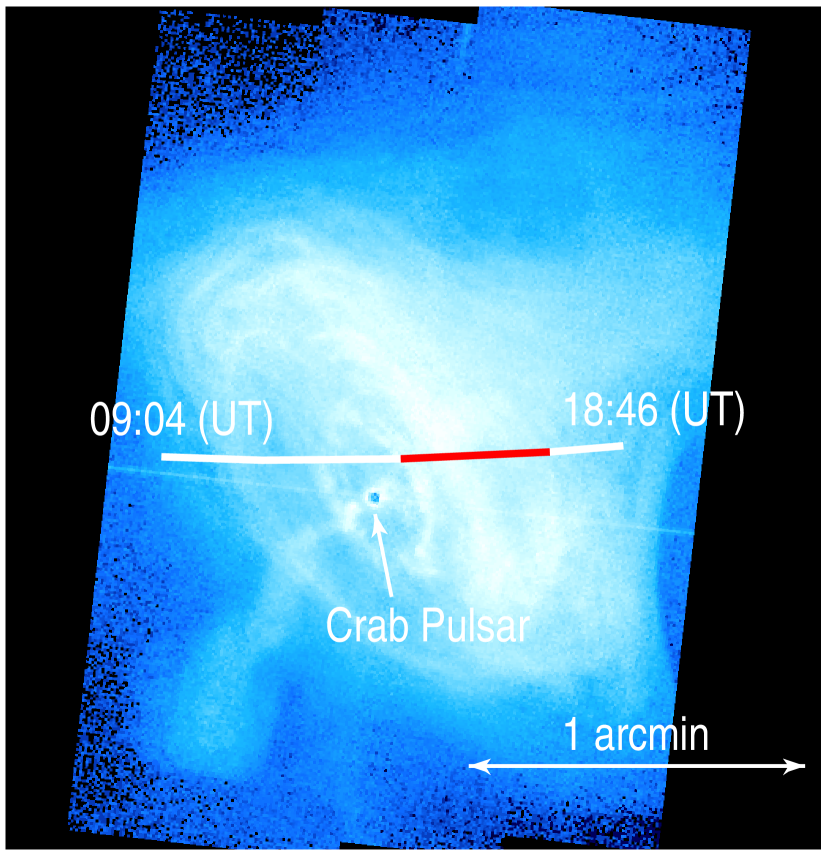
The observation was performed from 09:04 to 18:46 (UT) on 5 January 2003. Figure 1 shows the Titan transit path on the Crab Nebula. In order to avoid event pile-up and telemetry saturation, which made difficulties for analysis of previous Chandra observations of the Crab Nebula (Weisskopf et al. 2000; Hester et al. 2002), we inserted a transmission grating, shortened the CCD frame time from the nominal value of 3.2 seconds to 0.3 seconds, and adopted a small subarray window (). These observational modes did work efficiently to result in no telemetry saturation and no apparent event pile-up. We will carefully investigate the possibility of the event pile-up effect on our result in §3.2.3. Since the restricted window could not cover the whole Titan transit path, we changed the pointing direction twice during the observation. In spite of the time loss due to the two maneuvers, we obtained an effective exposure time of 32279 seconds, which corresponds to 92% of the total observing time duration.
3 ANALYSIS AND RESULTS
3.1 Reprojection To the Titan Fixed Frame
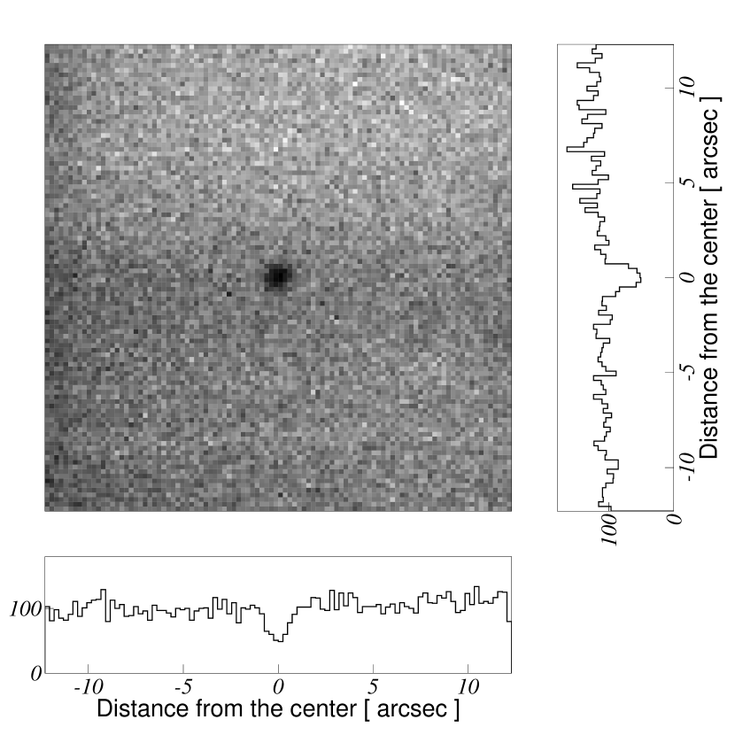
No hint of the Titan transit can be seen in the standard sky image in Figure 1. Titan moved too fast to cast an observable shadow against the Crab Nebula in the sky image. In order to search for a shadow, we reprojected each photon’s position to a frame fixed with respect to Titan. We used CIAO111Chandra Interactive Analysis of Observations. See http://cxc.harvard.edu/ciao/ tool sso_freeze for the reprojection. Before applying sso_freeze, we removed the pixel randomization, which was applied by default in the standard data processing, and applied our subpixel resolution method (Tsunemi et al. 2001; Mori et al. 2001)222See http://asc.harvard.edu/cont-soft/software/subpixel_resolution.1.4.html to obtain the best available spatial resolution. Figure 2 shows the Titan fixed frame image. A clear shadow can be seen, which was made by Titan’s occultation of the Crab Nebula. Measurement of the effective radius of the occultation shadow provides us with information on Titan’s atmospheric extent.
3.2 Effective Radius of the Occultation Shadow
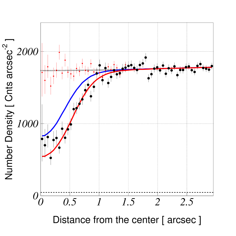
Figure 3 shows a radial profile of the photon number density from the center of the occultation shadow (black points). From this radial profile, we computed the effective radius of the occultation shadow, .
3.2.1 Method
We assumed that the distribution of photons in Figure 2 is symmetric with respect to the center of the occultation shadow. The observed photon number density as a function of the distance from the center of the occultation shadow, , can be given by a convolution of the intrinsic photon number density, , and the point spread function (PSF), :
| (1) |
The Chandra PSF has a very sharply peaked core with extended wings and is strongly energy dependent due to larger scattering of higher energy photon by the mirror surface (Chandra Proposers’ Observatory Guide 2002). In general, it is quite difficult to obtain a precise analytical form of the PSF, which prevents us from solving equation 1 to obtain directly from . Instead, its numerical form can be generated through a raytrace code which has been determined by the Chandra team on the basis of both ground-based and on-orbit calibrations. Therefore, we performed Monte Carlo simulations incorporating the numerical form of the PSF. We approximated by a step function with a threshold radius, . We fitted the data points in Figure 3 with , varying to obtain the best fit. is defined by which gives the minimum . Justification for the approximation using the step function will be discussed in §4.
The PSF was derived from raytrace tools ChaRT333Chandra Ray Tracer. See http://asc.harvard.edu/chart/ and MARX444See http://space.mit.edu/CXC/MARX/. ChaRT provides the best available mirror response at any off-axis angle and for any spectrum. MARX reads the output of ChaRT and creates the PSF taking into account the detector responses and aspect reconstruction uncertainties. We obtained the PSF appropriate for the observation conditions: at off-axis angle of about and for the observed spectrum. The output PSF from MARX includes the pixel randomization. Since the pixel randomization broadens PSF, we sharpened it by the appropriate amount. To account for our application of the subpixel method, we further sharpened the PSF by 5% in terms of the Half Power Diameter (HPD), which is the expected improvement for this off-axis angle on the ACIS-S CCD (Tsunemi et al. 2002; Mori et al. 2002). The HPD of the resultant PSF was . We will discuss the validity of this PSF in §3.2.3.
In order to compare the results of the Monte Carlo simulation with the data, we must also account for gradients in the sky background level and for instrumental effects like trailing events. A big advantage of our observation was the ability to determine the background level across the shadow based on knowledge of the surface brightness of the Crab Nebula along the Titan transit path. We derived the background profile across the shadow by averaging two profiles which were taken centered at ahead of and behind of the occultation shadow center. The background profiles are presented as red points in Figure 3. Then, the gradient of the background was determined by fitting the red points within the shadow () and the black points outside of it with a quadratic function, which is shown with a dotted line in Figure 3.
The trailing events are defined as events detected during the CCD readout. Since the positions of the trailing events are recorded improperly along the readout direction, they cause an offset in the image. The contribution of the trailing events to the total photon number density can be evaluated because its level is proportional to the fraction of the total effective exposure time spent in transferring the charge across the X-ray bright region, . In the case of ACIS, it takes 40 sec to transfer the charge from one pixel to another. The width of the X-ray bright region along the readout direction is about 210 pixels (; see Fig. 1). Therefore, it takes 0.0084 seconds to transfer the charge across the X-ray bright region. Since CCD frame time is 0.3 seconds, becomes %. The resultant estimate for the background level due to the trailing events is shown as a dashed line in Figure 3.
3.2.2 Result
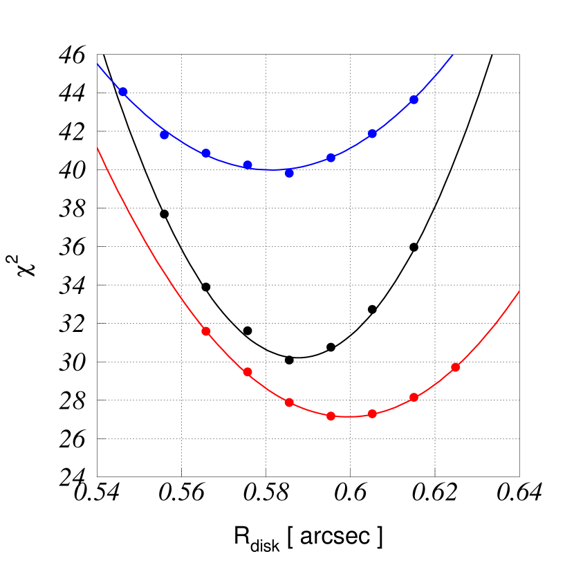
The first 30 data points from the center () were used for the test because data points further from the center hardly affected the result. Figure 4 shows as a function of . The values are well described with a quadratic function. The best fit value was obtained as arcseconds with / d.o.f of 30.36 / 29. The uncertainty is 68.3% (1) confidence level. The best fit curve is shown in Figure 3 (red line) along with a curve simulating (blue line) which corresponds to the radius of the Titan solid surface (2575 km). The difference between those two curves is attributed to X-ray absorption by Titan’s atmosphere.
3.2.3 Systematic checks
The validity of the PSF, the effect of event pile-up, and the contribution from the intrinsic background of ACIS were examined. The accuracy of the adopted PSF was checked using a point source in the Orion Nebula Cluster, CXOONC J053514.0-052338, located at a J2000 position of 05h35m1406, 05°23′384 (Getman et al. in preparation). The point source has an off-axis angle of , comparable with that of Titan in our observation. We processed the data of the point source in the same manner described in §3.2.1; removing the pixel randomization and applying the subpixel resolution method. The PSF was obtained again through ChaRT/MARX, but appropriate for the spectrum of the point source, and was sharpened again in the same manner described in §3.2.1. We confirmed that the PSF originally obtained from ChaRT/MARX had a HPD 15% larger than that of the point source, but that the PSF sharpened for our data processing effects was consistent with the point source data to within a few percent. Next, we studied the dependency of on the PSF by performing simulations using PSFs with 10% larger and smaller HPDs than that of adopted one. In an ideal case, even if a wrong PSF was used, would be always the same although the value would increase and the fit would not be statistically acceptable. In reality, depended on the HPD; became larger and smaller by about 0.018 arcseconds which is comparable to about a 1.6 statistical error. However, considering that the adopted PSF is accurate to a few percent, we can safely assume that this dependency is negligible compared with the statistical error. We note that those simulations using broader and narrower PSFs resulted in higher value by about 3 than the simulation described in §3.2.1, also supporting the validity of the adopted PSF. Therefore, we conclude that the adopted PSF is reliable and its uncertainty hardly affected the result.
In order to examine the pile-up effect, the data were divided into two time intervals according to flux level, “high flux time interval” and “low flux time interval”. The division is indicated in Figure 1. The average background count rates in the high and low flux time intervals are 8.1 and 4.0 counts sec-1 arcsec-2, respectively. Separate calculations of for the two data sets were performed in the same way described above. Plots of as a function of are shown in Figure 4. The resultant values were and arcseconds for the high and low flux time intervals, respectively. Since the values are statistically consistent with each other and with the result obtained using all the data, we conclude that event pile-up is unlikely to have affected the result.
The contribution of the intrinsic ACIS background cannot be a problem because it is about 1.5 10-6 counts sec-1 arcsec-2 (Chandra Proposers’ Observatory Guide 2002). It is three order of magnitude lower than that of the trailing events.
4 DISCUSSION
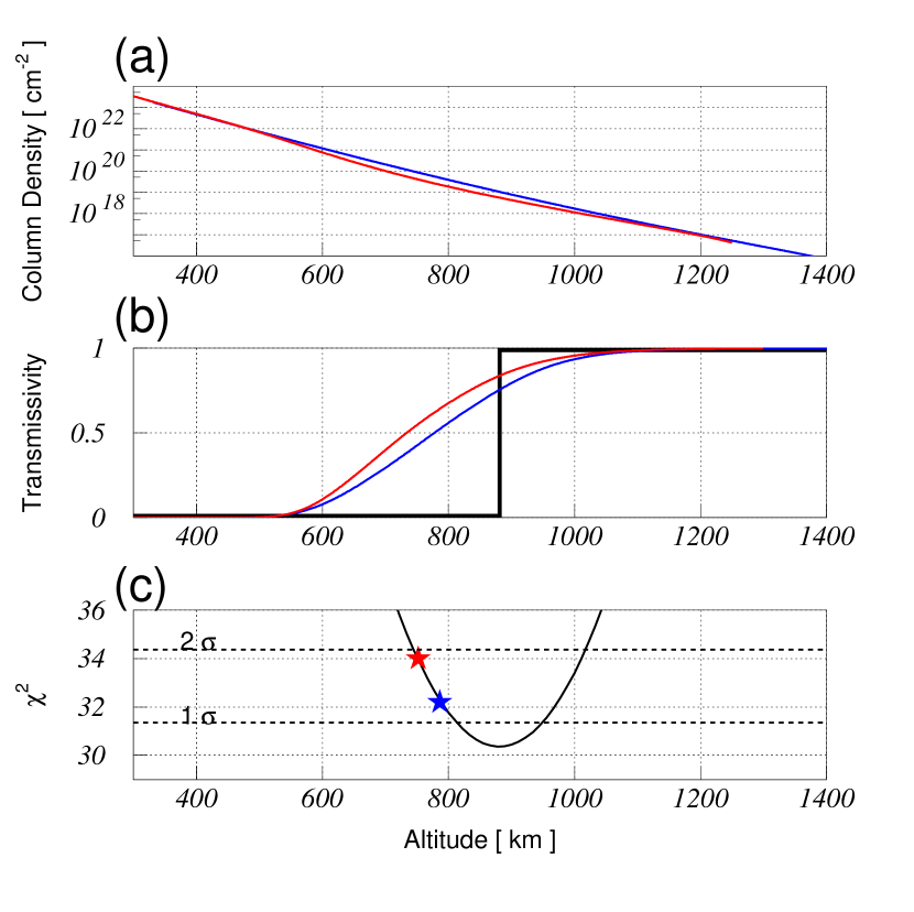
Taken with the distance of 1.214 109 km to Titan at the time of this observation, arcseconds gives a thickness for Titan’s atmosphere of km. This value can be compared with estimates from the models for Titan’s atmosphere which have been constructed based on Voyager 1 observations at radio, IR, and UV wavelengths. Figure 5a shows profiles of the tangential column density (cm-2) along the line-of-sight as a function of altitude (distance above Titan’s surface), which are compiled from density (cm-3) profiles provided by Yelle et al. (1997) (red) and Vervack, Sandel, & Strobel (manuscript in preparation) (blue). Nitrogen dominates, making up more than 95% of the atmospheric constituents, and methane is the second major component, although proportions slightly differ in the two models. In those models, the profiles in the altitude range of 500–1000 km, where no data were available, were interpolated between the data of higher and lower altitudes assuming hydrostatic equilibrium. The step function we used to determine the atmospheric thickness is a simplification of the transmission curve of X-rays through the atmosphere. In reality, X-rays suffer photoelectric absorption as they pass through the atmosphere, with a transmissivity determined by the atmospheric composition, the tangential column density for a given altitude, and photon energy. We have calculated transmission curves by using the atmospheric compositions of the above two models, the tangential column densities in Figure 5a, and integrating over the observed Crab spectrum. The curves are shown in Figure 5b. The step function with a threshold of is also shown. Figure 5c shows a curve which is identical with the black curve shown in Figure 4, but the definitions of the x-axis are different. We compared the simulation treating the atmosphere as a solid disk (disk model) with the simulations based on the transmission curves shown in Figure 5b (atmosphere model) as follows. We calculated for the atmosphere model simulations and defined the “characteristic altitude” for those models by
| (2) |
where is transmissivity as a function of altitude, . We find that = 750 and 780 km for the Yelle et al. and Vervack et al. models, respectively. The points (, ) for those two atmosphere models fall very close to the curve for the disk model, as shown in Figure 5c. In other words, our step-function transmissivity is indistinguishable from a more realistic transmissivity with at the threshold of the step in the simulation. This fact strongly justifies the approximation of transmission curve with a step function in our simulation and suggests that and can be directly compared with each other. Then, our result for the thickness of Titan’s atmosphere is consistent with or slightly larger than those estimated from Voyager 1 observations (1.9 and 1.4 separation).
Although the statistical significance is not so large, it is still worth discussing a temporal variation of Titan’s upper atmosphere. Distances between the Sun and Saturn were 1.42 and 1.35 109 km at the time of Voyager’s encounter (November 1980) and our observation (January 2003), respectively. The solar luminosity is known to be fairly stable with an uncertainty of 0.3% regardless of its 11 years active cycle (Fröehlich & Lean 1998; Quinn & Fröehlich 1999). Accordingly, the closer distance to the Sun in our observation might have resulted in the higher temperature and the larger extent of the atmosphere. Although the size of this effect cannot be ascertained without detailed modeling, the increase in solar flux incident on Titan may account for some part of the slightly larger value of Titan’s atmosphere measured here. More detailed information will be obtained by the Cassini/Huygens mission in 2005.
Finally, we note that the spectrum taken from the shadow has no absorption nor emission line feature and is statistically indistinguishable from the spectrum taken from the surrounding region. Those facts indicate that photons penetrating the atmosphere hardly contributed to the spectrum taken from the shadow; if they did, excess absorption due to Titan’s atmosphere would be seen in the shadow spectrum. The absence of excess absorption is reasonable considering that the PSF is much broader (the HPD corresponds to about 5000 km) than the corresponding atmospheric thickness interval of about 500 km within which the tangential optical depth changes from unity to zero (see Fig. 5b).
References
- Coustenis & Lorenz (1999) Coustenis A., & Lorenz, R. D. 1999, in Encyclopedia of the Solar System, P. Weissman, L. McFadden, T. Johnson, Eds. (London, Academic Press) pp. 377-404
- Chandra Proposers’ Observatory Guide (2002) Chandra Proposers’ Observatory Guide, Version 5.0, 2002, http://asc.harvard.edu/proposer/POG/index.html
- Fröehlich & Lean (1998) Fröehlich, C., & Lean, J. 1998, Geophys. Res. Let. 25, 4377
- Hester et al. (2002) Hester, J. J., Mori, K., Burrows, D. N. et al. 2002, ApJ, 577, L49
- Hubbard et al. (1990) Hubbard, W. B., Hunten, D. M., Reitsema, H. J., Brosch, N., Nevo, Y., Carreira, E., Rossi, F., & Wasserman, L. H. 1990, Nature, 343, 353
- Lellouch et al. (1989) Lellouch, E., Coustenis, A., Gautier, D., Raulin, F., Dubouloz, N. & Frere, C. 1989, Icarus, 79, 328
- Lindal et al. (1989) Lindal, G. F., Wood, G. E., Hotz, H. B., Sweetnam, D. N., Eshleman, V. R., & Tyler, G. L. 1983, Icarus, 53, 348
- Mori et al. (2001) Mori, K., Tsunemi, H., Miyata, E., Baluta, C., Burrows, D. N., Garmire, G. P., & Chartas, G. 2001, in ASP Conf. Ser. 251, New Century of X-Ray Astronomy, ed. H. Inoue & H. Kunieda (San Francisco: ASP), 576
- Owen et al. (1997) Owen, T., Raulin, F., McKay, C. P., Lunine, J. I., Lebreton, J. -P., & Matson, D. L. 1997, in Huygens, Payload and Mission, ESA SP-1177
- (10) Quinn, T. J., & Fröehlich, C. 1999, Nature 401, 841
- Sicardy et al. (1990) Sicardy, B. et al. 1990, Nature, 343, 350
- Smith et al. (1982) Smith, G. R., Strobel, D. F., Broadfoot, A. L., Sandel, B. R., Shemansky, D. E., & Holberg, J. B. 1982, J. Goephys. Res., 87, 1351
- Strobel et al. (1992) Strobel, D. F., Summers, M. E., & Zhu, X. 1992, Icarus, 100, 512
- tsunemi et al. (2001) Tsunemi, H., Mori, K., Miyata, E., Baluta, C., Burrows, D. N., Garmire, G. P., & Chartas, G. 2001, ApJ, 554, 496
- Weisskopf et al. (2000) Weisskopf, M. C., Hester, J. J., Tennant, A. F., et al. 2000, ApJ, 536, L81
- Yelle et al. (1997) Yelle, R. V., Strobel, D. F., Lellouch, E., & Gautier, D. 1997, Eur. Space Agency Sci. Tech. Rep., ESA SP-1177, 243
