A Hybrid Cosmological Hydrodynamic/N-body Code Based on a Weighted Essentially Non-Oscillatory Scheme

Abstract

We present a newly developed cosmological hydrodynamics code based on weighted essentially non-oscillatory (WENO) schemes for hyperbolic conservation laws. WENO is a higher order accurate finite difference scheme designed for problems with piecewise smooth solutions containing discontinuities, and has been successfully applied for problems involving both shocks and complicated smooth solution structures. We couple hydrodynamics based on the WENO scheme with standard Poisson solver - particle-mesh (PM) algorithm for evolving the self-gravitating system. The third order low storage total variation diminishing (TVD) Runge-Kutta scheme has been used for the time integration of the system. To test accuracy and convergence rate of the code, we subject it to a number of typical tests including the Sod shock tube in multidimensions, the Sedov blast wave and formation of the Zeldovich pancake. These tests validate the WENO hydrodynamics with fast convergence rate and high accuracy. We also evolve a low density flat cosmological model ($\Lambda$CDM) to explore the validity of the code in practical simulations.

1 Introduction

Though the universe seems to be dominated by the dark sides of both matter and energy (Turner, 2002), the observed luminous universe has been existing in the form of baryonic matter, whose mass density, constrained by the primordial nucleosynthesis (Walker, et al., 1991), only occupies a small amount of the total density. To account for the observational features revealed by the baryonic matter, i.e., X-ray emitting gas in galaxies and clusters (Mulchaey, 2000), intergalactic medium inferred from Ly$\alpha$ forest (Rauch, 1998), X-ray background radiation (Giacconi et al. 1962) and distorted spectrum of the cosmic background radiation due to the Sunyaev-Zeldovich effect (Zel’dovich & Sunyaev 1969; Ostriker & Vishniac 1986) etc., it would be necessary to incorporate hydrodynamics into cosmological investigations. This motivation has stimulated great efforts to apply a variety of gas dynamics algorithms to cosmological simulations. For a general review of the state-of-the-art on this topic, we refer to Bertschinger (1998).

Due to the high non-linearity of gravitational clustering in the universe, there are two significant features emerging in cosmological hydrodynamic flow, which pose more challenges than the typical hydrodynamic simulation without self-gravity. One significant feature is the extremely supersonic motion around the density peaks developed by gravitational instability, which leads to strong shock discontinuities within complex smooth structures. Another feature is the appearance of an enormous dynamic range in space and time as well as in the related gas quantities. For instance, the hierarchical structures in the galaxy distribution span a wide range of length scales from a few kpc resolved by individual galaxy to several tens of Mpc characterizing the largest coherent scale in the universe.

A variety of numerical schemes for solving the coupled system of collisional baryonic matter and collisionless dark matter have been developed in the past decades. They fall into two categories, particle methods and grid based methods.

The particle methods include variants of the smooth-particle hydrodynamics (SPH; Gingold & Monagham 1977, Lucy 1977) such as those of Evrard (1988), Hernquist & Katz (1989), Navarro & White (1993), Couchman, Thomas & Pierce (Hydra, 1995), Steinmetz (1996), Owen et al. (1998) and Springel, Yoshida & White (Gadget, 2001). The SPH method solves the Lagrangian form of the Euler equations, and could achieve good spatial resolutions in high density regions, but works poorly in low density regions. It also suffers from degraded resolution in shocked regions due to the introduction of sizable artificial viscosity.

The grid based methods are to solve the Euler equations on structured or unstructured grids. The early attempt was made by Cen (1992) using a central difference scheme. It uses artificial viscosity to handle shocks and has first-order accuracy. The modern approaches implemented for high resolution shock capturing are usually based on the Godunov algorithm. The two typical examples are the total-variation diminishing (TVD) scheme (Harten 1983) and the piecewise parabolic method (PPM) (Collella & Woodward 1984). Both schemes start from the integral form of conservation laws of Euler equations and compute the flux vector based on cell averages (finite volume scheme). The TVD scheme modifies the flux using an approximate solution of the Riemann problem with corrections added to ensure that there are no postshock oscillations. While in the PPM scheme, the Riemann problem is solved accurately using a quadratic interpolation of the cell-average densities that is constrained to minimize postshock oscillations. In the cosmological setting, the TVD based codes include those of Ryu et al. (1993), the moving-mesh scheme (Pen, 1998), and the smooth Lagrangian method (Gnedin, 1995); and the PPM based codes include those of Stone & Norman (Zeus; 1992), Bryan et al. (1995), Sornborger et al. (1996), Ricker, Dodelson & Lamb (COSMOS; 2000). The grid-based methods suffer from the limited spatial resolution, but they work extremely well both in low and high density regions as well as in shocks. To reach a large dynamical range, the Godunov methods have also been implemented with adaptive mesh refinement (RAMSES: Teyssier, 2002; ENZO: Norman & Bryan, 1999; O’Shea et al., 2004), which is more adequate to explore the fine structures in the hydrodynamic simulation.

We describe in this paper an alternative hydrodynamic solver which discretizes the convection terms in the Euler equations by the fifth order finite difference WENO (weighted essentially non-oscillatory) method, first developed in Jiang & Shu (1996), with a low storage third order Runge-Kutta time discretization, which was proven to be nonlinearly stable in Gottlieb & Shu (1998). The WENO schemes are based on the essentially non-oscillatory (ENO) schemes first developed by Harten et al. (1987) in the form of finite volume scheme for hyperbolic conservative laws. The ENO scheme generalizes the total variation diminishing (TVD) scheme of Harten (1983). The TVD schemes typically degenerate to first-order accuracy at locations with smooth extrema while the ENO scheme maintains high order accuracy there even in multi-dimensions. WENO schemes further improve upon ENO schemes in robustness and accuracy. Both ENO and WENO schemes use the idea of adaptive stencils in the reconstruction procedure based on the local smoothness of the numerical solution to automatically achieve high order accuracy and non-oscillatory property near discontinuities. For WENO schemes, this is achieved by using a convex combination of a few candidate stencils, each being assigned a nonlinear weight which depends on the local smoothness of the numerical solution based on that stencil. WENO schemes can simultaneously provide a high order resolution for the smooth part of the solution, and a sharp, monotone shock or contact discontinuity transition. WENO schemes are extremely robust and stable for solutions containing strong shocks and complex solution structures. Moreover, a significant advantage of WENO is its ability to have high accuracy on coarser meshes and to achieve better resolution on the largest meshes allowed by available computer memory. We will describe the fifth order WENO scheme employed in this paper briefly in §3. For more details, we refer to Jiang & Shu (1996) and the lecture notes by Shu (1998, 1999).

WENO schemes have been widely used in applications. Some of the examples include dynamical response of a stellar atmosphere to pressure perturbations (Zanna, Velli & Londrillo, 1998); shock vortex interactions and other gas dynamics problems (Grasso & Pirozzoli, 2000a; 2000b); incompressible flow problems (Yang et al., 1998); Hamilton-Jacobi equations (Jiang & Peng, 2000); magneto-hydrodynamics (Jiang & Wu, 1999); underwater blast-wave focusing (Liang & Chen, 1999); the composite schemes and shallow water equations (Liska & Wendroff, 1998, 1999); real gas computations (Montarnal & Shu, 1999), wave propagation using Fey’s method of transport (Noelle, 2000); etc.

In the context of cosmological applications, we have developed a hybrid N-body/hydrodynamical code that incorporates a Lagrangian particle-mesh algorithm to evolve the collisionless matter with the fifth order WENO scheme to solve the equations of gas dynamics. This paper is to detail this code and assess its accuracy using some numerical tests. We proceed as follows. In §2, we present the basic cosmological hydrodynamic equation for the baryon-CDM coupling system. §3 gives a brief discussion of the numerical scheme for solving the hydrodynamic equations, especially about the implementation of the finite difference fifth order WENO scheme and the TVD time discretization. In §4, we validate the code using a few challenging numerical tests. Concluding remarks are drawn in §5.

2 The Basic Equations

The hydrodynamic equations for baryons in the expanding universe, without any viscous and thermal conductivity terms, can be written in the following compact form,

$$U_{t}+f(U)_{X}+g(U)_{Y}+h(U)_{Z}=F(t,U)$$ (1)

where $U$ and the fluxes $f(U)$, $g(U)$ and $h(U)$ are five-component column vectors,

$$\left(\begin{array}[]{c}\rho\\ \rho u\\ \rho v\\ \rho w\\ E\end{array}\right),\qquad\left(\begin{array}[]{c}\rho u\\ \rho u^{2}+P\\ \rho uv\\ \rho uw\\ u(E+P)\end{array}\right),\qquad\left(\begin{array}[]{c}\rho v\\ \rho uv\\ \rho v^{2}+P\\ \rho vw\\ v(E+P)\end{array}\right),\qquad\left(\begin{array}[]{c}\rho w\\ \rho uw\\ \rho vw\\ \rho w^{2}+P\\ w(E+P)\end{array}\right).$$ (2)

Here t is the cosmic time, $\mathbf{R}=(X,Y,Z)$ is the proper coordinates, which is related to comoving coordinates $\mathbf{r}=(x,y,z)$ via $\mathbf{R}=a(t)\mathbf{r}$; the subscripts ($X,Y,Z$) in equation (1) denote spatial derivatives, e.g. $(\cdot)_{X}=\partial(\cdot)/\partial X$; $a(t)$ is the expansion scale factor, $\rho$ is the comoving density, $\mathbf{V}=(u,v,w)$ is the proper peculiar velocity, E is the total energy including both kinetic and internal energies, P is comoving pressure, which is related to the total energy E by

$$E=\frac{P}{\gamma-1}+\frac{1}{2}\rho(u^{2}+v^{2}+w^{2})$$ (3)

where we assume an ideal gas equation of state, $P=(\gamma-1)e$, where $e$ is the total internal energy and $\gamma$ is the ratio of the specific heats of the baryon; for a monatomic gas, $\gamma=5/3$. The left hand side of equation (1) is written in the conservative form for mass, momentum and energy, the “force” source term on the right hand side includes the contributions from the expansion of the universe and the gravitation:

$$\left(\begin{array}[]{c}0\\ -\frac{\dot{a}}{a}\rho\mathbf{V}+\rho\mathbf{G}\\ -2\frac{\dot{a}}{a}E+\rho\mathbf{V}\cdot\mathbf{G}-\Lambda_{net}\end{array}\right),$$ (4)

where $\Lambda_{net}$ represents the net energy loss due to the radiative heating-cooling of the baryonic gas, and $\mathbf{G}=-\mathbf{\nabla}_{\mathbf{R}}\Phi$ is the peculiar acceleration in the gravitational field produced by both the dark matter and the baryonic matter.

The motions of the collisionless dark matter in comoving coordinates are governed by a set of Newtonian equations,

$$\frac{d\mathbf{r}_{DM}}{dt} = \frac{1}{a}\mathbf{v}_{DM}$$

$$\frac{d\mathbf{v}_{DM}}{dt} = -\frac{\dot{a}}{a}\mathbf{v}_{DM}+\mathbf{G}$$ (5)

where $\mathbf{r}_{DM}$ and $\mathbf{v}_{DM}$ are the comoving coordinates and the proper peculiar velocity respectively, and the subscript $DM$ refers to the dark matter. The peculiar gravitational potential obeys the Poisson equation,

$$\nabla^{2}\Phi(\mathbf{x},t)=4\pi G[\rho_{tot}(\mathbf{x},t)-\rho_{0}(t)]/a$$ (6)

in which $G$ is the gravitational constant, $\rho_{tot}=\rho_{b}+\rho_{DM}$ is a sum of the comoving baryon and dark matter density, and $\rho_{0}(t)$ is the uniform background density at time $t$.

3 Numerical Techniques

3.1 Hydrodynamic Solver: Finite Difference WENO Schemes

3.1.1 Approximating the derivatives

The fifth order WENO finite difference spatial discretization to a conservation law such as

$$u_{t}+f(u)_{x}+g(u)_{y}+h(u)_{z}=0$$ (7)

approximates the derivatives, for example $f(u)_{x}$, by a conservative difference

$$f(u)_{x}|_{x=x_{j}}\approx\frac{1}{\Delta x}\left(\hat{f}_{j+1/2}-\hat{f}_{j-1/2}\right)$$

along the $x$ line, with $y$ and $z$ fixed, where $\hat{f}_{j+1/2}$ is the numerical flux. $g(u)_{y}$ and $h(u)_{z}$ are approximated in the same way. Hence finite difference methods have the same format for one and several space dimensions, which is a major advantage. For the simplest case of a scalar equation (7) and if $f^{\prime}(u)\geq 0$, the fifth order finite difference WENO scheme has the flux given by

$$\hat{f}_{j+1/2}=w_{1}\hat{f}_{j+1/2}^{(1)}+w_{2}\hat{f}_{j+1/2}^{(2)}+w_{3}\hat{f}_{j+1/2}^{(3)}$$

where $\hat{f}_{j+1/2}^{(i)}$ are three third order accurate fluxes on three different stencils given by

$$\hat{f}_{j+1/2}^{(1)} = \frac{1}{3}f(u_{j-2})-\frac{7}{6}f(u_{j-1})+\frac{11}{6}f(u_{j}),$$

$$\hat{f}_{j+1/2}^{(2)} = -\frac{1}{6}f(u_{j-1})+\frac{5}{6}f(u_{j})+\frac{1}{3}f(u_{j+1}),$$

$$\hat{f}_{j+1/2}^{(3)} = \frac{1}{3}f(u_{j})+\frac{5}{6}f(u_{j+1})-\frac{1}{6}f(u_{j+2}).$$

Notice that the combined stencil for the flux $\hat{f}_{j+1/2}$ is biased to the left, which is upwinding for the positive wind direction due to the assumption $f^{\prime}(u)\geq 0$. The key ingredient for the success of WENO scheme relies on the design of the nonlinear weights $w_{i}$, which are given by

$$w_{i}=\frac{\tilde{w}_{i}}{\sum_{k=1}^{3}\tilde{w}_{k}},\qquad\tilde{w}_{k}=\frac{\gamma_{k}}{(\varepsilon+\beta_{k})^{2}},$$

where the linear weights $\gamma_{k}$ are chosen to yield fifth order accuracy when combining three third order accurate fluxes, and are given by

$$\gamma_{1}=\frac{1}{10},\qquad\gamma_{2}=\frac{3}{5},\qquad\gamma_{3}=\frac{3}{10};$$

the smoothness indicators $\beta_{k}$ are given by

$$\beta_{1} = \frac{13}{12}\left(f(u_{j-2})-2f(u_{j-1})+f(u_{j})\right)^{2}+\frac{1}{4}\left(f(u_{j-2})-4f(u_{j-1})+3f(u_{j})\right)^{2}$$

$$\beta_{2} = \frac{13}{12}\left(f(u_{j-1})-2f(u_{j})+f(u_{j+1})\right)^{2}+\frac{1}{4}\left(f(u_{j-1})-f(u_{j+1})\right)^{2}$$

$$\beta_{3} = \frac{13}{12}\left(f(u_{j})-2f(u_{j+1})+f(u_{j+2})\right)^{2}+\frac{1}{4}\left(3f(u_{j})-4f(u_{j+1})+f(u_{j+2})\right)^{2},$$

and they measure how smooth the approximation based on a specific stencil is in the target cell. Finally, $\varepsilon$ is a parameter to avoid the denominator to become 0 and is usually taken as $\varepsilon=10^{-6}$ in the computation. The choice of $\varepsilon$ does not affect accuracy, the errors can go down to machine zero with mesh refinement while $\varepsilon=10^{-6}$ is kept fixed.

This finishes the description of the fifth order finite difference WENO scheme in Jiang & Shu (1996) in the simplest case. As we can see, the algorithm is actually quite simple and the user does not need to tune any parameters in the scheme.

3.1.2 Properties of the WENO scheme

We briefly summarize the properties of this WENO finite difference scheme. For details of proofs and numerical verifications, see Jiang & Shu (1996) and the lecture notes of Shu (1998, 1999).

1. The scheme is proven to be uniformly fifth order accurate including at smooth extrema, and this is verified numerically.

2. Near discontinuities the scheme produces sharp and non-oscillatory discontinuity transition.

3. The approximation is self-similar. That is, when fully discretized with the Runge-Kutta methods in next section, the scheme is invariant when the spatial and time variables are scaled by the same factor. This is a major advantage for approximating conservation laws which are invariant under such scaling.

3.1.3 Generalization to more complex situations

We then indicate how the scheme is generalized in a more complex situation, eventually to 3D systems such as the Euler equations:

1. For scalar equations without the property $f^{\prime}(u)\geq 0$, one uses a flux splitting

   $$f(u)=f^{+}(u)+f^{-}(u),\qquad\frac{df^{+}(u)}{du}\geq 0,\,\,\,\frac{df^{-}(u)}{du}\leq 0,$$

   and apply the above procedure to $f^{+}(u)$, and a mirror image (with respect to $j+1/2$) procedure to $f^{-}(u)$. The only requirement for the splitting is that $f^{\pm}(u)$ should be smooth functions of $u$. In this paper we use the simple Lax-Friedrichs flux splitting

   $$f^{\pm}(u)=\frac{1}{2}(f(u)\pm\alpha u),\qquad\alpha=max_{u}|f^{\prime}(u)|$$

   where the maximum is taken over the relevant range of $u$. This simple Lax-Friedrichs flux splitting is quite diffusive when applied to first and second order discretizations, but for the fifth order WENO discretization we adopt, it has very small numerical viscosity.

2. For systems of hyperbolic conservation laws, the nonlinear part of the WENO procedure (i.e. the determination of the smoothness indicators $\beta_{k}$ and hence the nonlinear weights $w_{i}$) is carried out in local characteristic fields. Thus one would first find an average $u_{j+1/2}$ of $u_{j}$ and $u_{j+1}$ (we use the Roe average, Roe (1978), which exists for many physical systems including the Euler equations), and compute the left and right eigenvectors of the Jacobian $f^{\prime}(u_{j+1/2})$ and put them into the rows of a matrix $R^{-1}_{j+1/2}$ and the columns of another matrix $R_{j+1/2}$, respectively, such that $R^{-1}_{j+1/2}\,f^{\prime}(u_{j+1/2})\,R_{j+1/2}=\Lambda_{j+1/2}$ where $\Lambda_{j+1/2}$ is a diagonal matrix containing the real eigenvalues of $f^{\prime}(u_{j+1/2})$. One then transforms all the quantities needed for evaluating the numerical flux $\hat{f}_{j+1/2}$ to the local characteristic fields by left multiplying them with $R^{-1}_{j+1/2}$, and then computes the numerical fluxes by the scalar procedure in each characteristic field. Finally, the flux in the original physical space is obtained by left multiplying the numerical flux obtained in the local characteristic fields with $R_{j+1/2}$.

3. If one has a non-uniform but smooth mesh, for example $x=x(\xi)$ where $\xi_{j}$ is uniform and $x(\xi)$ is a smooth function of $\xi$, then one could use the chain rule $f(u)_{x}=f(u)_{\xi}/x^{\prime}(\xi)$ and simply use the procedure above for uniform meshes to approximate $f(u)_{\xi}$. Using this, one could use finite difference WENO schemes on smooth curvilinear coordinates in any space dimension.

4. WENO finite difference schemes are available for all odd orders, see Liu, Osher & Chan (1994) and Balsara and Shu (2000) for the formulae of the third order and seventh through eleventh order WENO schemes.

3.2 Time Discretizations

The finite difference WENO scheme we use in this paper is formulated first as method of lines, namely discretized in the spatial variables only. It is still necessary for us to discretize the time variable. Often it is easier to prove stability (e.g. for TVD schemes) when the time variable is discretized by the first order accurate forward Euler, however time accuracy is as important as spatial accuracy, hence we would like to have higher order accuracy in time while maintaining the stability properties of the forward Euler time stepping. We use a class of high order nonlinearly stable Runge-Kutta time discretizations. A distinctive feature of this class of time discretizations is that they are convex combinations of first order forward Euler steps, hence they maintain strong stability properties in any semi-norm (total variation norm, maximum norm, entropy condition, etc.) of the forward Euler step, with a time step restriction proportional to that for the forward Euler step to be stable, this proportion coefficient being termed CFL (Courant-Friedrichs-Levy, referring to stability restrictions on the time step) coefficient of the high order Runge-Kutta method. Thus one only needs to prove nonlinear stability for the first order forward Euler step, which is relatively easy in many situations (e.g. TVD schemes), and one automatically obtains the same strong stability property for the higher order time discretizations in this class. These methods were first developed in Shu & Osher (1988) and Shu (1988), and later generalized in Gottlieb & Shu (1998) and Gottlieb, Shu & Tadmor (2001) . The most popular scheme in this class is the following third order Runge-Kutta method for solving

$$u_{t}=L(u,t)$$

where $L(u,t)$ is a spatial discretization operator (it does not need to be, and often is not, linear):

$$u^{(1)} = u^{n}+\Delta tL(u^{n},t^{n})$$

$$u^{(2)} = \frac{3}{4}u^{n}+\frac{1}{4}u^{(1)}+\frac{1}{4}\Delta tL(u^{(1)},t^{n}+\Delta t)$$ (8)

$$u^{n+1} = \frac{1}{3}u^{n}+\frac{2}{3}u^{(2)}+\frac{2}{3}\Delta tL(u^{(2)},t^{n}+\frac{1}{2}\Delta t),$$

which is nonlinearly stable with a CFL coefficient 1. However, for our purpose of 3D calculations, storage is a paramount consideration. We thus use a third order low storage nonlinearly stable Runge-Kutta method, which was proven to be nonlinearly stable with a CFL coefficient 0.32 (Gottlieb & Shu, 1998). Although the time step of this low storage method must be smaller for stability analysis, in practice the time step can be taken larger (for example with a CFL coefficient 0.6 used in this paper) without observing any instability. In appendix A, the algorithm of the third-order low storage Runge-Kutta method is given. This method is to be applied to the numerical tests presented in the following section (§4).

3.3 Resolving the High Mach Number Problem

In cosmological hydrodynamic simulations, one main challenge is to track precisely the thermodynamic evolution in supersonic flows around the density peaks due to gravitational collapse. The supersonic flow could have a high Mach number, as large as $M\sim 100$, at which the ratio of the internal thermal energy $E_{th}$ to the kinetic energy $E_{k}$ is as small as $M^{-2}\sim 10^{-4}$. In an Eulerian numerical scheme for hydrodynamics, the thermal energy is obtained by subtracting the kinetic energy from the total energy $E_{th}=E-E_{k}$. This calculation leads to a significant error if the thermal energy is negligibly small comparing with the kinetic energy. Even though there is an improvement of the quality when WENO scheme is used, due to its high order accuracy near shock fronts, the problem still remains. This is what is referred to in the literature as the high Mach number problem.

To tackle the high Mach number flow that frequently appears in cosmological hydrodynamic simulations, the current common practice is to solve the thermal energy accurately using a complementary equation in the unshocked region, either a modified entropy equation (Ryu et al., 1993) or the internal energy equation (Bryan et al., 1995). In this paper, we combine these two approaches. That is, we take the dual energy approach of Bryan et al., but instead of solving the internal energy equation, we follow Ryu et al. (1993) to solve the modified entropy equation. Without taking account of the energy loss across shocks, the conservative form of the modified entropy is,

$$\frac{\partial S}{\partial t}+\frac{1}{a}\mathbf{\nabla}\cdot(S\mathbf{V})=-2\frac{\dot{a}}{a}S$$ (9)

where $S$ is the modified entropy defined by $S\equiv p/\rho^{\gamma-1}$. It is noted that the entropy equation is only valid in unshocked regions, and can be solved numerically by the standard WENO finite difference scheme. With the entropy equation (9), the thermal energy is updated from the results of either total energy inside shocks or modified entropy outside shocks according to an ad hoc criterion, which operates on each cell using

$$p=\left\{\begin{array}[]{l@{\quad}r}(\gamma-1)(E-\frac{1}{2}\rho v^{2}),&(E-\frac{1}{2}\rho v^{2})/E\geq\eta\\ S\rho^{\gamma-1},&(E-\frac{1}{2}\rho v^{2})/E<\eta.\end{array}\right.$$ (12)

where $\eta$ is a free parameter. We take $\eta=10^{-3}$ in our calculations in order to have no noticeable dynamical effect on the system. To incorporate the pressure obtained from the modified entropy equation into the total energy equation, we reset the total energy $E$ or the entropy $S$ at each time loop. Namely, according to the criterion equation (10), if the pressure is determined by the total energy equation, we update the entropy by $S=p/\rho^{\gamma-1}$; and if the pressure is given by the entropy equation, we reset the total energy by $E=p/(\gamma-1)+\rho v^{2}/2$. These procedures enable us to track both the thermal energy and total energy correctly in the shocked and unshocked regions.

3.4 Implementation

In practical cosmological simulations, the code proceeds according to the following stages:

1. Under the Gaussian assumption of the primordial density fluctuations, we initialize a simulation using the Zeldovich approximation to set up a distribution of CDM particles. The baryonic density and velocity fields are then given as in Cen (1992);

2. The WENO scheme is applied to compute the advection fluxes for the hydrodynamic variables as described in §3.1;

3. The gravitational field is solved by the standard particle-mesh N-body technique (See Hockney & Eastwood, 1988; Efstathiou et al. 1985). Namely, for the dark matter particles, the density is assigned to the grid with a cloud-in-cell (CIC) method and then subjected to a Fast Fourier Transform (FFT) to generate the discretized density field; the gravitational potential to the Poisson equation is then obtained by a convolution technique, in which we make use of the optimized Green function appropriate to the seven-point finite difference approximation to the Laplacian;

4. The positions and velocities of CDM particles as well as the hydrodynamic variables are updated with the third order low storage Runge-Kutta method, which ensures third order accuracy in the time integration of the system.

The time step is chosen by the minimum value among three time scales. The first is from the Courant condition given by

$$\Delta t\leq\frac{CFL\times a(t)\Delta x}{\hbox{max}(|u_{x}|+c_{s},|u_{y}|+c_{s},|u_{z}|+c_{s})}$$ (13)

where $\Delta x$ is the cell size, $c_{s}$ is the local sound speed, $u_{x}$, $u_{y}$ and $u_{z}$ are the local fluid velocities and $CFL$ is the Courant number for the stability of time discretization. The analysis for nonlinear stability allows the Courant number to be up to 1 for the regular third order nonlinearly stable Runge-Kutta time discretization given by equation (3.2), and up to 0.32 for the low storage third order nonlinearly stable Runge-Kutta time discretization given by equations (A)-(A), that we use in this paper. Typically, we take $CFL=0.6$ in our computation and observe stable results. The second constraint is imposed by cosmic expansion which requires that $\Delta a/a<0.02$ within a single time step. This constraint comes from the requirement that a particle moves no more than a fixed fraction of the cell size in one time step. In cosmological simulations, the time step is always controlled by the cosmological expansion at the early stage of evolution, but most of the CPU time is spent in Courant time steps at the later nonlinear clustering regimes.

Our hybrid cosmological hydrodynamic/N-body code has been written in Fortran 90. Compiling on a DELL precision 530 workstation with one Intel(R) Xeon(TM) Processor 2.8GHz/533MHz, it runs at the speed of $\sim 1.9\times 10^{4}$ zones per second without the N-body/gravity solver and $\sim 1.6\times 10^{4}$ zones with the N-body/gravity solver. For the benchmark of the WENO code with the same implementation as ours but without gravity, performed on an IBM SP parallel computer, we refer to Tables (1) and (2) of Shi, Zhang & Shu (2003) for details.

4 Numerical Tests

The WENO scheme in application to both compressible and incompressible gas hydrodynamics has been subjected to a variety of numerical tests, e.g., shock tube problem, Double Mach reflection, 2-dimensional shock vortex interactions, etc. All of these tests work very well, especially for the situation when both shocks and complicated smooth flow features co-exist, demonstrating the advantages of high order schemes. For these test results of WENO schemes, see, e.g. Shu (2003) and the references therein. In this section, we are going to run the following tests: (1) the Sod shock tube tests in one-, two- and three-dimensions; (2) the Sedov spherical blast wave in 3-dimensions; (3) the Zeldovich pancake which characterizes the structure formation in the universe by the single-mode analysis; and (4) finally, we demonstrate the code by simulating the adiabatic evolution of the universe in a $\Lambda$CDM model.

4.1 Shock Tube Test

The Sod shock tube problem (Sod, 1978) has been widely used to test the ability of hydrodynamic codes for shock capturing. Under a specifically chosen initial condition, it could produce all of three types of fluid discontinuity: shock, contact and rarefaction. The Sod problem is set as a straight tube of gas divided by a membrane into two chambers. The initial state of the gas are specified by uniform density and pressure on both chambers respectively. On the left chamber, we set $\rho_{L}=1.5$, $p_{L}=1.0$, and on the right, $\rho_{R}=1.0$, $p_{R}=0.2$. The gas is assumed to be at rest everywhere initially. The polytropic index is $\gamma=1.4$.

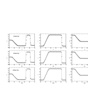
Figure 1: Density (left), velocity (center) and pressure (right) for the Sod shock tube tests in one-, two- and three-dimensions. Open circles are given by the numerical solution output at $t=0.195$ using the fifth order WENO scheme, solid lines represent the analytical solutions.

The Sod shock tube is actually a 1-dimensional problem. To find how well the shock structure is resolved in high dimensions, we perform the test in one-, two- and three-dimensional cases. In 1-dimension, the shock propagates along the line of the x-axis. For two- and three-dimensional cases, the shock propagates along the main diagonal of the calculation region, i.e., along the line (0,0) to (1,1) in the square and along the line (0,0,0) to (1,1,1) in the cube. Fig. 1 compares the numerical results at $t=0.195$ with the analytical solution in one-, two- and three-dimensions respectively, in which 64 cells in each direction have been used. Comparable to the calculations done with PPM or TVD schemes (e.g. Ryu et al. 1993, Pen 1998, Ricker et al., 2000), the shock and contact discontinuity can be resolved within two to three cells in the multidimensional calculations, and moreover, each quantity gets some improvements with the increase of spatial dimensions.

4.2 Spherical Sedov-Taylor Blast Wave

Another challenging test for the 3-dimensional hydrodynamic code is the Sedov blast wave (Sedov, 1993). We initialize the simulation by setting up a point-like energy release in a homogeneous medium of density and negligible pressure. This explosion will develop a spherical blast wave that sweeps material around as it propagates outward along the radial direction. The derivation of the full analytical solutions can be found in Landau & Lifshitz (1987). It has been currently used for modeling the supernova explosion.

The shock front propagates according to

$$r_{s}(t)=\xi_{0}\left(\frac{E_{0}t^{2}}{\rho_{1}}\right)^{1/5}$$ (14)

where $\xi_{0}=1.15$ for an ideal gas with a polytropic index $\gamma=5/3$. The velocity of the shock is given by $v_{s}=\partial r_{s}(t)/\partial t$. Behind the shock, the density, momentum and pressure are given by

$$\rho_{2} = \frac{\gamma+1}{\gamma-1}\rho_{1}$$ (15)

$$(\rho v)_{2} = \frac{2}{\gamma-1}\rho_{1}v_{s}$$ (16)

$$P_{2} = \frac{2}{\gamma+1}\rho_{1}v_{s}^{2}.$$ (17)

We apply the 3-dimensional WENO scheme to run the Sedov-Taylor blast test. The simulation is performed in a cubic box with a $256^{3}$ grid, and initialized by setting up a uniform density $\rho_{1}=1$ and negligible pressure with a very small value $p_{0}=10^{-5}$ to match a numerical approximation to zero. A point-like energy $E_{0}=10^{5}$ is injected at the center of the box, and the medium is at rest initially. The challenging nature of the spherical Sedov-Taylor blast wave stems from the fact that a Cartesian grid is used. To minimize the anisotropic effects due to the Cartesian coordinates, we convolve the initial condition with a spherical Gaussian filter with a window radius of 1.5 grids.

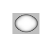
Figure 3: The gray image of density distribution in a slice across the explosion point in the three-dimensional spherical Sedov blast wave at t=9.22.

The full three-dimensional numerical solutions for density, momentum and pressure are displayed in Fig. 2 by projecting onto the radial coordinate. As can be seen in Fig. 2, the numerical solution captures the spatial profile of the shock well, although there is still some scattering around the analytical solution. Obviously, the scattering originates from the geometric effect of the projection from the Cartesian grid onto the spherical coordinate. Such geometric anisotropy also leads to the shock front being not fully resolved within one cell as described by the analytical solution. Accordingly, in the widened shock front of the numerical solution, both density and pressure have been underestimated in comparison with their predicted maximum values. Fig. 3 presents the density distributions in a slice across the explosion point. The anisotropy could be clearly seen in this figure.

4.3 Zeldovich Pancake

The Zeldovich pancake problem (Zeldovich, 1970) provides a stringent numerical test for cosmological hydrodynamic codes. It involves the basic physics underlying in cosmological simulation, namely, hydrodynamics, self-gravity, cosmic expansion, and strong shock formed in smooth structure with high Mach numbers. In the one-dimensional case, the problem can be formulated by placing a sinusoidal perturbation along the axis and tracking its evolution. In the linear or quasi-linear regime, there exists an exact solution in the Lagrangian coordinate if the pressure is neglected. For a flat cosmology, the solution can be written in the following forms

$$\rho(x_{l}) = \rho_{0}\Big{[}1-\frac{1+z_{c}}{1+z}\cos(kx_{l})\Bigr{]}^{-1}$$ (18)

$$v(x_{l}) = -H_{0}\frac{1+z_{c}}{(1+z)^{1/2}}\frac{\sin(kx_{l})}{k}$$ (19)

where $z_{c}$ is a redshift at which the gravitational collapse results in the formation of caustics, i.e., Zeldovich pancake. $H_{0}$ is the Huuble constant, $H_{0}=100hkm/s/Mpc$, and $k=2\pi/\lambda$ specifies the comoving perturbation wavelength. $x_{l}$ is the Lagrangian coordinate which is related to the Eulerian position $x_{e}$ by

$$x_{l}-\frac{1+z_{c}}{1+z}\frac{\sin(kx_{l})}{k}=x_{e}.$$ (20)

For the numerical model, we adopt the same parameters as those used in Bryan et al. (1995), which are given by $z_{c}=1$, $\Omega=1$ , $h=0.5$, $\lambda=64h^{-1}Mpc$. The simulation is performed from the initial redshift $z_{i}=100$ for the purely baryonic gas with a uniform temperature distribution $T_{i}=100K$.

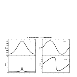
Figure 4: The one-dimensional Zeldovich Pancake test at redshifts z=10 and z=1.05 prior to the caustics formation. The results from a 256 grids run (open circle) are plotted against the exact solutions (solid line).

It is noted that the analytical solution given by equation (18) holds until the redshift $z=z_{c}$ of caustic formation. In Fig. 4, we compare the numerical solution using a $256$ grid to the Zeldovich pancake with the analytical solution at z=10 and z=1.05. We can clearly see an excellent agreement between the numerical and analytical solutions. To access the accuracy to which our WENO/PM code is able to reach, we run the code with a fixed perturbation wavelength but a varying number of zones $N$. Using the exact solution (16)-(18), we define the $L^{1}$ error norms for the density as

$$\Delta\rho=\frac{1}{N}\sum_{i=1}^{N}|\frac{\rho_{i}-\rho_{zel,i}}{\rho_{zel,i}}|$$ (21)

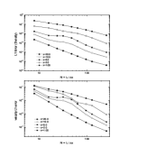
Figure 5: The $L^{1}$ error norm of one-dimensional Zeldovich pancake tests varying with the number of zones $N$ for a fixed perturbation wavelength. The results for density (upper panel) and velocity (lower panel) are plotted at different redshifts.

where $\rho_{i}$ is the numerical solution on the grid, and $\rho_{zel,i}$ is the Zeldovich solution given by equation (16). The $L^{1}$ error norm for the velocity fields are defined similarly. The results at different redshifts ranging from the linear regime $z=20$ to the highly nonlinear collapsing phase $z=1.05$ are displayed in Fig. 5. Usually, the $L^{1}$ error should be scaled with $N$ according to a power law $\sim N^{-r}$ or with spatial resolutions as ${\Delta x}^{r}$, where $r$ is defined as the convergence rate. For the density field, the $L^{1}$ error declines rapidly with $r\simeq 1.8$ at $z=20$. With decreasing redshifts, the convergence rate slows down, e.g., the error varies approximately as $N^{-1}$ at $z=1.05$, namely, roughly a linear convergence law with the spatial resolution. The velocity at $z=20$ converges somewhat faster than the density with convergence rate $r\simeq 1.9$, but somewhat slower at $z=1.05$ with $r\simeq 0.9$.

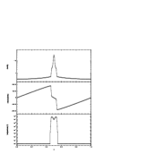
Figure 6: The density (top), velocity (middle) and temperature (bottom) for a one-dimensional Zeldovich pancake at redshift z=0. The results are drawn from a 256 grid run.

The non-linear evolution subsequent to the caustics formation is more difficult to track numerically than that in the linear phase. The formation of the caustics is due to the head-on collision of two cold bulk flows and gravitational collapsing, which result in a strong shock and large gradients in the involved physical fields. Moreover, a large range of variation in the temperature distribution is also difficult to capture numerically. In Fig. 6 we plot the solution for the density, velocity and temperature distribution at $z=0$ obtained from a 256 zone run. It should be noted that, in the unshocked region, the temperature is solved from the entropy equation and remains with a uniform temperature 1K, which is the artificial minimum temperature.

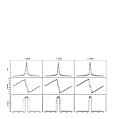
Figure 7: The density (top), velocity (middle) and temperature (bottom) for a one-dimensional Zeldovich pancake at redshift z=0. Open circles with dotted lines are obtained from the runs with 32, 64, 128 grids. The solid lines are for the solution computed with a 512 grid run.

To determine how well the shock is resolved by the WENO scheme at different resolutions, we also make runs with 32, 64, 128 zones and compare with a high resolution run with 512 zones. Unlike the similar comparison done by Bryan using the PPM scheme, we have not degraded the solution at the high resolution to appropriate scales. The results are shown in Fig. 7. Clearly, the shock structure is well resolved by approximately equal number of zones for the three low resolution solutions, although the width of the shock is widened with reduced resolution correspondingly. Moreover, we see that the solution with 128 zones has already converged to that with 512 zones, which is likely to be the real physical solution to the problem. This demonstrates the rapid convergence rate of the high order WENO scheme even in the highly nonlinear phase of the caustics.

4.4 A Cosmological Application: the $\Lambda$CDM Model

We run the hybrid hydrodynamic/N-body WENO/PM code to track the cosmic evolution of the coupled system of both dark matter and baryonic matter in a flat low density CDM model ($\Lambda$CDM), which is specified by the density parameter $\Omega_{m}=0.3$, cosmological constant $\Omega_{\Lambda}=0.7$, Hubble constant $h=0.7$, and the mass fluctuation within a sphere of radius 8h^-1Mpc, $\sigma_{8}=0.9$. The baryon fraction is fixed using the constraint from primordial nucleosynthesis as $\Omega_{b}=0.0125h^{-2}$ (Walker et al., 1991). The initial condition has been generated by the Gaussian random field with the linear CDM power spectrum taken from the fitting formulae presented by Eisenstein & Hu (1998). The simulation is performed in a periodic box of side length of 25h^-1Mpc with a 192³ grid and an equal number of dark matter particles. The universe is evolved from $z=49$ to $z=0$. The initial temperature is set to $T=10^{4}K$ and the polytropic index takes the value $\gamma=5/3$. For comparison, two sets of simulation have been performed by using the WENO-E and WENO-S schemes, which update the energy and entropy respectively outside the shocked regions, see section 3.3.

Fig. 8 plots density contours for the baryonic matter (lower panel) and the cold dark matter (upper panel) in a slice with 2-cell thickness of 0.26h^-1Mpc at $z=1.5$. In Fig. 9, we compare the cell temperature contours drawn from the simulations using the WENO-E (lower panel) and WENO-S (upper panel) codes. Obviously, the two simulations coincide in the high temperature $(>10^{4}K)$ regions, but in the low temperature regions, the WENO-E simulation gives less fractions of the volume than those from WENO-S. This phenomenon is due to the artificial numerical errors, which heats up significantly the regions with temperature $\leq 10^{2}$K to $T\sim 10^{2}-10^{4}$K in the WENO-E calculation. In contrast, since the entropy equation is capable of tracking the temperature field with high accuracy and hence the spurious heating is minimized, the cold unshocked regions occupy more volumes in the WENO-S calculation.

Fig. 10 gives an example of density, velocity and temperature distributions along a randomly chosen lines of sight. To demonstrate further the difference between the WENO-E and WENO-S codes, we plot the results from both calculations in each panel. Once again, the numerical heating in the pre-shock or unshocked regions is clearly seen in this plot. Our result is compatible with that of Ryu et al. (1993) for a purely baryonic universe. Moreover, it is also noted from Fig. 10 that there are not significant differences between the density and velocity fields in the WENO-S and WENO-E calculations, while for the temperature distribution, the difference occurs in the regions of cold gas, $T\leq 10^{4}$K. This demonstrates that the internal energy corrections made in cold regions (mostly in unshocked gas) by the modified entropy equation have little dynamical effect on the flow structure except for the internal energy or temperature fields.

In Fig. 11, we present an alternative view of the difference between the WENO-E and WENO-S codes by plotting histograms of the volume-weighted (upper panel) and mass-weighted (lower panel) temperature on the $192^{3}$ grids. Clearly, the artificial numerical heating is serious in the regions occupied by the low-temperature gas in the WENO-E calculation, however it is less significant in the fraction of mass. Another illustration indicating such a difference can be given by contour plots of the volume fraction with given temperature and density. As displayed in Fig. 12, the volume difference only occurs in the low-density/low temperature regions with $\rho/\bar{\rho}\leq 1$ and $T\leq 10^{4}$K, typically around $\rho/\bar{\rho}\sim 0.1$, $T\sim 10^{3}$K. It should be noted that, although the spurious heating does exist also in the standard WENO code, it is weaker than those in low-order schemes, e.g., the second order TVD code of Ryu et al. (1993). This benefit clearly comes from the higher order accuracy acquired in our fifth-order WENO scheme, which leads to smaller numerical errors in the calculations. However, for realistic cosmological simulations, such a difference may not be significant while the radiation field is taken into account. For instance, in the presence of ionizing UV background, the baryonic intergalactic medium could be heated up to $\sim 10^{4}$K. The simulation including the radiative heating-cooling and ionization and relevant statistical analysis will be presented elsewhere.

5 Concluding Remarks

In this paper, we have described a newly developed hybrid cosmological hydrodynamic code based on weighted essentially non-oscillatory (WENO) schemes for the Euler system of conservation laws. We implement the fifth order finite difference WENO to solve the inviscid fluid dynamics on a uniform Eulerian grid combining with a third order low storage Runge-Kutta TVD scheme for advancing in time. In order to solve the cosmological problem involving both collisional baryonic matter and collisionless dark matter, we incorporate the particle-mesh method for computing the self-gravity into our cosmological code.

The code has been subjected to a number of tests for its accuracy and convergence. As expected, the WENO scheme demonstrates its capacity of capturing shocks and producing sharp and non-oscillatory discontinuity transition without generating oscillations. In comparison with other existing hydrodynamic codes such as the TVD or PPM schemes, one striking feature of the WENO code is that it retains higher order accuracy in smooth regions including at smooth extrema even in multidimensions, and yet it is still highly stable and robust for strong shocks. In performance, the WENO scheme needs more floating point operations per cell than those of the PPM and TVD schemes. However, in compensating for twice or more loss of the computational speed, the WENO scheme achieves both higher order accuracy and convergence rate than PPM and TVD codes according to our numerical tests.

In the presence of gravity, the hydrodynamics become more challenging than that without gravity due to the highly non-linearity of gravitational clustering. One serious problem encountered in many cosmological applications is the so called high Mach number problem. To address this problem, we have incorporated an extra technique into our cosmological WENO/PM code, which is actually a combination of the dual energy algorithm (Bryan et al. 1995) and the energy-entropy algorithm (Ryu et al. 1993). Namely, instead of solving the internal energy equation in regions free of shocks as was done in the dual energy algorithm (Bryan et al. 1995), we solve the modified entropy equation (Ryu et al. 1993), which takes a conservative form and can be easily solved using the standard WENO scheme. This improvement over our hydrodynamic WENO code ensures an accurate tracking of the temperature field in regions free of shocks.

It is pointed out that the high order WENO discretization, e.g., the fifth order WENO scheme adopted in this paper, introduces a quite small numerical viscosity, which does not lead to a significant violation of energy conservation in the presence of gravitational fields. While for a second-order TVD scheme, the numerical diffusion is no longer negligible. In order to have a better conservation of the total energy, it is usually corrected by adding a compensation term in the gravitational force term (Ryu et al, 1993).

The Euler hydrodynamics on fixed meshes have several distinct advantages which includes simplicity for implementation, easy data parallelization, relatively low floating point cost, large dynamic range in mass and high resolution of shock capturing. In particular, the WENO scheme can also achieve a higher accuracy on coarse meshes and a better resolution on the largest meshes allowed by available memory. To suit for large simulations of the cosmological problem, further improvement of the hydrodynamic WENO code is needed in its implementation on distributed memory computers. The parallel version of the code based on the Message-Passing Interface (MPI) has been under development.

Appendix A Low Storage Runge-Kutta Scheme

General low-storage Runge-Kutta schemes can be written in the form

$$du^{(i)} = A_{i}du^{(i-1)}+\Delta tL(u^{(i-1)},t^{n}+\alpha_{i}\Delta t)$$

$$u^{(i)} = u^{(i-1)}+B_{i}du^{(i)},\qquad i=1,...,m$$ (A1)

$$u^{(0)} = u^{n},\,\,\,u^{(m)}=u^{n+1},\,\,\,A_{1}=0.$$

Only $u$ and $du$ must be stored, resulting in two storage units for each variable, instead of three storage units for equation (3.2). The third order nonlinearly stable version we use, Gottlieb & Shu (1998), has $m=3$ in (A) with

$$z_{1} = \sqrt{36c_{2}^{4}+36c_{2}^{3}-135c_{2}^{2}+84c_{2}-12}$$

$$z_{2} = 2c_{2}^{2}+c_{2}-2$$

$$z_{3} = 12c_{2}^{4}-18c_{2}^{3}+18c_{2}^{2}-11c_{2}+2$$

$$z_{4} = 36c_{2}^{4}-36c_{2}^{3}+13c_{2}^{2}-8c_{2}+4$$

$$z_{5} = 69c_{2}^{3}-62c_{2}^{2}+28c_{2}-8$$

$$z_{6} = 34c_{2}^{4}-46c_{2}^{3}+34c_{2}^{2}-13c_{2}+2$$

$$B_{1} = c_{2}$$ (A2)

$$B_{2} = \frac{12c_{2}(c_{2}-1)(3z_{2}-z_{1})-(3z_{2}-z_{1})^{2}}{144c_{2}(3c_{2}-2)(c_{2}-1)^{2}}$$

$$B_{3} = \frac{-24(3c_{2}-2)(c_{2}-1)^{2}}{(3z_{2}-z_{1})^{2}-12c_{2}(c_{2}-1)(3z_{2}-z_{1})}$$

$$A_{2} = \frac{-z_{1}(6c_{2}^{2}-4c_{2}+1)+3z_{3}}{(2c_{2}+1)z_{1}-3(c_{2}+2)(2c_{2}-1)^{2}}$$

$$A_{3} = \frac{-z_{4}z_{1}+108(2c_{2}-1)c_{2}^{5}-3(2c_{2}-1)z_{5}}{24z_{1}c_{2}(c_{2}-1)^{4}+72c_{2}z_{6}+72c_{2}^{6}(2c_{2}-13)}$$

$$\alpha_{1} = 0$$

$$\alpha_{2} = B_{1}$$

$$\alpha_{3} = B_{1}+B_{2}(A_{2}+1)$$

where $c_{2}=0.924574$.

Figure 2: The density (top), momentum density (middle) and pressure (bottom) in the three-dimensional spherical Sedov blast wave test at t=9.22. The computation was performed on a $256^{3}$ grid, and the scattered points are plotted by the projection of the results on the Cartesian grids onto the spherical radial coordinates. The solid lines represent the analytical solutions.

Figure 8: Gas density (lower panel) and CDM density (upper panel) contour plots for a slice of 0.26h^-1Mpc thickness in a 192³ grid at $z=1.5$. The solid line contours represent overdense regions with $\rho/\bar{\rho}\geq 1$, and the dotted lines represent underdense regions with $\rho/\bar{\rho}\leq 1$.

Figure 9: Comparison of temperature contours for the WENO-E (lower panel) and WENO-S (upper panel) for a slice of 0.26h^-1Mpc thickness in a 192³ grid at $z=1.5$. The solid line contours represent hot regions with $T\geq 10^{4}$K and the dotted lines represent cold region with $T<10^{4}$K.

Figure 10: Density, velocity and temperature distributions along a randomly chosen lines of sight at $z=1.5$. The solid lines are for the WENO-S simulation and the dotted lines for the WENO-E simulation.

Figure 11: The cell temperature histogram in a 192³ grid at $z=1.5$. The top panel is for the volume-weighted cell temperature and the lower panel for the mass-weighted cell temperature. In both panels, the solid lines are given by the WENO-S simulation and the dotted lines given by the WENO-E.

Figure 12: Contour plot of the volume with given temperature and density at $z=1.5$. The left panel is for the calculation with the WENO-E and the right panel with the WENO-S.

References

- (1)
- (2) Balsara, D., & Shu, C.-W., 2000, J. Comput. Phys., 160, 405
- (3)
- (4) Bertschinger, E., 1998, ARA&A, 36, 599
- (5)
- (6) Bryan, G.L., Norman, M.L., Stone, J.M., Cen, R., & Ostriker, J.P., 1995, Comput. Phys. Comm., 89, 149
- (7)
- (8) Cen, R., 1992, ApJS, 78, 341
- (9)
- (10) Colella, P., & Woodward, P.R., 1984, J. Comp. Phys., 54, 174
- (11)
- (12) Couchman, H.M,P., Thomas, P.A., & Pearce, F.R., 1995, ApJ, 452, 797
- (13)
- (14) Efstathiou, G., Davis, M., Frenk, C.S., & White, S.D.M., 1985, ApJS, 57, 241
- (15)
- (16) Eisenstein, D.J., & Hu, W., 1999, ApJ, 511, 5
- (17)
- (18) Evrard, A.E., 1988, MNRAS, 235, 911
- (19)
- (20) Giacconi, P., Gursky, H., Paolini, F., & Rossi, B., 1962, Phys. Rev. Lett., 9, 439
- (21)
- (22) Gingold R.A. & Monaghan, J.J., 1977, MNRAS, 181, 375
- (23)
- (24) Gnedin, N.Y., 1995, ApJS, 97, 231
- (25)
- (26) Gottlieb, S., & Shu, C.-W., 1998, Math. Comp., 67, 73
- (27)
- (28) Gottlieb, S., Shu, C.-W., & Tadmor, E., 2001, SIAM Review, 43, 89
- (29)
- (30) Grasso F., & Pirozzoli, S., 2000a, Theor. Comp. Fluid Dyn., 13, 421
- (31)
- (32) Grasso, F., & Pirozzoli, S., 2000b, Phys. Fluids, 12, 205
- (33)
- (34) Hernquist, L., & Katz, N., 1989, ApJS, 70, 419
- (35)
- (36) Harten, A., 1983, J. Comput. Phys., 49, 357
- (37)
- (38) Harten, A., Engquist, B., Osher, S.J., & Chakravarthy, S., 1987, J. Comput. Phys., 71, 231
- (39)
- (40) Hockney, R.W., & Eastwood, J.W., 1988, Computer Simulation Using Particles (Philadelphia: IOP Publishing)
- (41)
- (42) Jiang, G., & Peng, D.P., 2000, SIAM J. Sci. Comput., 21, 2126
- (43)
- (44) Jiang, G., & Shu, C.-W., 1996, J. Comput. Phys., 126, 202
- (45)
- (46) Jiang, G., & Wu, C.-C. 1999, J. Comput. Phys., 150, 561
- (47)
- (48) Landau, L.D., & Lifshitz, E.M., 1987, Fluid Mechanics (2nd ed.; Oxford: Pergamon Press)
- (49)
- (50) Liang, S., & Chen, H., 1999, AIAA J., 37, 1010
- (51)
- (52) Liska, R., & Wendroff, B., 1998, SIAM J. Numer. Anal., 35, 2250
- (53)
- (54) Liska, R., & Wendroff, B., 1999, Int. J. Numer. Meth. Fl., 30, 461
- (55)
- (56) Liu, X.D., Osher, S.J., & Chan, T., 1994, J. Comput. Phys., 115, 200
- (57)
- (58) Lucy, L.B., 1977, ApJ, 82, 1013
- (59)
- (60) Montarnal, P., & Shu, C.-W., 1999, J. Comput. Phys., 148, 59
- (61)
- (62) Mulchaey, J.S., 2000, ARA&A, 38, 289
- (63)
- (64) Navarro, J.F., & White, S.D.M., 1993, MNRAS, 265, 271
- (65)
- (66) Noelle, S., 2000, J. Comput. Phys., 2000, 283
- (67)
- (68) Norman, M.L., & Bryan, G.L., 1999, in Numerical astrophysics, 1998, ed. S. Miyama, K. Tomisaka, & T. Hanawa (Boston: Kluwer)
- (69)
- (70) O’Shea, B.W., Bryan, G., Bordner, J., Norman, M.L., Abel, T., Harkness, R., & Kritsuk, A., 2004, in Adaptive Mesh Refinement - Theory and Applications, eds. Plewa, T., Linde T. & Weirs, V.G. (Springer)
- (71)
- (72) Ostriker, J.P. & Vishniac, E.T., 1986, ApJ, 306, L51
- (73)
- (74) Owen, J.M., Villumsen, J.V., Shapiro, P.R., & Martel, H., 1998, ApJS, 116, 155
- (75)
- (76) Pen, U.L., 1998, ApJS, 115, 19
- (77)
- (78) Rauch, M., 1998, A&A, 36, 267
- (79)
- (80) Ricker, P.M., Dodelson, S. & Lamb, D.Q., 2000, ApJ, 536, 122
- (81)
- (82) Roe, P., 1978, J. Comput. Phys., 27, 1
- (83)
- (84) Ryu, D., Ostriker, J.P., Kang, H. & Cen, R.,1993, ApJ, 414, 1
- (85)
- (86) Sedov, L.I., 1993, Similarity and Dimensional Methods in Mechanics (Boca Raton, CRC press, 10th ed.)
- (87)
- (88) Shi, J., Zhang, Y.T. & Shu, C.-W., 2003, J. Comput. Phys., 186, 690
- (89)
- (90) Shu, C.-W., 1988, SIAM J. Sci. Stat. Comput., 9, 1073
- (91)
- (92) Shu, C.-W., 1998, in Advanced Numerical Approximation of Nonlinear Hyperbolic Equations, B. Cockburn, C. Johnson, C.-W. Shu and E. Tadmor (Editor: A. Quarteroni), Lecture Notes in Mathematics, 1697, 325 (Springer)
- (93)
- (94) Shu, C.-W., 1999, in High-Order Methods for Computational Physics, T.J. Barth and H. Deconinck, editors, Lecture Notes in Computational Science and Engineering, 9, 439 (Springer)
- (95)
- (96) Shu, C.-W., 2003, Int. J. Comput. Fluid Dyn., 17, 107
- (97)
- (98) Shu, C.-W. & Osher, S.J., 1988, J. Comput. Phys., 77, 439
- (99)
- (100) Sod, G.A., 1978, J. Comput. Phys., 27, 1
- (101)
- (102) Sornborger, A., Fryxell, B., Olson, K. & MacNeice, P., 1996, preprint (astro-ph/9608019)
- (103)
- (104) Springel V., Yoshida N., & White S.D.M., 2001, New Astronomy, 6, 51
- (105)
- (106) Steinmetz, M., 1996, MNRAS, 278, 1005
- (107)
- (108) Stone J.M., & Norman, M.L., 1992, ApJS, 80, 753
- (109)
- (110) Teyssier, R., 2002, A&A, 285, 337
- (111)
- (112) Turner, M.S, 2002, ApJ, 576, L101
- (113)
- (114) Walker, T., Steigma, G., Schramm, D.N., Olive, K.A. & Kang, H.S., 1991, ApJ, 376, 51
- (115)
- (116) Yang, J., Yang, S., Chen, Y. & Hsu, C., 1998, J. Comput. Phys., 146, 464
- (117)
- (118) Zanna, L. Del, Velli, M. & Londrillo, P., 1998, A&A, 330, L13
- (119)
- (120) Zeldovich, Ya. B., 1970, A&A, 5, 84
- (121)
- (122) Zel’dovich, Ya. B., & Sunyaev, R.A., 1969, A&A, 20, 189
- (123)