Phase-Space Structure of Dark-Matter Haloes: Scale-Invariant PDF Driven by Substructure
Abstract
We present a method for computing the 6-dimensional coarse-grained phase-space density in an N-body system, and derive its distribution function . The method is based on Delaunay tessellation, where is obtained with an effective fixed smoothing window over a wide range. The errors are estimated, and is found to be insensitive to the sampling resolution or the simulation technique. We find that in gravitationally relaxed haloes built by hierarchical clustering, is well approximated by a robust power law, , over more than 4 decades in , from its virial level to the numerical resolution limit. This is tested to be valid in the CDM cosmology for haloes with masses , indicating insensitivity to the slope of the initial fluctuation power spectrum. By mapping the phase-space density in position space, we find that the high- end of is dominated by the “cold” subhaloes rather than the parent-halo central region and its global spherical profile. The value of in subhaloes near the virial radius is typically times higher than its value at the halo centre, and it decreases gradually from outside in toward its value at the halo centre. This seems to reflect phase mixing due to mergers and tidal effects involving puffing up and heating. The phase-space density can thus provide a sensitive tool for studying the evolution of subhaloes during the hierarchical buildup of haloes. It remains to be understood why the evolved substructure adds up to the actual universal power law of . It seems that this behaviour results from the hierarchical clustering process and is not a general result of violent relaxation.
keywords:
cosmology: theory — dark matter — galaxies: dwarfs — galaxies: formation — galaxies: haloes — galaxies: interactions — galaxies: kinematics and dynamics1 INTRODUCTION
The standard paradigm assumes that dark-matter haloes are the basic entities in which luminous galaxies form and live. The haloes dominate the gravitational potential over a wide range of radii and they have a crucial role in determining the galaxy properties. While many of the systematic features of halo structure and kinematics have been revealed by -body simulations, the origin of these features is still an open theoretical puzzle, despite the fact that they are due to simple Newtonian gravity.
The halo density profile is an example for such a puzzle. It is found in the simulations to have a robust non-power-law shape (which we refer to in general as “NFW”), with a log slope near the virial radius, flattening gradually toward at about 1% of the virial radius, and perhaps flattening further at smaller radii. (e.g. Navarro, Frenk & White, 1997; Moore et al, 1998; Klypin et al, 2001; Power et al, 2003; Hayashi et al, 2004, and references therein). This density profile is insensitive (or at most weakly sensitive) to parameters of the cosmological model and the initial fluctuation power spectrum (e.g., Cole & Lacey, 1996; Navarro, Frenk & White, 1997; Subramanian, Cen & Ostriker, 2000; Ricotti, 2003; Colín et al, 2003; Navarro et al, 2004) indicating that its origin is due to a robust relaxation process rather than specific initial conditions. In particular, violent relaxation (Lynden-Bell, 1967) may be involved in shaping up the density profile. In addition, secondary infall may be important in the outer regions (Gunn and Gott, 1972; Dekel, Kowitt & Shaham, 1981; Fillmore and Goldreich, 1984; Hoffman & Shaham, 1985; White & Zaritsky, 1992) while some argue that resonances may have a role in the inner regions (Weinberg & Katz 2002; but see Valenzuela & Klypin 2003). Nevertheless, there is no clear understanding for why the haloes actually pick up the particular density profile they have.
The properties of the velocity dispersion tensor is another theoretical puzzle. The haloes tend to be rather round, with a velocity dispersion profile that is slightly rising at small radii and slightly falling at large radii but is rather flat overall (Huss et al, 1999a, b). The profile of the anisotropy parameter , which is a measure of radial versus tangential velocities, indicates near isotropy at small radii, which gradually develops into more radial orbits at large radii (Cole & Lacey, 1996; Huss et al, 1999a, b; Colín et al, 2000a). For a spherical system in equilibrium, the and are related to via the Jeans equation, but it is not at all clear why the haloes in the simulations choose the characteristic or that they actually do.
An interesting attempt to address the origin of the halo profile has been made by Taylor & Navarro (2001), who measured a poor-man phase-space density profile by , and found that it displays an approximate power-law behaviour, , over more than two decades in . Using the spheri-symmetric Jeans equation, they showed that this power law permits a whole family of density profiles, whose limiting case is a profile similar to NFW, which asymptotically approaches a slope as . The general power-law shape of is confirmed in the simulated haloes described below. This scale-free behaviour of is intriguing, and it motivates further studies of halo structure by means of phase-space density.
Simulations of the CDM cosmology also reveal a roughly self-similar hierarchical clustering process, where smaller building blocks accrete and merge into bigger haloes. At every moment, every halo contains a substructure of subhaloes on top of a smooth halo component that has been tidally stripped from an earlier generation of substructure. Some of the important dynamical processes involved in this hierarchical halo buildup are understood qualitatively. These include, for example, the dynamical friction which governs the decay of the satellite orbits, the tidal stripping of subhaloes due to the host halo potential, and the mergers and flyby interactions of the subhaloes among themselves. However, a complete theoretical understanding of how these processes work in detail, and how they combine to produce the halo structure and kinematics, is lacking.
Attempts have been made to explain an inner density cusp using toy models of dynamical stripping and tidal effects during the halo buildup by mergers (Syer & White, 1998; Nusser & Sheth, 1999; Dekel, Devor & Hetzroni, 2003; Dekel et al., 2003). However, a similar halo density profile seems to be produced also in some of the simulations where substructure has been artificially suppressed (Moore et al., 1999b; Huss et al, 1999a; Avila-Reese et al., 2001; Bullock, Kravtsov & Colin, 2002; Alvarez, Shapiro & Martel, 2002), indicating that the process responsible for the origin of this density profile might be a somewhat more general feature of gravity and not unique to the merger scenario.
The issue of halo substructure has become timely both because of its relevance to observations and its implications on other major issues in galaxy formation. Tidal tails and streams associated with dwarf satellite galaxies have been observed in the haloes of the Milky Way and M31 (Ibata et al, 1994, 2001a, 2001b), and they start to allow detailed modelling of the halo history through the satellite orbits. Gravitational-lensing observations provide preliminary indications for the presence of substructure in haloes at the high level predicted by the dissipationless CDM scenario (e.g. Dalal & Kochanek, 2002) In contrast, the observed number density of dwarf galaxies seems to be significantly lower, thus posing a “missing dwarf problem” Klypin et al. (1999b); Moore et al (1999a). Also, the “angular-momentum problem” of disk galaxies (e.g. Navarro & Steinmetz, 2000; Bullock et al., 2001b) is probably associated with the evolution of substructure in haloes (Maller & Dekel, 2002; Maller, Dekel & Somerville, 2002). While the dwarf and angular-momentum problems necessarily involve baryonic processes, understanding the gravitational evolution of substructure is clearly a key for solving them.
In order to better understand the origin the various aspects of halo structure and buildup mentioned above, we make here a first attempt at addressing directly and in some detail the phase-space structure of dark-matter haloes. The fundamental quantity in the dynamical evolution of gravitating systems is the full, six-dimensional, coarse-grained, phase-space density , which intimately relates to the underlying Vlasov equation and lies behind any relaxation process that may give rise to the virialized halo structure (Binney & Tremaine, 1987, chapter 4).
Ideally, one would have liked to compute it free of assumptions concerning spherical symmetry, isotropy, or any kind of equilibrium. However, computing densities in a six-dimensional space is a non-trivial challenge which requires simulations of a very broad dynamical range. The state-of-the-art N-body simulations, with more than million particles per halo, allow an attempt of this sort for the first time. We describe below a successful algorithm for measuring , and study its relevant properties including the associated systematic and random uncertainties. We then apply this algorithm to simulated virialized haloes in the CDM cosmology.
We report in this paper two surprising new results. First, we discover that the volume distribution function of the phase-space density, , displays a universal scale-invariant power-law shape, valid in all virialized haloes that form by hierarchical clustering. Second, we realise that this power law is not directly related to the overall density profile, but is rather driven by the halo substructure. This implies that the phase-space density provides a useful tool for studying the hierarchical buildup of dark-matter haloes and the evolution of substructure in them.
In §2 we introduce and . In §3 we describe the method of computing and from an -body halo, and summarise its properties and the associated errors, which are addressed in more detail in Appendix A. In §4 we present the universal power-law shape of based on several different simulations, and demonstrate its robustness to the mass scale and simulation technique. In §5 we display maps of phase-space density and show that the high- contributions to come from substructures within the parent halo. In §6 we summarise and discuss our results and future work.
2 THE PDF OF PHASE-SPACE DENSITY:
This is a more technical and elaborate introductory section, aimed at introducing the concepts and nomenclature relevant for the analysis of this paper.
2.1 Definitions
The state of a collisionless system is completely determined by the fine-grained phase-space density function , which measures the mass contained in an infinitesimal phase-space patch of volume , located at . The evolution of is governed by the Vlasov equation,
| (1) |
with the gravitational potential, related self-consistently to by the Poisson’s integral
| (2) |
It is therefore sensible to assume that a true understanding of the nature of self-gravitating collisionless systems must involve as a primary ingredient. However, being a function of six variables, is hard to deal with computationally. It turns out that there is a much simpler function, , which is intimately related to , but is much easier to handle both analytically and numerically.
Before defining , it is worth recalling that the Vlasov equation preserves the phase-space density along particle trajectories: It implies eq. (1) implies that
| (3) |
where is the trajectory of a phase-space element. This conservation of phase-space density along trajectories can also be viewed as a conservation of phase-space volume. In order to illustrate what this means, consider any smooth function , and define the integral
| (4) |
Using the Vlasov equation we find that
| (5) | |||||
| (6) | |||||
| (7) |
The last equality follows by integrating the first term over and the second term over , and assuming that as . This implies that is conserved under the dynamics.
Now, if is the Dirac delta function111Strictly speaking, the Dirac delta function is not a smooth function, but it can be approximated by a series of smooth functions, each obeying Eq. (7) , then the integral becomes an -dependent function, which we refer to as the PDF :
| (8) |
From this definition it is clear that is the volume of phase-space occupied by phase-space elements whose density lies in the range . The conservation of implied by Eq. (7) means that this volume is conserved under the dynamics. The fine-grained [i.e., the which is calculated using the fine-grained ] should therefore be viewed as a signature of the system, which remains the same throughout its evolution.
2.2 Coarse-Grained Density and Mixing
One might have thought that the conservation of poses severe constrains on the evolution of , but this is not the case due to the effects of mixing. In the course of evolution, phase-space patches of high are stretched and spiral into regions with low . As the stretching continues, the patches become thiner and thiner, and as a result varies over increasingly smaller scales. Very soon, one can no longer measure , but instead measure an average of it over some finite volume. This average is often referred to as the “coarse-grained” phase-space density, as opposed to the original “fine-grained” density . We denote the coarse-grained quantities by and , but in subsequent sections we may omit the bar and simply refer to them as and . The important point to realise is that the coarse-grained is no longer conserved. For example, given initially a volume filled with phase-space density and a similar volume filled with density , one ends after mixing with a volume filled with an average density .
When a large fraction of the mass is added to halo, e.g. by collapse or a major merger, rapid global fluctuations of the gravitational potential re-distribute the energies of each phase-space element, and lead to very strong mixing across large scales, resulting in variations in . After a few global dynamical times, the potential fluctuations fade away and stabilises. The fine-grained , on the other hand, continues to spiral and stretch indefinitely, on smaller and smaller scales, which no longer affect . After a while, the can be viewed as the “physical” phase-space density of the system, since the microscopic fluctuations of can no longer be measured, and, in particular, no longer affect the gravitational potential. It is therefore the coarse-grained which, according to Jeans’ theorem, can be written as a function of he invariants, the energy and the angular momentum . This relaxation process is referred to as violent relaxation (Lynden-Bell, 1967).
What is the coarse-grained of a relaxed system, and how is it related to the constant fine-grained of that system? One may identify the fine-grained with the coarse-grained at an early time when the initial is smooth enough not to vary over scales smaller than the averaging scale associated with . Then, the question can be rephrased in terms of the relation between the final and the early . One obvious constraint on the final , as an average of , is that their maximum values should obey . In particular, if the early [namely ] vanishes for , then so does the final .
The mixing theorem (Tremaine, Hénon & Lynden-Bell, 1986) specifies several additional constraints on the final , which arise from the fact that it has originated from a given . The cumulative distribution function is defined by
| (9) |
where is the Heaviside step function. As a monotonic function, can be inverted to yield , the reduced distribution function. The associated cumulative mass function , which measures the mass in phase-space regions where , is then defined by
| (10) | |||||
| (11) |
Substituting inside , one obtains the function , which can also be written as
| (12) |
If and denote the functions arising from the density functions and respectively, then the mixing theorem states that the final (coarse-grained) is an average of the initial (coarse- or fine-grained) if and only if for every . This, in turn, implies an implicit constraint on the evolution of the coarse-grained . This is one of the very few rigorous results concerning the evolution of , but its strength is rather limited because it provides only an integro-differential inequality that constrains .
The mixing theorem can be also stated directly in terms of , as shown by Mathur (1988). In his formulation, a necessary condition for the final (coarse-grained) evolved from the initial is that222This is the original statement in Mathur (1988). However, we believe that by adding the (trivial) condition that for every , it becomes also a sufficient condition.
| (13) |
with being some continuous function (not to be confused with a probability distribution) such that for all and for .
In the CDM scenario, the dark matter is initially cold – with vanishing velocity dispersion. This means a one-to-one correspondence between the particle positions and their velocities, , and the initial (fine-grained) phase-space density can be written as
| (14) |
Thus, in the beginning, the system can be described by the evolution of its density and velocity fields, often approximated by the Zel’dovich approximation. This singular nature of the initial phase-space density, together with its conservation, plays a crucial role in the formation of structures, and in particular in the abundance of dwarf haloes, and in the formation of cusps in dark-matter haloes (e.g. Colín et al, 2000b).
Physically, the phase-space density is never really infinite, as it is defined by a finite number of dark-matter particles per given phase-space volume. Numerically, it is the finite mass-resolution of the -body simulation that prohibits the phase-space density from being infinite. Therefore, the initial phase-space density is expected to be extremely high in regions where and vanishingly small elsewhere. Accordingly, will have contributions from a narrow range of extremely high values of and from a narrow range near . As the system evolves and mixing takes place, phase-space densities from both regions mix and give rise to intermediate values of , widening the distribution under the constraints of the mixing theorem.
2.3 A Relation Between and
In general, different systems may have the same . However, if the system is spherically symmetric and stationary, such that is a function of the energy alone, , then there is a unique relation between , and . We shall see in §4 that the measured in -body haloes is actually different from the one would have predicted from the halo using the relation assuming .
For a spherical system the relation between and can be derived as follows. Assume that , where , and define the density-of-states function
| (15) |
The quantity measures how much phase-space volume is occupied by phase-space elements with energy in the interval . When the system is spherical, can be written as (Binney & Tremaine, 1987, Eq. 4-157b),
| (16) |
with the inverse function of the gravitational potential. The overall phase-space volume occupied by energy levels below is thus given by
| (17) | |||||
| (18) |
Therefore, if is the cumulative defined in Eq. (9), and is a function of the energy alone, we obtain an integro-differential equation for :
| (19) |
This has to be supplemented by the equation that connects to (Binney & Tremaine, 1987, eq. 4-104),
| (20) | |||||
| (21) |
In general, these equations can be solved numerically, e.g., using a Picard iteration scheme.
In the asymptotic regime, the above equations can be solved analytically. If as , then, for , one can show that and have the scale-invariant forms
| (22) | |||||
| (23) |
Note that the derivative of Eq. (19) with respect to yields
| (24) |
By plugging the scale-invariant solutions of eq. (23) into eq. (24), one finds that for , the PDF is also a power law, , with
| (25) |
We learn that the density slopes in the range , relevant for the inner regions of haloes where is high, correspond to a narrow range of values, . In this case of power-law profiles, corresponds to the singular isothermal sphere , corresponds to an cusp, and corresponds to a flat core, .
Eq. (25) can also be obtained from simpler dimensional arguments using the virial theorem.
3 MEASURING IN AN -BODY SYSTEM
We wish to measure the phase-space density of a system represented by particles of mass each. One straightforward approach would have been to divide phase-space into a large number of Cartesian cells of equal volume each. If cell contains particles, then the average phase-space density in it can be estimated as . However, this approach is impractical in a six-dimensional space. A moderate resolution of 100 bins along each axis would require cells, which is beyond the capacity of any present-day computer. Moreover, for the computed to have any statistical meaning, there should be at least 100 particles in each cell (for a relative Poisson error of ), which requires a total of particles – about 5 orders of magnitude beyond the number of particles in today’s largest simulations.
A possible way to overcome this problem is by using an adaptive grid, where the cells vary in size to properly allow high resolution in high-density regions and low resolution in low-density regions. One can simply create an adaptive grid by dividing each Cartesian cell which contains more particles than some prescribed threshold into two or more sub-cells. This division can be done recursively until all cells contain particles or less.
Even more effective would be to vary the shape of the cells as well, allowing them to adapt more efficiently to the geometry of the underlying distribution and thus increase the effective resolution. A particularly robust method of this type is the Delaunay Tessellation Field Estimator (DTFE), which has already been implemented in three dimensions in a cosmological context (e.g. Bernardeau & van de Weygaert, 1996; Schaap & van de Weygaert, 2000, and references therein). We use this method here to measure in six dimensions.
3.1 Constructing a Delaunay Tessellation
A tessellation is the division of space into a complete covering of mutually disjoint convex polygons. The Delaunay tessellation (Delaunay, 1934) is defined for a sample of points as follows. The Delaunay cells that construct the tessellation are the -dimensional polyhedrons made by connecting every set of points whose circumsphere [the -dimensional sphere that passes through all of them] does not encompass any other point from the sample. One immediate advantage of the Delaunay tessellation is that it is parameter-free, and it completely adapts itself to the underlying distribution of points. Schaap & van de Weygaert (2000) have demonstrated the superiority of the DTFE over more conventional methods for estimating the density in 3D (methods like cloud-in-cell or the smoothing kernel used in SPH simulations). One may assume that the same holds for the 6D case.
In 2D, the Delaunay cells are triangles, as illustrated in Fig. 1. In 3D, the Delaunay cells are tetrahedrons. In the six-dimensional phase space, the Delaunay cells are six-dimensional polyhedrons, each defined by 7 particles.

Figure 2 shows the Delaunay tessellation of an uneven distribution of points in the 2D plane. It demonstrates the obvious adaptive nature of the tessellation: regions with high density of particles are covered by small triangles, whereas regions with low density are covered with larger triangles.

Constructing the Delaunay tessellation of particles in a six-dimensional space is not a straightforward task. Out of the many algorithms that exist in the literature (e.g., Su & Drysdale, 1995, and references therein), we followed Bernardeau & van de Weygaert (1996) and van de Weygaert (1994) in picking the algorithm by Tanemura, Ogawa & Ogita (1983). We included some of the programming adjustment by van de Weygaert, e.g., the use of -trees to speed up searching, and converted the code from three dimensions to six dimensions.
A full account of the algorithm, the numerical implementation and code performance, is provided elsewhere (Arad 2004, in preparation). Here we just mention briefly that for a halo of particles the C code runs for about a week on a common PC with CPU 2GHz and internal RAM 1GB. The resulting tessellation is made of Delaunay cells, where a typical particle is surrounded by cells involving neighbouring particles.
3.2 Recovering and from the Tessellation
Once the Delaunay tessellation is constructed in phase space, we use it to estimate , generalising the method implemented in 3D by Schaap & van de Weygaert (2000). First we estimate for each particle . We define a macro cell by joining all its surrounding Delaunay cells:
| (26) |
where is the set of all Delaunay cells and is the subset of cells which contain the particle as one of their vertices. Figure 3 shows such a macro cell in 2D. The estimated phase-space density at point should be inversely proportional to the volume of the macro cell, . The proportionality factor must be greater than unity because the cells of different particles partly overlap, and one can show that it should in fact be in order to preserve the total mass of the system. In phase-space we therefore define
| (27) |
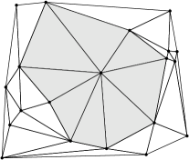
In order to estimate at any general point , one might have used linear interpolation based on the 7 vertices of the corresponding Delaunay cell . This means expressing as a linear function of the 6D vector , namely , with and a 6D vector and a scalar whose seven unknown values are found by equating with at the seven vertices of the cell. However, with particles involving Delaunay cells the linear interpolation is CPU-expensive and practically impossible. Instead, we perform a zero-order interpolation where is constant inside each Delaunay cell – the average of the values at the seven vertices of :
| (28) |
This has the advantage that any integral of the form
| (29) |
with some arbitrary function, can be easily estimated by the sum
| (30) |
In particular, the desired can be found by first computing its cumulative counterpart ,
| (31) | |||||
| (32) |
and then taking its derivative,
| (33) |
In what follows, we often denote the DTFE-measured and by and in order to distinguish them from the exact quantities.
3.3 Error Estimate
When we measure the of a cosmological -body system using the Delaunay tessellation, we should expect two types of errors. First are the errors in the underlying associated with errors in the numerical simulation itself, such as errors due to two-body relaxation effects, force estimation, time integration and so on. A way to estimate these errors is by re-simulating the same system with different codes and with different sets of numerical parameters governing the mass resolution and the force resolution. A systematic testing of this sort will be reported in an associated paper (Arad, Dekel & Stoehr, in preparation). In the current paper, we make a preliminary comparison of several different haloes simulated with different resolutions and with different codes. We find that all the virialized haloes tested recover almost the same shape of .
The second type of errors originate from the fact that we try to estimate a smooth from a finite set of particles using the Delaunay tessellation. Here we may encounter both statistical and systematic errors. Some of these errors would decrease as the number of particles is increased, whereas some are an inherent part of the DTFE independent of the mass resolution. In order to obtain a simple understanding of the nature of the DTFE errors, we first use a simple statistical model based on a Voronoi tessellation, which resembles the DTFE but lends itself more easily to analytical treatment. We then evaluate the DTFE errors empirically by measuring in synthetic systems were the particles represent a known , and compare the results to the error-model predictions. Since this error analysis is somewhat detached from the main focus of this paper, we describe it in detail in Appendix A. Our wisdom regarding the DTFE properties and uncertainties can be summarised in three points as follows:
(i) The measured at each particle is chosen, to a good extent, from a probability distribution of the random variable . In a typical realisation with particles, the width of this distribution is about one decade, defining the range of fluctuation of about . As , the shape of the distribution approaches an asymptotic limit with a finite width of about one quarter of a decade, as deduced from the DTFE of a Poisson distribution. Therefore, also in the infinite limit, the DTFE is expected to produce local fluctuations.
(ii) The measured can be viewed as a convolution of the true and a fixed window function, which is related to the probability distribution [Eq. (46)]:
| (34) |
For distributions where is close to a power-law, the difference between and is negligible over a large range of scales, as demonstrated in Figs. 9 and 10. This is a very useful feature of the DTFE-measured .
(iii) The relative statistical error in is proportional to , and can be approximated by [Eq. (59)]
| (35) |
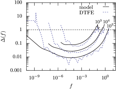
with and . The constant is of order unity, and can be calibrated by comparing Eq. (35) to the actual error in lower-resolution measurements. In practise, this means that when or more, the statistical error in is negligible for a very wide range of . Moreover, in regions where there are large statistical errors, they are likely to be overwhelmed by systematic errors.
4 A UNIVERSAL SCALE-FREE
We have analysed the of several different haloes, in three different mass ranges, simulated within the CDM cosmology with two different -body codes.
In order to calculate the of a given halo, we find the halo centre using a simple max-density algorithm, and extract all particles which lie within a distance from its centre. The max-density algorithm is based on an iterative counting in cells: at each iteration, space is divided into 8 equal cubic cells and the densest cell is chosen for the following iteration. The iterative process stops when the densest cell contains no more than 500 particles, and the centre of that cell is defined as the centre of the halo. The radius is typically set to be larger than the virial radius. We compromise on analysing particles, such that we explore a significant dynamical range while the computation can be completed in a few days.
To estimate the typical phase-space density at the outer regions of the halo, we define by
| (36) |
which is the average space-space density that one would measure for a halo of constant density and a Maxwellian velocity distribution with a velocity dispersion . For a given halo in a given cosmology, the mean virial quantities and are defined using the virial theorem and the top-hat model relevant to that cosmology.
As one crude estimate of the upper limit on for which the measurement of is reliable, we evaluate in each halo the value, , below which the statistical error in due to the DTFE procedure is below . For that we use Eq. (35), calibrated by measurements with particles. This statistical error is expected to be practically negligible in the range .
4.1 -body Simulations on Different Scales
The results described in this paper are based on three different cosmological simulations. Two of them used the Adaptive Refinement Tree (ART) code (Kravtsov, Klypin & Khokhlov, 1997), and the third used the Tree Particle Mesh (TPM) code (Bode et al, 2000; Bode & Ostriker, 2003). In all the simulations, the assumed cosmological model is the standard CDM with , and today.
The ART simulations were done in periodic boxes of sizes and , whereas the TPM simulation was done in a box of . We denote these three simulations by , and respectively. Three haloes were analysed from each of these simulations, with masses corresponding to to dwarf galaxies (), normal galaxies () and clusters () respectively. Global properties of of the simulations and the haloes are given in table 1. The curves for these haloes are shown in Fig. 4.
| Halo | 333units: | 444units: | Code | |||||||||
|---|---|---|---|---|---|---|---|---|---|---|---|---|
| [kpc] | [kpc] | [] | [] | [kpc] | ||||||||
| ART | ||||||||||||
| ART | ||||||||||||
| ART | ||||||||||||
| ART | ||||||||||||
| ART | ||||||||||||
| ART | ||||||||||||
| TPM | ||||||||||||
| TPM | ||||||||||||
| TPM |
The L1 simulation is from Colín et al (2003). It is analysed at in physical coordinates. The three haloes studied, labelled , , , are the largest haloes in the snapshot. Their virial radii refer to a mean overdensity of , as appropriate for the given cosmology and redshift. The L25 simulation is by Klypin et al (2001). The haloes are denoted , , following the notation in the simulation paper. The L320 simulation is by Wambsganss et al (2004); Weller et al (2004). The three haloes studied, labelled , , , are the most massive haloes in the simulation excluding haloes whose real density map shows an ongoing major merger.
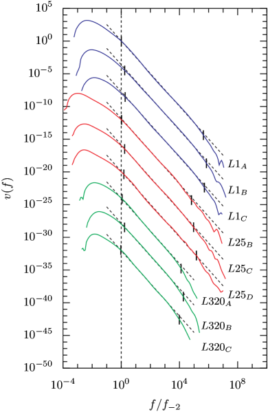
In each of the analysed haloes, we find to be well described by a power-law,
| (37) |
over 3 to 5 decades in . It is typically valid between slightly above and slightly below . Outside this range, gradually and systematically deviates downward from the power law. In the low- regime the deviation is associated with departure from the virial regime, and the high- deviation is consistent with being due to the limited mass resolution of the specific halo, as seen by the proximity to and as demonstrated in Appendix A. The high- deviation from the power-law tends to occur at a smaller value in L25, and even smaller in L320, due to the fact that is smaller respectively.
There is no evidence for a significant dependence of on the halo mass. There may be a marginal trend for slight steepening of as a function of mass, but only from steeper than at to flatter than at . This indicates relative insensitivity to the exact slope of the initial fluctuation power spectrum, which varies across the range from dwarf galaxies to clusters of galaxies. Additionally, the fact that we obtained essentially the same from simulations using two different numerical codes, indicates that the shape of is not an artifact of a particular simulation technique.
5 SUBSTRUCTURES
5.1 Clumpiness in Phase-Space Density
Had been a function of the energy alone, and the haloes were completely spherical and isotropic, the power-law would have implied via Eq. (25) that the real-space density profile must also be a power law, in fact an isothermal sphere , at least over some finite range in . This is clearly not the case, as the simulated haloes are well described by a universal average density profile whose local logarithmic slope is varying continuously from at the outer parts to or even flatter in the inner parts (§1). We conclude that is far from being a function of energy alone, and in particular the system must deviate significantly from spherical symmetry or isotropy. This could be mostly due to the clumpy substructure of the halo, where the surviving subhaloes contribute volume of high phase-space density to , thus making it shallower than expected from a smooth system with an inner density slope flatter than .
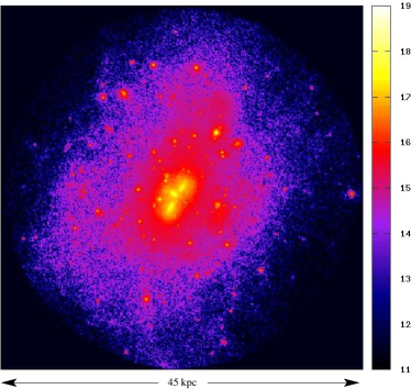
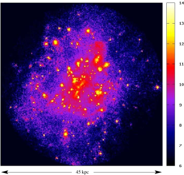
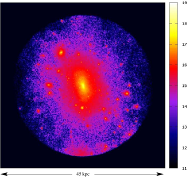
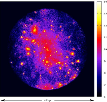
In order to address the hypothesis that is driven by substructure, we plot real-density and phase-space density maps of each halo in real-space slices. Fig. 5 and Fig. 6 show such maps for dwarf haloes B and C (all other haloes show a similar qualitative behaviour).
The real-space density of each particle was calculated using a three-dimensional Voronoi tessellation (van de Weygaert, 1994), generated using the free qhull software package. We chose this technique to estimate the real-space density because it is very similar in its adaptive nature to the Delaunay tessellation technique used to estimate the six-dimensional phase-space density. A brief account of the Voronoi tessellation technique is found in Appendix A, where it is used to estimate the errors in the DTFE method.
The maps were produced in the following way. For each halo, we consider all the particles within an equatorial slice parallel to the -plane, whose width is 40% of the virial radius. The slice is divided into equal cubic cells, with set to have the cells cubic. The density ( or ) assigned to each cell is the average of the densities of all particle within it. ¿From each group of cells with the same and , we plot the one with the highest density.
We see that the real-space density maps are dominated by the familiar relatively smooth trend of density decreasing from the centre outward, with several tight clumps spread throughout the halo. The phase-space density maps, on the other hand, are qualitatively different. While the global trend with radius is much less apparent, the subhaloes become the highest peaks, especially in the outer regions of the halo. For example, the clumps with (yellow-reddish colours) are found everywhere. The very high peaks, with (bright yellow colours), are all found at a considerable distances from the centre. The central peak in is quite modest in comparison; the elongated structures near the centre of dwarf-halo B are most likely subhaloes in the process of merging.
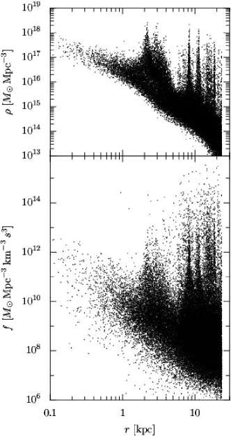
Fig. 7 highlights the same effect by showing and associated with a random subset of the N-body particles as a function of their distance from the halo centre. A large portion of these particles follow the global trend of decreasing density with radius – they could be associated with a smooth-background component, for which is approximately a function of energy alone. At radii , the high- values come in “spikes” corresponding to the subhaloes. While the spikes in reach values comparable to the central peak, the spikes in could be more than 100 times higher, indicating that the subhaloes are both compact and cold. We note in dwarf halo B, for example, that all the points where are in subhaloes.
The other interesting feature of the spikes is the fact that they seem to get lower and broader as they get closer to the halo centre, and that beyond a certain radius (of about ), the spikes completely blend into the smooth background. This indicates that the subhaloes phase-mix and lose their high phase-space densities as they approach the halo centre. This seems to be the natural result of mergers and tidal effects, which both puff up the subhaloes and heat them up.
5.2 Toy Model: Adding Up Small Haloes
As a first attempt at trying to understand how the power law in a halo of mass may originate from its substructure, we simply add up the typical contributions from the general population of haloes of different masses smaller than , as predicted in the CDM cosmology. Based on cosmological N-body simulations (Moore et al, 1999a; Ghigna el al, 2000; De Lucia et al., 2004), and in accordance with the Press-Schechter approximation (Press & Schechter, 1974) and its extensions (e.g., Lacey & Cole, 1993; Sheth, 2003), the mass function of small-mass haloes (not necessarily subhaloes) can be approximated by , with . Additionally, we assume that the average density profiles of haloes of different masses have the same functional form and are simply scaled versions of each other. This is established by -body simulations for the case of isolated haloes, but is less clear when one considers subhaloes (e.g., Hayashi et at, 2003). Nevertheless, we adopt this assumption as our first crude toy model.
As a first approximation we assume that the haloes all form at the same time in an Einstein-deSitter cosmology, so they have the same characteristic real-space density (a constant factor times the universal density), and therefore their typical radii scale like . Based on the virial theorem, the velocity dispersions then scale like . Therefore, the typical phase-space volume of a halo of mass scales like , and its typical phase-space density is . If we denote by the universal, un-scaled, normalised, dimensionless probability distribution function relevant for all the haloes, then the volume distribution function of a halo of mass , defined such that is a volume, is given by
| (38) |
Then the total contribution to of halo from the population of smaller haloes is
| (39) |
where is the mass of the largest subhalo (). Changing variables , we finally get
| (40) |
Thus, is a multiple of a power-law and a monotonically increasing function of ; it therefore has to be shallower than the power law . For , this means that is shallower than , which is significantly shallower than the measured . This idealised toy model does not seem to work.
This calculation can be generalised to the case where haloes of smaller masses form first, as implied from the slope of the initial fluctuation power spectrum . For an Einstein-deSitter cosmology, the formation time scales with such that , with , and is the local power index, , at the relevant effective scale for masses . Then, in analogy to the calculation in the previous paragraph, we have , , , and we finally obtain that must be flatter than the power law
| (41) |
For , namely , the asymptotic index for small haloes where all haloes form at the same epoch, we recover the earlier result that is flatter than . For CDM on galactic scales, the effective power index is , so , and for we obtain that is flatter than . We see that the time dependence makes only a little difference.
The total of the halo should be the sum of the background contribution and the subhalo contribution, but at the high- range we expect to be dominated by the contribution of subhaloes, as seen earlier in this section. The above toy model thus predicts that should be flatter than , in conflict with the measured .
We conclude that a halo is not simply an ensemble of clumps drawn from the general population of smaller haloes. The subhaloes may have a different mass function, their shape properties may vary differently with mass, and they both could vary with distance from the host-halo centre. If one keeps the scaling relation with and ignores any variation with , the required subhalo mass function for matching the measured is with (compared to ). Indeed, a flattening of the subhalo mass function could be a natural result of the inevitable dynamical evolution of the subhaloes in the potential well of their host halo. The phase mixing due to tidal effects, including total disruption, is likely to be more efficient in less massive subhaloes, thus flattening the mass function. Also, dynamical friction is more efficient in making more massive subhaloes sink into the halo, thus making the mass function flatter in the inner parts. However, recent simulations indicate that the subhalo mass function is not flatter than (De Lucia et al., 2004), indicating that the tidal effects on the inner structure of subhaloes must also have an important role. These are matters for more detailed future studies, but the failure of the idealised toy model analysed above to reproduce the magic power law indicates that the phase-space density is likely to provide a useful tool for studying the dynamical evolution of subhaloes in host haloes.
6 DISCUSSION AND CONCLUSION
Using Delaunay tessellation, we developed a method for measuring the 6-dimensional coarse-grained phase-space density in -body systems. We focused, in particular, on measuring the phase-space volume distribution function, . We applied this technique to several simulated haloes of particles, formed by hierarchical clustering in the standard CDM scenario, and obtained two striking new results.
First, is well described by a power law, , over 3 to 5 decades in . The power-law regime starts at an value which corresponds to the characteristic size of the virialized halo. It ends at an value which is determined by the dynamical resolution limit of the specific simulation. Therefore, the true power-law range may extend to . This power law seems to be insensitive to the halo mass in the range , indicating insensitivity to the exact slope of the fluctuation power spectrum, as long as the haloes are built by hierarchical merging of clumps bottom up.
Second, this power-law originates from substructures within the halo rather then the overall trend with radius. The substructure completely dominates the high- parts of the distribution. The infalling clumps seem to phase-mix — by puffing up, heating and stripping — as their orbits decay from the virial radius inwards toward the halo centre and they melt into the halo smooth background.
Our first worry is that these results could be numerical artifacts, or severely contaminated by such. Based on our error analysis and tests with mock datasets, we argue that the measured by the DTFE algorithm genuinely reflects the true phase-space properties of the given -body system over a broad range of . The question is whether the phase mixing suffered by the subclumps as they approach the halo centre might be an artifact of numerical effects such as two-body relaxation, leading to underestimated inner densities and/or overestimated internal velocities. A similar effect has been pointed out using a one-dimensional toy model (Binney, 2003). The apparent agreement between simulations run with different codes and different resolutions is encouraging. In order to specifically address the effect of few-body relaxation, we intend to run twice a simulation of the same halo with the same number of particles but with a different force resolution (ongoing work with F. Stoehr).
Assuming that the simulations genuinely reflect the true physical behaviour under the Vlasov equation, the origin of the robust power-law shape of from the merging substructure becomes a very interesting theoretical issue. As demonstrated in §5, a simple model using the mass function and the scaled profiles of the general halo population in the CDM scenario does not reproduce the correct power law. This, and the apparent trend of the spikes with radius, indicate that the structural and kinematic evolution of the subhaloes in the parent halo are important. Studies of tidal heating and stripping may be found useful in this modelling.
It would be interesting to follow the phase-space evolution and the contribution to the overall by a single, highly resolved subhalo, or many of those, as they orbit within the parent halo and approach its centre. This may help us understand the nature of the interaction between the parent halo and its subhaloes, and the origin of the power law (ongoing works with E. Hayashi and with B. Moore).
Another more general but speculative possibility is that the power law represents some sort of a cascade of relaxation processed in phase-space, in which high phase-space densities turn into lower (coarse-grained) densities through the process of mixing. In general, the fact that our findings are expressed in terms of the fundamental concept of phase-space density should make them more directly accessible to analytical treatment. In this respect, it may prove beneficial to investigate more closely the time evolution of the of a cosmological halo and its components. This may shed light on the connection between the power-law behaviour and the relaxation processes within the halo.
We saw that the power-law behavior of is limited to the virial regime. It would be interesting to learn how this shape evolves in time as the halo virializes. A preliminary study (to be concluded and reported in another paper) indicates that in the intermediate- regime the of a pre-virialized system is significantly flatter than , while in the high- regime it drops in a much steeper way. The behaviour seems to be a feature unique to virialized systems.
We learnt that in the haloes that are built by hierarchical clustering, the power-law behaviour reflects the halo substructure. It would be interesting to find out whether this power-law behaviour actually requires substructure, or it is a more general phenomenon of virialized gravitating systems, valid independently of substructure. One way to answer this question would be to analyse simulated haloes in which all fluctuations of wavelengths smaller than the halo scale were removed, resulting in a smooth halo formed by monolithic collapse, with no apparent substructure in the final configuration. As described in §1, such haloes are known to still have NFW-like density profiles in real space, and one wonders whether they also have the magic power-law . There are preliminary indications for a steeper in this case (Arad, Dekel & Moore, in preparation). If confirmed, it would indicate that the behaviour, while insensitive to the exact slope of the initial power spectrum, is unique to the hierarchical clustering process, and is not a general result of violent relaxation.
Our current results are just first hints from what seems to be a promising rich new tool for analysing the dynamics and structure of virialized gravitating systems. The analysis could become even more interesting when applied to haloes including the associated gaseous and stellar components.
Acknowledgments
We thank Paul Bode for making his earlier simulations available for analysis. We acknowledge related ongoing collaborations with Stefan Gottloeber, Eric Hayashi & Julio Navarro, Ben Moore and Felix Stoehr. We are grateful for stimulating discussions with Stefan Colombi, Donald Lynden-Bell, Gary Mamon, Jerry Ostriker and Simon White. Part of this work has been done at the IAP in Paris. AK acknowledges support of NASA and ASF grants to NMSU. Our simulations were performed at the National Energy Research Scientific Computing Centre (NERSC). IA is a Marie Curie Postdoctoral Fellow. AD is a Miller Visiting Professor at UC Berkeley. This research has been supported by the Israel Science Foundation grant 213/02, by the German-Israel Science Foundation grant I-629-62.14/1999, and by NASA ATP grant NAG5-8218.
References
- (1)
- Alvarez, Shapiro & Martel (2002) Alvarez M.A., Shapiro P.R., Martel H., 2002, AAS, 200, 4103
- Avila-Reese et al. (2001) Avila-Reese V., Colmn P., Valenzuela O., D’Onghia E., Firmani C., 2001, ApJ, 559, 516
- Bernardeau & van de Weygaert (1996) Bernardeau F., van de Weygaert R., 1996, MNRAS, 279, 693
- Binney & Tremaine (1987) Binney, J., Tremaine S., 1987, Galactic Dynamics (Princeton Univ Press)
- Binney (2003) Binney J., 2003, astro-ph/0311155, submitted to MNRAS.
- Bode et al (2000) Bode P., Ostriker J. P., Xu. G., 2000, ApJS, 128, 561
- Bode & Ostriker (2003) Bode P., Ostriker J. P., 2003, ApJS, 141, 1
- Bullock et al. (2001b) Bullock J. S., Dekel A., Kolatt T. S., Kravtsov A. V., Klypin A. A., Porciani C., Primack J. R., 2001b, ApJ, 555, 240
- Bullock et al. (2001a) Bullock J. S., Kolatt T. S., Sigad Y., Somerville R. S., Kravtsov A. V., Klypin A. A., Primack J. R., Dekel A., 2001a, MNRAS, 321, 559
- Bullock, Kravtsov & Colin (2002) Bullock J. S., Kravtsov A. V., Colin P., 2002, ApJL, 564, 1
- Cole & Lacey (1996) Cole S., Lacey C., 1996, MNRAS, 281, 716
- Colín et al (2000a) Colín P., Klypin A., Kravtsov A. V., 2000, ApJ, 539, 561
- Colín et al (2000b) Colín P., Avila-Reese V., Valenzuela O., 2000, ApJ, 542, 622
- Colín et al (2003) Colín P., Klypin A., Valenzuela O., Gottlöber S., 2003, astro-ph/0308348, submitted to ApJ.
- Dalal & Kochanek (2002) Dalal N., Kochanek C. S., (2002), ApJ, 572, 25
- Dekel, Kowitt & Shaham (1981) Dekel A., Kowitt M., Shaham J., 1981, ApJ, 250, 567.
- Dekel, Devor & Hetzroni (2003) Dekel A., Devor J., Hetzroni G., 2003, MNRAS, 341, 326.
- Dekel et al. (2003) Dekel A., Arad I., Devor J., Birnboim Y., 2003, ApJ, 588, 680
- Delaunay (1934) Delaunay B. V., 1934, Bull. Acad. Sci (VII) Classe Sci. Mat., 793
- De Lucia et al. (2004) De Lucia G., Kauffmann G., Springel V., White S. D. M., Lanzoni B., Stoehr F., Tormen G., Yoshida N., 2004, MNRAS, 348, 333
- Fillmore and Goldreich (1984) Fillmore J. A., Goldreich P., 1984, ApJ, 281, 1
- Gunn and Gott (1972) Gunn J. E, Gott J. R., 1972, ApJ, 176, 1
- Ghigna el al (2000) Ghigna S., Moore B., Governato F., Lake G., Quinn T., Stadel J., 2000, ApJ, 544, 616
- Hayashi et at (2003) Hayashi E., Navarro J. F., Taylor J., Stadel J., Quinn T., 2003, ApJ, 584, 541
- Hayashi et al (2004) Hayashi E., Navarro J. F., Power C., Jenkins A., Frenk C. S., White D. M., Springel V., Stadel J., Quinn T. R., MNRAS, submitted (astro-ph/0310576)
- Hocknet & Eastwod (1982) Hockney R. W., Eastwood J. W., 1981, Computer simulations using particles (New York: McGraw-Hill)
- Hoffman & Shaham (1985) Hoffman Y., Shaham J., 1985, ApJ, 297, 16
- Huss et al (1999a) Huss A., Jain B., Steinmetz M., 1999, ApJ, 517, 64
- Huss et al (1999b) Huss A., Jain B., Steinmetz M., 1999, MNRAS, 308, 1011
- Ibata et al (1994) Ibata R., Gilmore G., Irwin M., 1994, Nature, 370, 194
- Ibata et al (2001a) Ibata R., Irwin M., Lewis G. F., Stolte A., 2001, ApJ, 547, 133
- Ibata et al (2001b) Ibata R., Irwin M., Lewis G. F., Ferguson A., Tanvir N., 2001, Nature, 412, 49
- Klypin et al. (1999a) Klypin A., Gottloeber S., Kravtsov A. V., Khokhlov A. M., 1999a, ApJ, 516, 530
- Klypin et al. (1999b) Klypin A., Kravtsov A. V., Valenzuela O., Prada F., 1999b, ApJ, 522, 82
- Klypin et al (2001) Klypin A., Kravtsov A. V., Bullock J. S., Primack J. R., 2001, ApJ, 554, 903
- Kravtsov, Klypin & Khokhlov (1997) Kravtsov A. V., Klypin A., Khokhlov A. M., 1997, ApJS, 111, 73
- Lacey & Cole (1993) Lacey C., Cole S., 1993, MNRAS, 262, 627
- Lynden-Bell (1967) Lynden-Bell D., 1967, MNRAS, 136, 101
- Maller & Dekel (2002) Maller A. H., Dekel A., 2002, MNRAS, 335, 487
- Maller, Dekel & Somerville (2002) Maller A. H., Dekel A., Somerville, R. S., 2002, MNRAS, 329, 423
- Mathur (1988) Mathur S. D., 1988, MNRAS, 231, 367
- Moore et al (1998) Moore B., Governato F., Quinn T., Stadel J., Lake G., 1998, ApJ, 499, L5
- Moore et al (1999a) Moore B., Ghigna S., Governato F., Lake G., Quinn T., Stadel J., Tozzi P., 1999, ApJ, 524, L19
- Moore et al. (1999b) Moore B., Quinn T., Governato F., Stadel J., Lake, G., 1999b, MNRAS, 310, 1147
- Navarro, Frenk & White (1995) Navarro J. F., Frenk C. S., White S. D. M, 1995, MNRAS, 275, 720
- Navarro, Frenk & White (1996) Navarro J. F., Frenk C. S., White S. D. M, 1996, ApJ, 462, 563
- Navarro, Frenk & White (1997) Navarro J. F., Frenk C. S., White S. D. M, 1997, ApJ, 490, 493
- Navarro & Steinmetz (2000) Navarro J. F., Steinmetz M., 2000, ApJ, 538, 477
- Navarro et al (2004) Navarro J. F., Hayashi E., Power C., Jenkins A., Frenk C. S., White S. D. M., Springel V., Stadel J., Quinn T. R., MNRAS, submitted (astro-ph/0311231)
- Nusser & Sheth (1999) Nusser A., Sheth R., 1999, MNRAS, 303, 685
- Power et al (2003) Power C., Navarro J. F., Jenkins A., Frenk C. S., White S. D. M., Springel V., Stadel J., Quinn T. R., MNRAS, 338, 14
- Press & Schechter (1974) Press W. H., Schechter P., 1974, ApJ, 187, 425
- Ricotti (2003) Ricotti M., 2003, MNRAS, 334, 1237
- Schaap & van de Weygaert (2000) Schaap W., van de Weygaert R., 2000, A&A, 363, L29
- Sheth (2003) Sheth R. K., 2003, MNRAS, 345, 2000
- Su & Drysdale (1995) Su P., Drysdale R. L. S., 1995, Proceedings of the eleventh annual symposium on Computational geometry, p 61
- Subramanian, Cen & Ostriker (2000) Subramanian K., Cen R., Ostriker J. P., ApJ, 538, 528
- Syer & White (1998) Syer D., White S. D. M., 1998, MNRAS, 293, 337
- Tanemura, Ogawa & Ogita (1983) Tanemura M., Ogawa T., Ogita N., 1983, Journal of Computational Physics, 51, 191
- Taylor & Navarro (2001) Taylor J. E., Navarro J. F., 2001, ApJ, 563, 483
- Tremaine, Hénon & Lynden-Bell (1986) Tremaine S., Hénon M., Lynden-Bell D., (1986), MNRAS, 219, 285
- van de Weygaert (1994) van de Weygaert R., 2000, A&A, 363, L29.
- Valenzuela & Klypin (2003) Valenzuela O, Klypin A., 2003, MNRAS345, 406
- Wambsganss et al (2004) Wambsganss J., Bode P., Ostriker J. P., sumbitted to ApJ, astro-ph/0306088
- Weinberg & Katz (2002) Weinberg M. D., Katz N., 2002, ApJ, 580, 627
- Weller et al (2004) Weller J., Bode P., Ostriker J. P., in preperation.
- White & Zaritsky (1992) White S. D. M., Zaritsky D., 1992, ApJ, 394, 1
Appendix A ERRORS IN
The “true”, underlying coarse-grained is what one would have measured using a fixed smoothing window in phase space (e.g. counts in fixed cells) and an arbitrarily large number of particles. Instead, the Delaunay Tessellation Field Estimator uses adaptive cells in order to deal with the mass resolution limitations. Therefore, the relation between the measured and the underlying is not trivial. Both statistical and systematic errors might influence our results. We estimate these errors empirically below, but we start with an approximate model that provides a simple understanding of the origin of the errors.
A.1 A Voronoi Model: Fixed Smoothing
A technique similar to the Delaunay tessellation, but somewhat simpler to interpret, is the Voronoi tessellation (van de Weygaert, 1994). For each particle, the Voronoi cell is defined as the region of phase space in which every point is closer to that particle than to any other particle. In this case, particles define exactly Voronoi cells which cover all of phase space with no overlaps. If is the Voronoi cell of particle , then a natural mass-preserving way of estimating the phase-space density inside that cell is by . We denote the quantities measured this way by and .
Much like the Delaunay tessellation, the Voronoi tessellation is an adaptive grid that enables one to estimate even in the presence of a relatively small number of particles. We use the Delaunay method in our main analysis because it is somewhat more accurate (Schaap & van de Weygaert, 2000), and is easier to calculate numerically. However, the similar Voronoi method provides a simple way of learning about the properties of the measured and understanding the uncertainties associated with such a measurement. The empirical tests of the Delaunay measurements below demonstrate the relevance of the wisdom gained by analysing the Voronoi model.
To understand the errors in the Voronoi density estimation, let us start with the trivial case where all of infinite phase-space is uniformly filled with phase-space density , which is represented by an infinite number of particles with mass . A volume of phase-space would then contain on average a finite number of particles, . The Voronoi estimate of for each particle would fluctuate about due to the discreteness of the particle distribution. Since there is no typical scale in the problem, and each cell always contains one particle, the fluctuations per Voronoi cell would remain at the same level even if one increases the average number density of particles while decreasing the mass of each particle in proportion, keeping the same. Therefore, the probability that the Voronoi estimated would lie in the interval may be written in terms of a universal probability distribution function .
When we consider a finite system in a box of volume , with a finite number of particles inside it, we may expect the probability distribution to deviate from its asymptotic form . As decreases, we expect to widen due to the increasing effect of the boundaries. Next, examine a system with a non-uniform phase-space density, such as a cosmological halo. If the number of particles that represent this is sufficiently large, we may approximate every region in phase-space as being locally uniform, and estimate its Voronoi using the asymptotic . This assumption is expected to break down in regions with very high phase-space density, where the sampling may become poor and insufficient, or in regions where has large gradients over small scales. Nevertheless, lets assume for the moment that there exists an effective [not necessarily ] which properly approximates the fluctuation distribution of the Voronoi for all particles.
This assumption allows us to calculate the expectation value of for a finite system with a given . This is done by first calculating the average of , the cumulative version of defined in (9), and then differentiate it to obtain the average of . Assuming that is realised by particles, we divide phase space into a large number of cells , which are small enough to guarantee that (a) each cell is very unlikely to contain more than one of the particles, and (b) the value of is approximately constant within every cell.
For each cell , we calculate , the average of the contribution of this cell to . The contribution would be non-zero only when there is a particle in the cell , a particle whose assigned Voronoi estimated density is . If is the true phase-space density in that the cell, then, according to our assumption, would be chosen at random out of the probability distribution . Once is chosen, is given by
| (42) |
Using our assumption (a) above, the probability of to host one particle is , with the total mass of the system. Therefore,
| (43) | |||||
| (44) |
and so,
| (45) | |||||
In the last equality, we have used the exact to replace the six-dimensional phase-space integration. By differentiating Eq. (45) with respect to , we finally obtain the desired expectation value:
| (46) |
We see that the measured is a convolution of the exact with a fixed window function . The narrower is, the closer would be to the true . However, as argued above, even when the window does not approach a Dirac delta function; it rather converges to some finite-width distribution . Therefore, even with an infinite resolution the Voronoi tessellation would not produce the exact ; it converges to a convolution of it with a fixed window .
This convolution would not affect the shape of the measured , and would preserve the true shape of , provided that does not vary drastically over scales which are smaller than the width of the window. In particular, when is a power law, the Voronoi algorithm would recover the same power law for .
A.2 Empirical Testing with Mock Systems
For an empirical study of the errors in the DTFE-measured , and for testing how well the Voronoi model approximates these errors, we have performed a series of measurements on systems with known phase-space densities of the form
| (47) |
corresponding to a spherical system in real space with a Maxwellian velocity dispersion. We have examined six such systems with three different density profiles parametrised by ,
| (48) |
and the following two types of dispersion profiles:
| (49) | |||||
| (50) |
The subscripts “v” or “c” denote a varying dispersion profile versus a constant one respectively. The for such systems is
| (51) |
with
| (52) |
and its inverse.
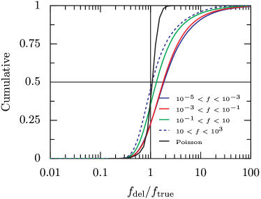
Figure 8 shows the cumulative distributions of in different bins of , for the system and the system. Both systems were realised using particles. In both cases we have also plotted the cumulative distribution for a homogeneous Poisson distribution, realised in a six-dimensional cubic box with particles. We have verified that this distribution is essentially unchanged when the calculation is done with particles. Therefore, it should be regarded as good approximation to the asymptotic limit we would have reached in the different bins, had we used an infinite number of particles. The other four systems give essentially the same results.
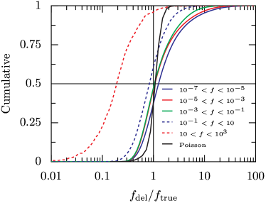
In the 1-v system, five bins were defined by . We see that the shape of the distribution, corresponding to the width of the differential distribution, is very much independent of . For all bins, the full width is less than a 1.5 decades. On the other hand, there does seem to be a systematic shift of the median toward larger values of for smaller values of . The large shift of the highest- bin () toward small is a result of the very low number of particles in that bin, less than 500, which is insufficient for representing such high phase-space densities.
The bias toward larger phase-space densities in the low- bins may be attributed to boundary effects: while the total mass of the particles in the realisation is equal to the total mass one would obtain from the exact integrated over the infinite phase-space, the total phase-space volume used by the DTFE to estimate is finite. It is the smallest possible convex polygon containing all particles. Therefore, we may expect an overestimate of , which would be more pronounced near the boundaries. Nevertheless, as we shall see by comparing to , on scales of a few-decades, this bias is rather meaningless.
The distributions of the 1-c system are essentially the same as the ones in the 1-v system. Here 4 bins were defined by . The overall shape of the plots changes very little from bin to bin, and its width is about a decade and a half. Additionally there exists the bias towards larger ratios as gets smaller.
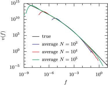
To see how well the DTFE reconstructs the true , we have measured the of the six mock systems using , and particles for each system. Figures 9, 10 present the results of these numerical experiments. We see that with the highest resolution, of particles, the recovery is excellent over a range of almost 7 decades in . Systematic deviations begin at the high- end and the low- end. At both ends, the deviations appear at about one to two decades inward to the highest and lowest values of in that realisation. When the resolution is decreased, the -range where closely matches narrows gradually.
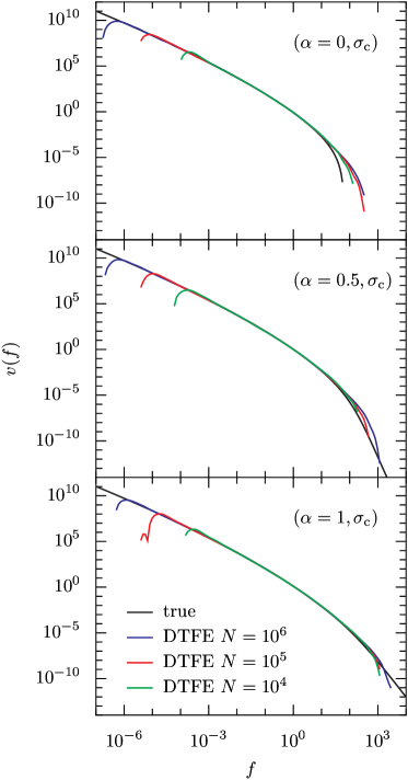
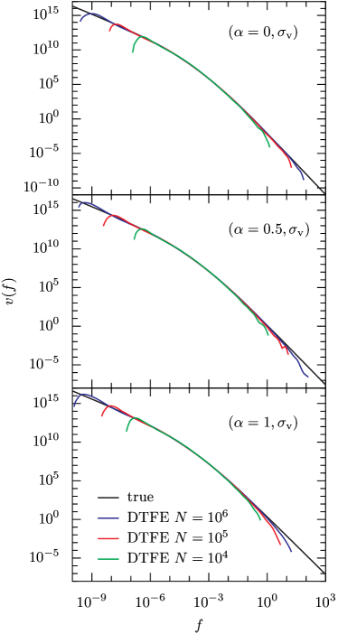
As argued above, the systematic deviations at the low- end are probably a result of the finite phase-space volume occupied by the particles. As the number of particles is increased, a larger portion of phase-space is covered, enabling the reconstruction of lower values of .
The high- systematic deviations can be qualitatively understood using the Voronoi model and its convolution formula (46). Since the DTFE uses a finite number of particles to recover the field, there must be an upper cutoff, , for the spectrum of values that the DTFE can produce in principle. As far as the DTFE is concerned, the true has an effective cutoff at . If we plug this “true” truncated into the convolution formula (46), assume a distribution function with a width of about 1 decade, and set , we recover the qualitative behaviour of the measured for the mock samples with and the three values of . This simple picture is, however, an oversimplification because the high- region is also effected by statistical fluctuations due to the low number of particles there.
The convolution formula can also explain the overestimation by the in the high- regions of the mock systems with . In these systems, the transition between the low- power-law and the steep high- decline is rather sharp; it occurs over a scale comparable to the width of the window function . As a result, the measurement at a high- includes contributions from the higher values at lower . This becomes very apparent in the case with and , in which has an upper bound of . While the true vanishes for all values larger than this limit, the DTFE-measured vanishes only at an value that is an order-of-magnitude larger, due to the 1-decade width of the assumed probability distribution function .
A.3 Statistical Errors in .
The Voronoi model can also be used to estimate the statistical errors in . Strictly speaking, is an ill-defined random variable, as it is measured by differentiating , which is a super-position of Heaviside step functions, and as such is a sum of Dirac delta functions. Much like a white-noise process, its variance is infinite. In practise, however, we always compute by differentiating a smoothed version of (using a spline, for example). Therefore, we may expect the statistical error in to be comparable to the statistical error in . The latter can be estimated in a way similar to how we estimated the average of .
To calculate , we can use the definition of to write
| (53) |
Assuming that is independent of , the cross terms would cancel out from , leaving us with the upper limit
| (54) |
Using arguments similar to those used for calculating , one can show that
| (55) | |||||
| (56) | |||||
| (57) |
Therefore,
| (58) |
and the relative error is given by
| (59) |
Plugging into the formula above, where is the total mass of the system and the total number of particles, we recover the common large-numbers limit .
To check how good this estimate is for the DTFE-measured , we have measured the of 100 realisations of the mock system with and particles, and 30 realisations with particles. From these measurements we computed the true relative error in [with respect to the average of the DTFE-measured , not with respect to the exact ], and compared it to the prediction of Eq. (59). Figure 11 shows the comparison for the three resolutions. We see that Eq. (59) performs well as an upper bound for the statistical errors, except for the low- region. In that region the cumulative approaches a constant as , due to the finite phase-space volume of the halo. This introduces fluctuations to as a result of the numerical differentiation in Eq. (33).
However, it is interesting to notice that whenever the statistical errors in become important, they are overwhelmed by the low- or high- systematic errors. In that respect, the statistical errors in are of no big relevance.
