Detection of X-ray Clusters of Galaxies by Matching RASS Photons and SDSS Galaxies within GAVO

A new method for a simultaneous search for clusters of galaxies in X-ray photon maps and optical galaxy maps is described. The merging of X-ray and optical data improves the source identification so that a large amount of telescope time for spectroscopic follow-up can be saved. The method appears thus ideally suited for the analysis of the recently proposed wide-angle X-ray missions like DUO and ROSITA. As a first application, clusters are extracted from the 3rd version of the ROSAT All-Sky Survey and the Early Date Release of the Sloan Digital Sky Survey (SDSS). The time-consuming computations are performed within the German Astrophysical Virtual Observatory (GAVO). On a test area of 140 square degrees, 75 X-ray clusters are detected down to an X-ray flux limit of $3-5\times 10^{-13}\,{\rm erg}\,{\rm s}^{-1}\,{\rm cm}^{-2}$ in the ROSAT energy band 0.1-2.4 keV. The clusters have redshifts $z\leq 0.5$. The survey thus fills the gap between traditional large-area X-ray surveys and serendipitous X-ray cluster searches based on pointed observations, and has the potential to yield about 4,000 X-ray clusters after completion of SDSS.

1 Introduction

Clusters of galaxies trace the peaks of the matter distribution and their dynamics on cosmic scales (see review in Borgani & Guzzo 2001). The corresponding cluster number density fluctuations can be measured up to Gigaparsec scales where they display a simple Gaussian random field with a high statistical significance (Schuecker et al. 2002, 2003a). Therefore, the related mean spatial abundance, the two-point correlation function, and the power spectrum give a useful summary of these fluctuations. They are well fit by a flat, low density Cold Dark Matter model without any significant contribution of dark energy others than the cosmological constant (Schuecker et al. 2003b). The data further support a simple scale-invariant biasing scheme although the details are still discussed controversal (e.g., Bahcall 1988, Collins et al. 2000, Schuecker et al. 2001, Zandivarez, Abadi & Lambas 2001).

The usuability of rich clusters for cosmological investigations is mainly related to their simple statistical properties and to their comparatively simple physical structure (e.g. Kaiser 1986, Sarazin 1988, Neumann & Arnaud 2001). This is especially the case for X-ray clusters of galaxies where the X-ray flux limit provides a clean measure of the cluster selection function. A crucial point is the reliability of cluster mass estimates (Schindler & Müller 1993, Evrard, Metzler & Navarro 1996) where evolutionary effects could further complicate the tests (Vikhlinin et al. 2002). However, for not too distant systems the effects are found to be small (e.g. Gioia et al. 2001, Rosati, Borgani & Norman 2001) so that a proper calibration with detailed X-ray observations appears to be possible and is already in progress (H. Böhringer et al., in preparation).

Of fundamental importance for every precise cosmological test is the construction of large, homogeneously selected and thus representative samples. Unfortunately, the time-consuming spectroscopic follow-up observations of the cluster candidates selected from X-ray data hampered the construction of X-ray cluster samples with sizes of the order of $10^{3}$ or more (see review in Edge 2003). A similar problem is expected for the recently proposed large-area X-ray missions like DUO and ROSITA. From the construction of the Northern ROSAT All-Sky (NORAS, Böhringer et al. 2000) and ROSAT ESO Flux-Limited X-ray (REFLEX, Böhringer et al. 2003) samples we learned, however, that a careful pre-selection of cluster candidates can lead to high success rates during the spectroscopic follow-up observations and can thus save a large amount of telescope time (see also Böhringer et al. 1998, 2001, Guzzo et al. 1999).

In the following section we give a description of a general likelihood method for the detection of clusters of galaxies (Sect. 2) which allows a simultaneous analysis of multiwavelength data. In Sect. 3 we apply the method to the X-ray photon distributions as given by the 3rd version of the ROSAT All-Sky Survey (RASS-3, Voges et al. 1999). A new source detection in RASS is necessary because it will turn out that – because we combine X-ray data with much deeper optical data – the new method can go significantly deeper compared to the standard analyses of RASS. For the measurement of the source extent, hardness ratio and other important X-ray quantities the Growth Curve Analyses (GCA) method of Böhringer et al. (2000, 2001) is used. In Sect. 4 we apply the same likelihood method to the galaxy distribution as given by the Early Date Release of the Sloan Digital Sky Survey (SDSS, York et al. 2000) using the $r^{\prime}$ band where completeness and sample sizes are highest down to the faintest magnitudes and which serves as a ‘reference’ passband where most methods using SDSS data are first illustrated (future applications will, however, include all five SDSS bands). The similarity of the source detection in X-rays and cluster search in the optical allows a straightforward merging of the two results (Sect. 5).

In a test area of 140 square degrees, 75 clusters are detected down to the nominal flux-limit of $3-5\times 10^{-13}\,{\rm erg}\,{\rm s}^{-1}\,{\rm cm}^{-2}$ in the ROSAT energy band $0.1-2.4$ keV, that is, 5–10 times deeper than REFLEX. The measured parameters of the clusters are described in Sect. 6. Extrapolated to a final SDSS area of 7,000 square degrees, our method is thus expected to yield about 4,000 X-ray clusters. To test the reliability of our method, we compare in Sect. 7 our X-ray cluster sample with various SDSS and RASS-based catalogues. Further tests with realistic simulations are postponed to a second paper.

It will be seen that a detailed analysis of the RASS and SDSS data requires massive computing power. Moreover, our method allows the inclusion of further high-resolution maps from, e.g., temperature anisotropies of the cosmic microwave background radiation, centimeter or millimeter (Sunyaev-Zel’dovich) maps etc. The combined analysis of such large databases is a typical example where virtual observatories can help with a fast and easy data handling and a distribution of the time-consuming computations over many computer systems (grid computing). The present investigation was thus planned already from its beginning to be performed within the German Astrophysical Virtual Observatory (GAVO).

All computations assume a pressureless Friedmann-Lemaître world model with the Hubble constant $H_{0}$ in units of $h=H_{0}/(100\,{\rm km}\,{\rm s}^{-1}\,{\rm Mpc}^{-1})$, the normalized cosmological constant $\Omega_{\Lambda}=0.73$, and the density parameter $\Omega_{m}=0.27$, but the resulting cluster catalogues do not depend on the chosen values of the cosmic energy densities.

2 A general method for cluster detection

In the following we want to define likelihood functions appropriate for the detection of clusters in point patterns. For the analysis a quantity $L_{V}(\@vec{x}_{1},$ $\ldots,\@vec{x}_{N})$ $d\@vec{x}_{1}\cdots d\@vec{x}_{N}$ is defined which gives the probability of finding exactly one point in each of the infinitesimal volume elements $d\@vec{x}_{1},\ldots,d\@vec{x}_{N}$ centered at $\@vec{x}_{1},\ldots,\@vec{x}_{N}$. We assume that this probability is Poissonian with the intensity parameter $\lambda$. The presence of a cluster suggests that $\lambda$ is closely related to the projected cluster profile (plus background) and is thus a function of $\@vec{x}$. The probability to find a point in a given volume element is thus guided by $\lambda(\@vec{x})$, and is independent of the probability to find somewhere else another point. Because of this independence property, $L_{V}$ is simply the product of $N$ terms, each of the form $\lambda(\@vec{x}_{i})d\@vec{x}_{i}$.

However, the test for the presence of a cluster is still incomplete because we did not include the fact that no further points were observed outside the $N$ infinitesimal volume elements. This probability is given by the void probability function $\exp(-\int\lambda(\@vec{x})d\@vec{x})$ where the integration extends over the volume $V$ reduced by the sum of the infinitesimal volume elements, $d\@vec{x}_{i}$, which can be neglected due to their small size so that, in total, the integration extends over the complete volume $V$. Therefore, an appropriate likelihood function for cluster search is of the form

$$\ln L_{V}\,=\,-\int_{V}\lambda(\@vec{x})d\@vec{x}\,+\,\sum_{i=1}^{N}\,\ln\lambda(\@vec{x}_{i})\,,$$ (1)

which assumes high values when the model distribution $\lambda(\@vec{x})$ fits the observed pattern of $N$ points. Often, additional properties of each point, like its magnitude, colour or energy are available. This information can be directly incorporated, extending the dimensionality of (1) by a further space which includes the additional marks $m$,

$$\ln L_{V\times M}\, = \,-\int_{V}\int_{M}\,\lambda(\@vec{x},m)dm\,d\@vec{x}\,+\,\sum_{i=1}^{N}\,\ln\lambda(\@vec{x}_{i},m_{i})\,.$$

A mathematical exact derivation of (2) is given in Schuecker & Böhringer (1998) where the correctness of this model was verified with a large number of Monte-Carlo experiments. Such additional tests are necessary because sometimes likelihood estimates can yield biased results. Different versions of this matched filter can be found in e.g. Postman et al. (1996), Kepner et al. (1999), Kim et al. (2002). The corresponding detection probability is

$$P\,\equiv\,\frac{L-L_{0}}{L}\,=\,1\,-\,\exp{\left(-\ln\frac{L}{L_{0}}\right)}\,,$$ (3)

with the likelihood ratio $L/L_{0}$ giving a measure of the probability for the presence of a cluster normalized to the probability for the absence of a cluster (blank field). In the following sections we will specialize Eq. (1) to the analysis of the spatial distribution of RASS photons, and Eq. (2) to the analysis of the spatial and magnitude distributions of SDSS galaxies. The likelihood for a cluster present in both X-rays and optical is then simply given by the point-wise product of the two likelihood maps.

3 Cluster detection in RASS-3

For the cluster detection in RASS-3 we assume $\lambda$ to be proportional to the local countrate $c(\@vec{\theta})$, giving the number of X-ray photon events observed in a unit time interval in a specific energy band per arcsec² at the angular coordinate $\@vec{\theta}$ measured (in arcsec) from the centre of the region to be tested for the presence of a cluster. If $t(\@vec{\theta})$ is the exposure time (in seconds) of RASS-3 at $\@vec{\theta}$ then Eq. (1) translates into

$$\ln L\,=\,-\int_{0}^{\infty}d^{2}\@vec{\theta}\,c(\@vec{\theta})\,t(\@vec{\theta})\,+\,\sum_{i=1}^{N}\,\ln\left[c(\@vec{\theta_{i}})\,t(\@vec{\theta_{i}})\right]\,.$$ (4)

For the local countrate we assume the model $c(\@vec{\theta})=\bar{c}+\Lambda\,\tilde{P}(\@vec{\theta}/\theta_{c})$: a local background countrate $\bar{c}$ plus a cluster with the (convolved) apparent cluster profile $\tilde{P}(\@vec{\theta}/\theta_{c})$ and the projected core radius $\theta_{\rm c}$. With the normalization

$$\int_{0}^{\infty}\,d^{2}\@vec{\theta}\,\tilde{P}(\@vec{\theta}/\theta_{c})\,=\,1\,,$$ (5)

and the definition of an effective exposure time

$$t_{\rm eff}\,=\,\int_{0}^{\infty}\,d^{2}\@vec{\theta}\,\tilde{P}(\@vec{\theta}/\theta_{c})\,t(\@vec{\theta})\,,$$ (6)

we get the likelihood for a cluster X-ray source in units of the likelihood for the local background without any source,

$$\ln\left(\frac{L}{L_{0}}\right)\,=\,-\int_{0}^{\infty}d^{2}\@vec{\theta}\,\Lambda\,\tilde{P}(\@vec{\theta}/\theta_{c})\,t(\@vec{\theta})\,+$$

$$\sum_{i=1}^{N}\ln\frac{\bar{c}\,+\,\Lambda\,\tilde{P}(\@vec{\theta}_{i}/\theta_{c})}{\bar{c}}\,,$$ (7)

where $L_{0}$ is given by (4) for $\Lambda=0$. From (3) and the maximization condition $\partial\ln(L/L_{0})/\partial\Lambda=0$ the following two equations are obtained,

$$t_{\rm eff}\,=\,\sum_{i=1}^{N}\frac{\tilde{P}(\@vec{\theta}_{i}/\theta_{c})}{\bar{c}+\Lambda\,\tilde{P}(\@vec{\theta}_{i}/\theta_{c})}\,,$$ (8)

$$\ln\left(\frac{L}{L_{0}}\right)\,=\,-\Lambda\,t_{\rm eff}\,+\,\sum_{i=1}^{N}\ln\frac{\bar{c}+\Lambda\,\tilde{P}(\@vec{\theta}_{i}/\theta_{c})}{\bar{c}}\,,$$ (9)

which are used for cluster detection and countrate determination in the following manner: For a chosen Right Ascension, Declination and redshift, the cluster profile in form of a standard $\beta$ profile (Cavaliere & Fusco-Femiano 1976) with the core radius $r_{c}$ and the slope parameter $\beta$ is transformed from metric to angular scales $\theta_{c}$ and convolved with the average RASS-3 pointspread function of the X-ray energy band to give $\tilde{P}(\@vec{\theta}/\theta_{c})$. The exposure times $t(\@vec{\theta})$ are computed for each position covered by RASS-3 and yield the effective exposure time from Eq. (6), the countrate from (8), and thus the likelihood ratio from (9). The filter is shifted over the three-dimensional survey volume so that sky coordinates, redshifts and countrates which simultaneously maximize Eq. (9) indicate the presence of an X-ray cluster with the detection probability (Eq. 3).

      

Figure 1: X-ray $\beta$ profile of galaxy clusters with the slope parameter $\beta=2/3$, the core radius $150\,h^{-1}\,{\rm kpc}$ at different redshifts, convolved with the point spread functions of RASS-3 for the energy $1.25$ keV and normalized according to Eq. 5. The RASS-3 point spread function closely resembles the curve labeled $z=1.00$.

Figure 2: Maximum likelihood contours ($1\sigma$, $2\sigma$ …) for RASS-3 in the energy range 0.5-2.0 keV. Crosses mark objects found in the merged ROSAT Bright and Faint (RBF) Source Catalogues. Bright X-ray sources at $({\rm R.A.}=20.7^{\circ},{\rm DEC}=-0.70^{\circ})$, $({\rm R.A.}=33.65^{\circ},{\rm DEC}=-0.775^{\circ})$, $({\rm R.A.}=40.675^{\circ},{\rm DEC}=-0.025^{\circ})$ and $({\rm R.A.}=54.20^{\circ},{\rm DEC}=0.60^{\circ})$ have been removed from the RASS-3 photon maps. Note that RBF sources are also shown slightly outside of the SDSS Declination range $[-1.25,+1.25]$ degrees.

Figure 3: Maximum likelihood contours based on RASS-3 X-ray photons (1st and 4th panels, $1\sigma$, $2\sigma$ … contours), SDSS galaxies (2nd and 5th panels, $\geq 10\sigma$) and the combined maximum likelihood contours of RASS-3 and SDSS data (3rd and 6th panels, $\geq 10\sigma$). Crosses mark the position of the deepest X-ray cluster samples available sofar (REFLEX-2, X-ray flux limit $1.8\times 10^{-12}\,{\rm erg}\,{\rm s}^{-1}\,{\rm cm}^{-2}$). Squares mark the position of the X-ray clusters of the final sample. The structure at ${\rm R.A.}=30$ deg and ${\rm DEC}=+0.5$ deg has a too low likelihood in the SDSS galaxy distribution and is thus not included in the final catalogue.

Figure 4: Maximum likelihood contours. Symbols as in Fig. 3. Squares mark the position of the X-ray clusters of the final sample.

Distant and/or compact X-ray clusters might appear point-like in RASS-3. For such sources the countrates converge to quite stable values when the cluster filter slides towards higher redshifts. The same is true for real point-like X-ray sources. Therefore, the cluster-finder described above can also be used for the detection of point sources which can be identified by their high value of the estimated redshift (usually the maximum $z$ of the tested redshift range).

Another important quantity is the number of source counts, i.e., the number of X-ray photons above the X-ray background:

$$N_{\rm ph}\,=\,\Lambda\,t_{\rm eff}\,.$$ (10)

The number of source photons gives a further handle to evaluate the significance of the detected X-ray source and the expected errors of X-ray countrate and fluxes plus an additional error of the background.

3.1 Application to RASS-3

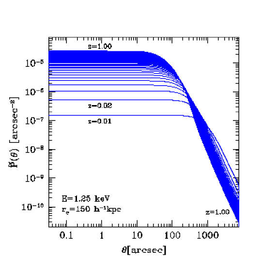
For the cluster detection on RASS-3 we choose a test area of 140 square degrees with $0.0\leq{\rm R.A.}\leq 56$ deg and $-1.25\leq{\rm DEC.}\leq+1.25$ deg (part of the SDSS Early Data Release). Our analysis is restricted to the ROSAT energy range 0.5-2.0 keV where the contrast between X-ray background and cluster is highest (Böhringer et al. 2000). GAVO provides one photon event file and one exposure map of the complete sky based on RASS-3. In the test area and the selected energy band we extracted 180,466 X-ray photons. The median exposure time is 369 seconds which is close to the median exposure time of 388 seconds of the total RASS-3. We assume a standard $\beta$ profile with a fixed shape parameter of $\beta=2/3$ and a fixed core radius of $r_{\rm c}=150\,h^{-1}$ kpc. The profiles are convolved with the spatially averaged point spread function of RASS-3 at 1.25 keV (Boese 2000). A sample of normalized cluster X-ray profiles (see Eq. 5) is plotted in Fig. 1.

For the matched filter only the photons located in a quadratic detection cell with a total area of 1.0 square degree are used (typically 1,200 photons in the energy band 0.5-2.0 keV). This detection cell is shifted by increments of 1.5 arcmin along R.A. and DEC. over the test area. The size of the increment is comparable to the half power radius (96 arcsec) of the point spread function of RASS-3 at 1 keV. In redshift direction the increment is $\Delta z=0.02$ in the range $0.02\leq z\leq 1.0$, consistent with the error estimates obtained with the optical data (Sect. 5). Future investigations will have more computing power and will decrease the increment sizes in all three directions significantly. The local background countrate is estimated with formal Poisson errors $<3$% by the median of the exposure-weighted countrates obtained in a large number of subcells per detection cell. Small background errors are of fundamental importance for the detection of very faint X-ray sources.

The comparatively large size of the detection cell yields stable background estimates. However, bright point sources with countrates of more than about $0.5\,{\rm s}^{-1}$ affect the source detection and background determination significantly. They are detected in a first run of the matched filter and then removed from the RASS-3 photon event file. In the present case we deleted the photons of on average one bright point source per 40 square degrees. After their removal, an almost unbiased search for faint sources can be performed in a second run (see Figs. 2-4).

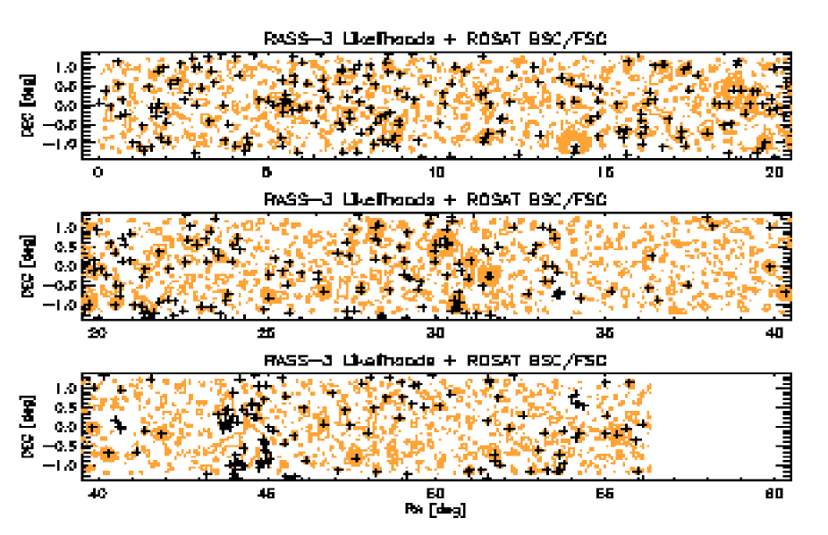
Figure 2 compares the likelihood contours as obtained with the matched filter and the source positions as published in the combined ROSAT Bright and Faint (RBF, Voges et al. 1999) Source Catalogues (crosses). The redshift direction is supressed by replacing the likelihood values obtained along the $z$ direction by their maximum $\ln(L/L_{0})$ value. The latter likelihood together with the R.A. and DEC. are shown. Not shown is the redshift where the maximum likelihood is obtained and the corresponding countrate. In the following we will call these two-dimensional $\ln(L/L_{0})$ arrays maximum likelihood maps. The maximum likelihood contours start at $\ln(L/L_{0})=1.0$ which corresponds to a detection probability of $P=0.63$, i.e., at the $\sim 1\sigma$ detection limit of RASS-3.

A detailed comparison of the results in Sect. 7 shows that the matched filter finds more X-ray clusters than published in RBF. This is due to the fact that the matched filter uses both the RASS and the SDSS data which helps to go below the usual detection threshold of the RBF. We also have a preliminary MPE-internal list of RASS-3 sources obtained with the same detection methods as used for the extraction of the RBF sources on RASS-2, but without a detailed visual screening of the detections. The quantitative comparison in Sect. 7 includes this preliminary source list.

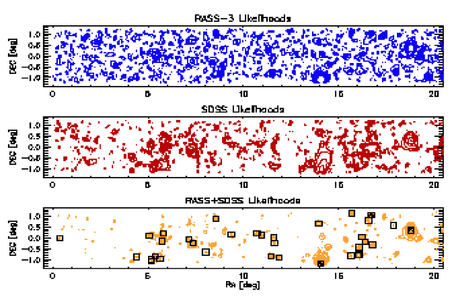
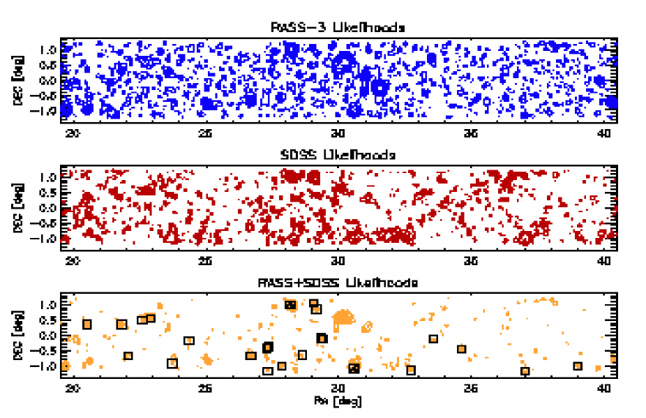
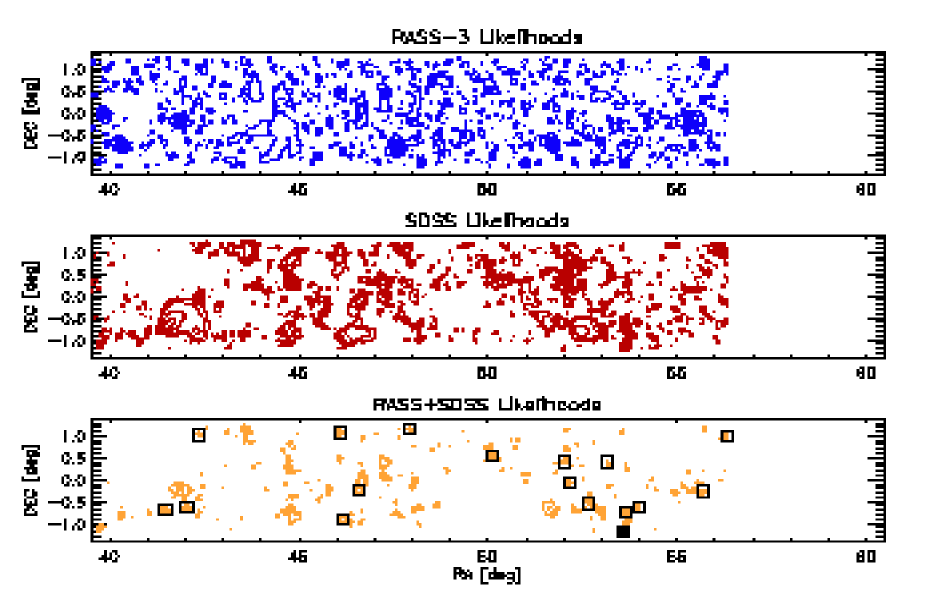
Figures 3 and 4 show (again) the maximum likelihood contours obtained with the RASS-3 survey in the test area, but now in comparison to maximum likelihood maps obtained with the SDSS data and maximum likelihood maps obtained from the combination of RASS and SDSS data. The determination of the SDSS maximum likelihood maps is described in Sect. 4, the combination of RASS and SDSS maximum likelihood maps and preparation of the final cluster sample in Sect. 5. REFLEX-2 clusters and the X-ray clusters of our final RASS/SDSS sample are shown as crosses and squares, respectively, on the combined maps. The REFLEX-2 clusters are clearly visible as the most significant clusters and illustrate that the present method reaches much deeper X-ray flux limits compared to existing RASS-based cluster catalogues.

4 Cluster detection in SDSS

The detection of clusters in SDSS is based on Eq. (2). Our analytic treatment follows Sect. 3 and is described in detail in Schuecker & Böhringer (1998). The final equations are

$$1\,=\,\sum_{i=1}^{N}\frac{P(\@vec{\theta}_{i}/\theta_{c})\,\phi(m_{i}-m^{*})}{\bar{c}+\Lambda\,P(\@vec{\theta}_{i}/\theta_{c})\,\phi(m_{i}-m^{*})}\,,$$ (11)

$$\ln\left(\frac{L}{L_{0}}\right)=-\Lambda+\sum_{i=1}^{N}\ln\left[1+\frac{\Lambda\,P(\@vec{\theta}_{i}/\theta_{c})\,\phi(m_{i}-m^{*})}{b(m_{i})}\right]\,,$$ (12)

which correspond to the Eqs. (8,9) derived for the X-ray data. In Eqs. (11, 12), $\Lambda$ is now the optical richness which is corrected as described in Schuecker & Böhringer (1998), $b(m)$ the average number counts of ‘background’ galaxies with apparent magnitude $m$, $P(\cdot)$ a King-like profile, and $\phi(\cdot)$ the apparent Schechter luminosity function with characteristic apparent magnitude $m^{*}$. Compared to the optical richness, we regard the X-ray luminosity as more directly related to the total gravitating cluster mass (see, e.g., Borgani & Guzzo 2001). Therefore, in the following we do not much concentrate on a discussion of the optical richnesses.

4.1 Application to SDSS

For the optical cluster search, SDSS galaxies with extinction-corrected model magnitudes $r^{\prime}\leq 21.0$ mag are used. Above this magnitude limit a robust star/galaxy separation is expected (Scranton et al. 2003). In our test area we have 2,086,654 SDSS galaxies. A detailed description of our galaxy selection, especially the choice of SDSS catalogue flags, is given in Sect. 4 of Popesso et al. (2003).

For the optical cluster search a truncated King profile with a core radius of $150\,h^{-1}$ kpc and a cutoff radius of $1\,h^{-1}$ Mpc is used. The magnitude distribution of the background galaxies is obtained in detection cells with an area of $5.0\times 2.5$ square degrees (about 180,000 galaxies per detection cell). Although this area might be regarded as comparatively large for the determination of the local galaxy background, we prefer to work with a larger detection area because the RASS-3 clusters are mainly at comparatively small redshifts around $z\approx 0.15$ (Sect. 7) where a good measurement of the bright end of the galaxy luminosity function is needed. A larger area is also better for the detection of nearby less rich systems (Sect. 7).

For the cluster luminosity function we assume a Schechter function with the characteristic magnitude $M^{*}_{r^{\prime}}=-21.43+5\log h$ and the faint end slope of $\alpha=-0.90$ as obtained from the composite luminosity function of SDSS clusters (Goto et al. 2002b). For the conversion of absolute into apparent magnitudes we assumed the $K$-corrections for the early-type galaxies as given in Fukugita, Shimasaku & Ichikawa (1995). The richness estimates are obtained 3.0 mag below the apparent Schechter characteristic magnitude.

In order to allow a direct combination of the likelihood contours, the values of the increment parameters in Right Ascension, Declination, and redshift used for the analysis of the SDSS data are the same as for the X-ray data. The maximum likelihood contours are shown in Figs. 3-4.

5 Combined cluster detection in RASS-3 and SDSS

The similarity of the likelihood filters applied in X-rays and the optical, and the identical sampling of the three-dimensional likelihood parameter space (R.A., DEC., $z$) makes the combination of the results obtained with both data sets by point-wise multiplication of the likelihood values in principle straightforward. However, it turned out that the cluster redshift estimates obtained from the SDSS data are much better compared to the estimates obtained from the RASS data (see Tabs. 2-3). This is mainly caused by the limited angular resolution of RASS. Therefore, we define the final angular coordinates R.A. and DEC. of a cluster by the location of a peak in the multiplied RASS and SDSS maximum likelihood map (Figs. 3-4). The redshift of a cluster is defined by the location of a peak along the $z$ direction in the likelihood map of the SDSS data at the final (R.A.,DEC.) coordinates.

The naive multiplication of maximum likelihood maps from X-ray and optical data and the subsequent peak analyses in the combined map can lead to the detection of spurious X-ray clusters when a strong signal from one energy band is combined with a spurious signal from the other band. The resulting systematics can be reduced by analysing only those peaks in the combined likelihood maps where the related peaks in the X-ray and in the optical maps exceed certain likelihood thresholds.

           

Figure 5: Cumulative X-ray cluster number counts of the RASS/SDSS clusters (histograms) for a log-likelihood minimum of 15 applied to the SDSS data (continuous line), for 25 (lower dashed line), and for 5 (upper dashed line). The RASS/SDSS cluster counts are compared with results obtained with other surveys (points with $1\sigma$ error bars: with RDCS from Rosati et al. 1998 converted to the ROSAT energy band 0.1–2.4 keV assuming a Raymond-Smith spectrum with $z=0$, $k_{\rm B}T=5$ keV, and solar abundance, with REFLEX, and REFLEX-2). No corrections for variations of the angular survey sensitivity (effective survey area) are applied to the RASS/SDSS and REFLEX-2 data (see main text).

           

Figure 6: Fraction of sources with minimum source counts $N_{\rm ph}$ as obtained with the matched filter for the final X-ray cluster sample derive in Sect. 5.

           

Figure 7: Comparison of countrates obtained with the matched filter $\Lambda$ and with the growth curve analysis ctr(GCA) for the final X-ray cluster sample. Not shown are clusters partially outside the test area (1 cluster) and clusters where GCA could not find a clear flattening of the background-subtracted countrates beyond the so-called outer significance radius (6 clusters).

           

Figure 8: Comparison of countrates obtained from RASS-3 with countrates as given in the 2nd ROSAT Source Catalog of Pointed Observations with the Position Sensitive Proportional Counter. The comparison includes all types of X-ray sources.

     

Figure 9: Comparison of cluster redshifts estimated from the SDSS data with spectroscopic cluster redshifts (see Tabs. 2-3).

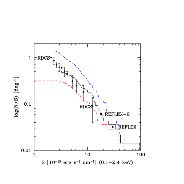
The minimum likelihood threshold for the X-ray data is determined by our goal to search for X-ray clusters down to the detection limit of RASS. In the present investigation we thus use a minimum likelihood of $\ln(L/L_{0})=3.0$ for RASS-3 which corresponds to a detection probability of $P=0.95$. The resulting error rate in RASS is compensated by the high minimum likelihood threshold for SDSS of $\ln(L/L_{0})=15$. This value is found to approximately reproduce the detection of all known comparatively bright REFLEX clusters and limits the number of spurious detections as shown by the flux/number counts in Fig. 5. The determination of cluster X-ray fluxes and related quantities is described in Sect. 6. For this preliminary calibration of the likelihood threshold the RDCS sample was not included because the counts have comparatively large statistical errors in this range. We show the raw RASS/SDSS cluster counts uncorrected for the effective survey area in order to illustrate more directly the results of the cluster search. The final calibration will be performed over a much larger sky area including a proper weighting with the effective survey area.

Tab. 1. Comparison of countrates $\Lambda$ obtained from RASS-3 and as given in the 2RXP catalogue. Col. 1: Minimum countrate (RASS-3). Col. 2: Number of X-ray sources. Col. 3: Average difference $({\rm ctr(RASS3)}$ minus ${\rm ctr(2RXP)})$. Col. 4: Standard deviation of the countrate differences. See also Fig. 8.

$\Lambda>$	$N$	$\Delta(\Lambda)$	$\sigma_{\Lambda}$
$0.100$	$5$	$-0.0039$	$0.0515$
$0.080$	$8$	$-0.0197$	$0.0593$
$0.060$	$13$	$-0.0084$	$0.0558$
$0.040$	$21$	$-0.0037$	$0.0445$
$0.020$	$32$	$+0.0028$	$0.0378$
$0.010$	$50$	$+0.0028$	$0.0306$
$0.008$	$52$	$+0.0024$	$0.0302$
$0.006$	$55$	$+0.0020$	$0.0294$
$0.004$	$61$	$+0.0016$	$0.0280$
$0.002$	$65$	$+0.0012$	$0.0271$
$0.001$	$66$	$+0.0011$	$0.0269$

6 Cluster characteristics

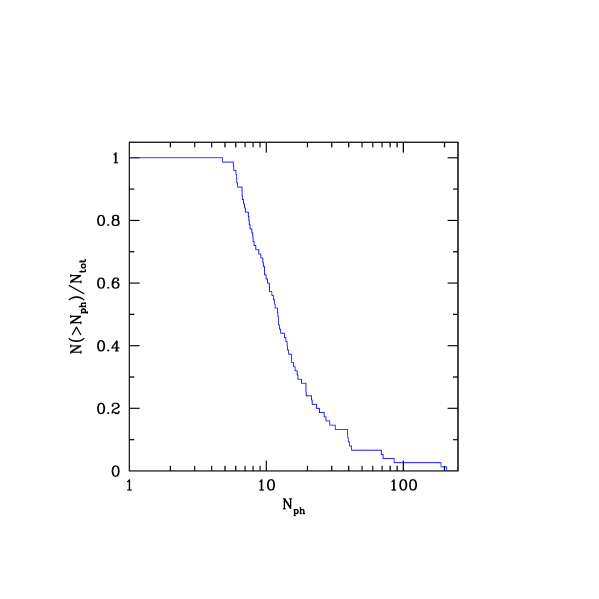
In our test area, 75 clusters fulfill the criteria derived in Sect. 5 (see Tabs. 2-3, squares in Figs. 3-4). Their positions, source counts, effective exposure times, countrates etc. are fixed by their values at the local maxima in the combined maximum likelihood distributions. The X-ray source counts $N_{\rm ph}$ are then determined with Eq. (10). The distribution function of the number of source counts $N_{\rm ph}$ obtained with the final X-ray cluster sample (see Sect. 5) is shown in Fig. 6. The cumulative distribution shows that about 2/3 of the X-ray clusters have at least 10 X-ray photons in the energy range 0.5-2.0 keV above the local background yielding formal errors of the countrates of about 30% (plus negligible errors of $<3\%$ from the background).

Fig. 7 compares the countrates obtained with the matched filter $\Lambda$ and with GCA for our final cluster sample. For countrates $\Lambda>0.05$/s, no significant differences between $\Lambda$ and GCA countrates are seen. For $\Lambda<0.05\,{\rm s}^{-1}$, the matched filter gives on average 15% higher countrates compared to GCA. We attribute this systematic to the fact that the matched filter integrates the source photons out to the edge of the detection cell (formally the integration extends to infinity) whereas the GCA integrates the source photons out to the so-called outer significance radius of a source. Therefore, the former method has the danger of slightly overestimating the countrate, while the latter method does not count the outer wings of the sources and thus slightly underestimates the countrate. The differences between these two integration schemes increase with decreasing countrate as seen in Fig. 7.

GCA further gives for each cluster an additional estimate of the missing flux in order to transform aperature to total X-ray countrates. For example, at a flux of $3\times 10^{-12}\,{\rm erg}\,{\rm s}^{-1}\,{\rm cm}^{-1}$ the average of the latter correction is about 10%. For the matched filter numerical simulations are in preparation to measure the appropriate corrections.

                                                                             

Figure 10: RS17 at $z=0.1092$ with the X-ray flux $S=1.4\times 10^{-12}\,{\rm erg}\,{\rm s}^{-1}\,{\rm cm}^{-2}$ in the ROSAT energy range 0.1-2.4 keV. RS28 at $z=0.2745$ with $S=1.3\times 10^{-12}\,{\rm erg}\,{\rm s}^{-1}\,{\rm cm}^{-2}$.

                                                                             

                                                                             

Figure 11: RS7 at $z=0.0581$ with the X-ray flux $S=5.4\times 10^{-13}\,{\rm erg}\,{\rm s}^{-1}\,{\rm cm}^{-2}$ in the ROSAT energy range 0.1-2.4 keV. The cluster is not in the Bahcall et al (2003) sample. RS26 at $z=0.0663$ with $S=5.1\times 10^{-13}\,{\rm erg}\,{\rm s}^{-1}\,{\rm cm}^{-2}$ is not in the Bahcall et al. (2003) and Goto et al. (2002a) catalogues. RS53 at $z=0.0425$ with $S=3.7\times 10^{-12}\,{\rm erg}\,{\rm s}^{-1}\,{\rm cm}^{-2}$ is not in the Bahcall et al. and Goto et al. catalogues. RS75 at $z=0.1822$ with $S=1.3\times 10^{-12}\,{\rm erg}\,{\rm s}^{-1}\,{\rm cm}^{-2}$ is not in the Bahcall et al. and Goto et al. catalogues. The cluster is also not in the RBF sample extracted from RASS-2 (Voges et al. 1999).

In order to get more information about the reliability of the matched filter countrates, we also compare with the countrates obtained from ROSAT PSPC pointed observations as published in the 2nd ROSAT Source Catalog of Pointed Observations with the Position Sensitive Proportional Counter (2RXP, Fig. 8), independent whether the target is an X-ray cluster or another X-ray source. The comparison is not unrealistic because the majority (80%, see below) of the detected faint X-ray clusters appear point-like in RASS-3a. Averaged systematic and random errors of the countrates obtained with RASS-3 and ROSAT PSPC pointed observations are shown in Table 1. We define a characteristic lower $\Lambda$ limit by the value where the error of the countrate has the same size as the countrate itself. In this case, the comparison suggests a lower limit of about $\Lambda=0.04\,{\rm s}^{-1}$.

Similarily, the systematic errors of the $\Lambda$ countrates as estimated from the comparison with pointed observations range from an underestimation of the countrates of $\sigma_{\Lambda}/\Lambda=3.9$ % for $\Lambda>0.1\,{\rm s}^{-1}$ to an underestimation of 9.3 % at $\Lambda>0.04\,{\rm s}^{-1}$. Below this countrate limit the comparison suggests a possible overestimation of the countrates. One could attribute this error to non-negligible contributions by neighbouring X-ray sources. However, the systematics are of the order of only 10% compared to the random errors at these very low countrates so that one should not overestimate the significance of this effect.

After the countrate/flux conversion of the cluster candidates (see below) we obtain the cumulative flux-number count histogram shown as the continuous line in Fig. 5. Only the raw counts uncorrected for the effective survey area are shown so that the output of the cluster search is seen more directly. The comparison shows that our survey fills the gap between traditional large-area surveys like REFLEX and faint serendipitous surveys like the RDCS (Rosati et al. 1998) which have comparatively large statistical errors in this range. A lower limit of the flux limit can be obtained from the location where the histogram significantly flattens towards faint fluxes (almost independent of the threshold likelihood of the SDSS data). We estimated a nominal flux limit of $3-5\times 10^{-13}\,{\rm erg}\,{\rm s}^{-1}\,{\rm cm}^{2}$ (0.1-2.4 keV). Below this flux limit a strong incompleteness is expected caused by, e.g., surface brightness. A more quantitative analysis needs a larger test area as provided by the SDSS Data Release 2 (coming soon) and a more detailed work on simulated data (P. Schuecker et al., in preparation).

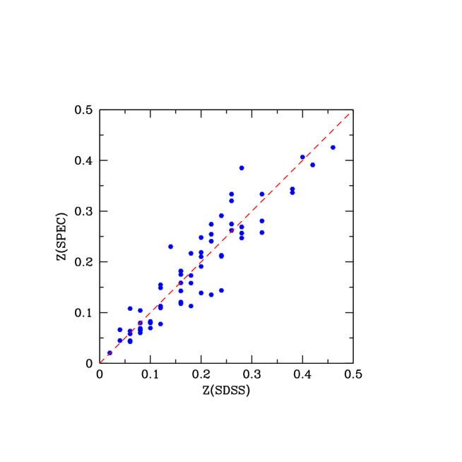
The comparison of the $z$ estimates obtained with the optical data with spectroscopic redshifts shows no significant systematic deviations and underlines the quality of our maximum likelihood cluster redshift estimates (see Fig. 9 and Table 2). Note that X-ray clusters up to redshifts of at least $z=0.5$ can be detected with our method with average redshift errors of about $\sigma_{z}=0.03$.

Tables 2 and 3 give a summary of the X-ray clusters selected from the combination of RASS-3 and SDSS data. In Table 2, column 1 contains a running number of the X-ray clusters. Columns 2 and 3 give the cluster sky coordinates (in degrees, Equinox 2000.0) computed by weighting with the combined maximum likelihood maps of the X-ray and optical data. Column 4 gives the column density of neutral galactic hydrogen in units of $10^{20}\,{\rm cm}^{-2}$ as obtained from the 21 cm observation of Dickey & Lockman (1990) and Stark et al. (1992). Column 5 gives the unabsorbed X-ray flux in units of $10^{-13}\,{\rm erg}\,{\rm s}^{-1}\,{\rm cm}^{-2}$ in the ROSAT energy band 0.1-2.4 keV determined for an assumed temperature of 5 keV and solar metallicity at redshift zero. For the countrate/flux conversion, Tab. 2 in Böhringer et al. (2003) was used. Columns 6 and 7 give the maximum likelihood values obtained from RASS-3 and SDSS at the final (R.A.,DEC.) positions, columns 8 and 9 the estimated cluster redshifts obtained from the X-ray and optical data, respectively. The cluster redshifts obtained from RASS-3 with values smaller than $z=1$ indicate the detection of an X-ray extent. A more precise measure of source extent is given in Tab. 3 (see below). Column 10 gives the spectroscopic cluster redshift as found in the NASA/IPAC Extragalactic Database (NED) and column 11 the number of cluster galaxies used to determine the spectroscopic redshift. The cluster redshifts are obtained from either a published cluster redshift or by the median of several galaxies with measured redshifts. Galaxies are rejected when they fall outside a 3000 km/s velocity interval around the cluster redshift. In some cases, the remark column in Table 3 includes additional information on $z$ in form of the cluster redshift $z_{\rm G}$ from Goto et al. (2002a). Column 12 indicates whether the X-ray cluster is not included in several selected X-ray and cluster source lists. The notation is as follows:

Figure 12: Upper panel: Cumulative distribution of the negative logarithmic Kolmogorov-Smirnov probability for a point source. The vertical line marks the threshold below which clusters are expected to be point-like in RASS-3. Lower panel: Cumulative distribution of the normalized differences between the observed hardness ratios to the theoretically expected hardness ratios for a 5 keV cluster, normalized to the error of the hardness ratio measurement. The vertical line marks the threshold below cluster fluxes are expected to be significantly contaminated by AGN. All quantities are determined with the GCA method.

V₂: The ROSAT Bright and Faint Sources Catalogues based on RASS-2 (Voges et al. 1999); V₃: a preliminary (unscreened) MPE internal source list based on RASS-3. For the detection of counterparts we assume a search radius of 10 arcmin.

G: The SDSS cluster catalogue published in Goto et al. (2002a). For the detection of counterparts we assume a search radius of 4 arcmin.

B: The SDSS cluster catalogue published in Bahcall et al. (2003). Note that this list contains a subsample of a merged list of SDSS clusters obtained with a Hybrid Matched Filter (Kim et al. 2002) and with a color-magnitude red-sequence maxBCG technique (Annis et al. 2003). The Bahcall et al. list has a threshold richness cut below the Abell richness class 0 and accepts only clusters with redshifts $0.05<z<0.3$. For the detection of counterparts we assume a search radius of 4 arcmin.

Table 3 gives more information about the selected X-ray clusters. Columns 1-3 are the same as in Table 2 and contain the cluster number and the sky positions. In column 4 the source counts in the ROSAT energy range 0.5-2.0 keV at the final sky position are given. Columns 5 and 6 contain the countrates determined with the matched filter and with the GCA method, respectively. The formal $1\sigma$ errors include the contribution from source count and background. In column 8 the difference between the observed hardness ratio and the theoretically expected hardness ratio as calculated for a 5 keV cluster and normalized to the error of the hardness ratio measurement is given. In column 9 the negative logarithmic Kolmogorov-Smirnow probabilities for a point source are given. The hardness ratios and the extent probabilities are calculated with GCA. The optical richness can be found in column 9. Special remarks concerning the X-ray clusters are summarized in column 10.

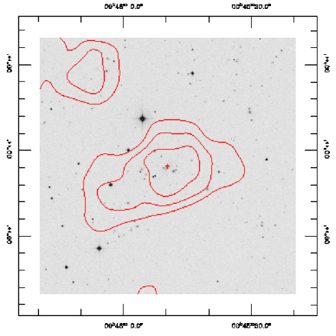
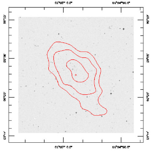
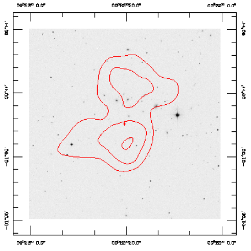
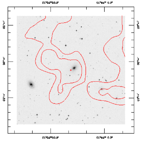
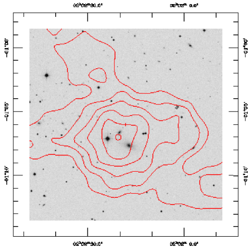
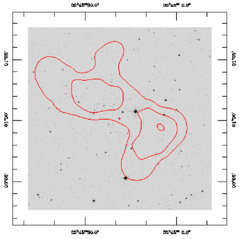
The X-ray/optical overlays in Figs. 10-11 show typical clusters of the present sample. The X-ray data are presented in form of contours of constant signal-to-noise above background in units of $1\sigma,2\sigma,\ldots$. The optical data are from digitized Schmidt plates retrived from the 2nd version of the Digital Sky Survey (DSS2) archive. The clusters RS26, RS53 and RS75 in Fig. 11 are not in the SDSS cluster catalogues of Gogo et al. (2002a) and Bahcall et al. (2003).

All clusters of the present sample show a concentration of optical galaxies towards the X-ray center (in most cases clearly visible even in the less deep DSS2 images). The selection criteria described in Sect. 5 thus appear quite useful: all X-ray cluster candidates passed the visual screening process. We have only excluded 7 targets which were obvious fragments of already detected objects. They could have been excluded already during the source detection in the maximum likelihood maps by introducing a minimum distance between two detected objects. However, from our past experience with NORAS and REFLEX we prefer to reject objects only after a careful visual screening at the end of the complete data processing when all data are in hand.

7 Discussion and conclusions

                                                                                          

Figure 13: X-ray luminosity vs. redshift for the total cluster sample (upper left), for clusters not in the Goto et al. (2002a) sample (lower left), for clusters not in the Bahcall et al. (2003) sample (upper right), and for the clusters neither in Goto et al. and Bahcall et al. (lower right). The redshifts used are estimated from the SDSS data with the matched filter described in Sect. 4.

The present paper describes a method to search for clusters of galaxies by combining data obtained in different energy ranges. The main goal is to reach lower flux limits and to improve the reliability of a first identification of the sources.

As an example, we combined X-ray data from RASS-3 and optical data from SDSS. The SDSS galaxy sample reaches much higher redshifts than RASS and can thus be used to guide a cluster detection in RASS down to lower X-ray flux limits. We could show that a detection of X-ray clusters in RASS-3 is possible down to a nominal X-ray flux limit of $3-5\times 10^{-13}\,{\rm erg}\,{\rm s}^{-1}\,{\rm cm}^{-2}$ in the ROSAT energy band 0.1-2.4 keV. This limit is about 5–10 times deeper than REFLEX and gives a first qualitative impression how much deeper one can get with the new technique.

In the following we discuss the results which are already indicated by the analysis of the test area. Table 2 shows that only 40 out of our 75 X-ray clusters (53%) are listed as X-ray sources in the ROSAT Bright and Faint Source (RBF) catalogues. The overlap can be increased possibly to 73% when a preliminary source list obtained with RASS-3 is used. It is thus not only the X-ray flux limit which can be decreased but also the X-ray completeness which can be increased when RASS and SDSS data are combined.

At the nominal X-ray flux limit only 20% of the 75 clusters show a significant X-ray extent as measured with the GCA method (Fig. 12, Tab. 3). This small fraction is mainly caused by the comparatively small number of source counts (half of the sample has source counts between 5 and 10). Usually, more than 30 source counts are necessary for the GCA method for a significant detection of a source extent – the precise numbers do, however, also depend on the intrinsic extent of the source.

One could worry about a significant contamination by AGN. However, only 12% of the clusters have a known nearby AGN (Tab. 3) and only 5% of the X-ray clusters have an X-ray hardness ratio measured with GCA which is consistent with an AGN (Fig. 12). The fraction of contaminated clusters should thus be not very large, possibly around 10%.

Before we discuss the direct comparisons with published SDSS-based cluster samples we want to note that it would not make much sense to test the number of SDSS clusters which are not present in our sample because SDSS-based cluster surveys are expected to reach much higher redshifts and less rich systems compared to RASS-based cluster surveys. We are thus mainly looking for X-clusters which are not found in SDSS samples.

The comparison of our X-ray cluster sample with public SDSS cluster samples yields the following results: 13 of our 75 X-ray clusters (17%) are not in the catalogue of Goto et al. (2002a) and 23 clusters (31%) are not in the catalogue of Bahcall et al. (2003). At the comparatively bright X-ray fluxes $S\geq 5.0\cdot 10^{-13}\,{\rm erg}\,{\rm s}^{-1}\,{\rm cm}^{-2}$ where spurious detections are unlikely, still 11 clusters (15% of our sample) are not in the Goto et al. sample and 19 clusters (25% of our sample) are not in the Bahcall et al. sample.

However, when we combine the catalogues of Goto et al. and Bahcall et al. then the incompleteness of the optical sample decreases to a level of 8%. The corresponding 6 X-ray clusters which are not in the two SDSS-based cluster catalogues are marked as BG in the last column of Table 2 and have the spectroscopic redshifts $z=0.0637$, 0.0650, 0.0663, 0.0425, 0.0206 and 0.1822. Most of these missing clusters (with one exception) are nearby and less rich systems. This is also seen in the X-ray luminosity/redshift plots shown in Fig. 13. In our X-ray cluster sample we have 12 clusters with redshifts $z<0.07$ and only 7 (58%) are in the combined optical catalogues of SDSS. One should note that the 6 X-ray clusters missing in the optical catalogues on our test area of 140 square degrees could lead to an extrapolated number of 300 clusters over a total SDSS survey area of 7000 square degrees. We are thus discussing here a significant fraction of nearby systems.

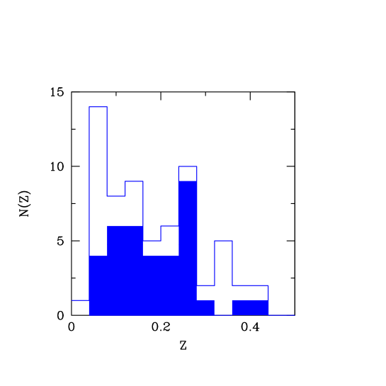
The difference between X-ray and optical cluster selection becomes apparent in Fig. 14, where the redshift distribution of the total sample (unfilled histogram) and the distribution of clusters which are members of both the Goto et al. and the Bahcall et al. samples are compared. Ignoring the redshifts $z>0.3$ where the sample of Bahcall et al. is incomplete (by construction), the redshift distributions are significantly different as seen by the strong deficiency of nearby clusters in the combined Goto plus Bahcall catalogue. Whereas the cluster counts of the combined optical catalogue increase with redshift – which is typical for volume-limited samples – the X-ray sample shows a steady decrease with redshift – which is typical for flux-limited samples. Numerical simulations and comparisons with deep XMM and Chandra observations will give further information about the final incompleteness level which can be reached with our method.

We want to close the discussion of the sample with a few general remarks on the quite deep X-ray flux limit achieved from the combination of RASS and SDSS data. The resulting ‘superfaint’ flux limit – though optimal for the detection of high-redshift clusters and for compiling huge sample sizes – yields X-ray cluster candidates which consists in many cases of only 5–10 RASS X-ray source counts. The corresponding formal flux errors are of the order of 30 and 40%. A careful evaluation of the resulting accuracies achievable in cosmological tests with such samples is thus necessary.

In addition, more work is needed to better calibrate and test our method: (1) The analysis of a larger test area (Data Release 2) is expected to give significantly smaller statistical errors of the cluster number counts which is necessary for a better calibration of the likelihood threshold of the optical data. (2) Tests are under way which quantify the effect an optical sample like SDSS has on the selection of X-ray clusters and vice versa. In Popesso et al. (2004) the correlations between basic optical and X-ray cluster properties are studied and more tests will follow. One of their conclusions is that the $z^{\prime}$ SDSS photometric band and not the $r^{\prime}$ band used here gives the strongest correlations between optical and X-ray data, and should thus be the preferred band when we want to work with the smallest bias caused by including optical data in the detection process. (3) The numerical simulations in Schuecker & Böhringer (1998) have to be performed under the specific conditions of the present survey in order to test selection effects caused especially by the small number of X-ray photons and surface brightness. (4) A direct comparison with ROSAT, XMM-Newton, and Chandra pointed observations will give model-independent estimates of the flux and completeness limits.

7.1 Role of Virtual Observatories

         

Figure 14: Redshift histogram of the clusters with spectroscopic redshifts. Filled steps show the redshift distribution of the clusters which are in common with Goto et al. (2002a) and Bahcall et al. (2003).

The present investigation gives a good illustration of the benefits achievable from the combination of high-quality optical and X-ray data. The combination of the two large databases allows us to fill the gap between nearby wide-angle and deep serendipitous X-ray cluster surveys with already existing data. The combination increases the completeness of the samples and reduces the time-consuming spectroscopic follow-up observations. This method is also expected to be helpful when samples of the order of several $10^{4}$ X-ray cluster candidates expected from future wide-angle X-ray surveys like DUO or ROSITA must be identified.

However, the quality and completeness of the catalogues depends also on the model used to detect and characterize the galaxy clusters. In the present investigation only one set of values of model parameters (cluster core radius, cutoff radius, Schechter characteristic magnitude and faint end slope) was used to develope and illustrate the method. More realistic applications should test different sets of model parameters and use a finer sampling grid for cluster detection. In addition, cluster radii are known to increase with mass so that some kind of iterative procedure is necessary to find the optimal model for each cluster.

Further applications should also include the detection of clusters in so-called Sunyaev-Zel’dovich maps obtained in the centimeter or millimeter range. Such kinds of maps will be provided by, e.g., the PLANCK mission, and will surely increase the reliability of the resulting catalogues.

We are thus left with the conclusion that the quality, the completeness limit, the detection limit, and the telescope time for source identification can be optimized when enough computer power to sample the high-dimensional parameter spaces is available. Moreover, a fast and easy handling of data is needed to work with very large databases probably located at different physical nodes. Virtual observatories like the GAVO provide the infrastructure for such kind of investigation and are surely necessary to make full and efficient use of already existing and future observed data.

GAVO provides an all-sky X-ray event file including many characteristics of the invididual photons. The photons are retrieved from the archive with a general cone-search algorithm. We are currently in the process to implement the cluster search described here within the GAVO grid. This final step is crucial for the analyses of larger survey areas with more cluster models and a finer sampling grid of the detection cells. This will allow us to analyse in a much more efficient manner the SDSS Data Release 2 sample which will become available soon and RASS-3.

The method described in the present investigation needs about 1 hour computing time per square degree on a standard workstation with one processor. Running the method in a controlled manner over a grid of many computers is thus essential for a proper analysis within reasonable times. Our plans include the provision of the cluster (source) detection algorithm as a service of GAVO so that the procedures can be used in a user-friendly manner by a larger community of interested researchers.

Tab. 2. Catalogue of RASS-3/SDSS cluster candidates. Col. 1: Cluster number. Col. 2-3: cluster coordinates in degrees. Col. 4: column density of neutral galactic hydrogen in units of $10^{20}\,{\rm cm}^{-2}$. Col. 5: unabsorbed X-ray flux in units of $10^{-13}\,{\rm erg}\,{\rm s}^{-1}\,{\rm cm}^{-2}$ in the ROSAT energy band 0.1-2.4 keV. Col. 6-7: detection likelihoods on RASS-3 photon maps and SDSS galaxy maps. Col. 8-9: estimated cluster redshifts from RASS-3 and SDSS data. Col. 10: Spectroscopic cluster redshift. Col. 11: Number of cluster galaxies (after rejection of outliners) used for the determination of the spectroscopic cluster redshift. Col. 12: Note whether the cluster is not found in the RASS source catalogues (V), and not found in the SDSS cluster catalogues compiled by Bahcall et al. (B, 2003) and Goto et al. (G, 2002a). For more details see main text.

No.	R.A.	DEC.	$n_{\rm H}$	$S$	$\ln(L/L_{0})$	$\ln(L/L_{0})$	$z_{\rm est}$	$z_{\rm est}$	$z_{\rm spec}$	$N_{z}$	Not in
	2000.0	2000.0			RASS	SDSS	RASS	SDSS			catalogue
RS01	0.3581	-0.0312	3.24	7.39	6.775	19.705	0.40	0.32	0.2578	3
RS02	4.3972	-0.8836	2.95	6.70	7.645	38.440	1.00	0.24	0.2111
RS03	5.0566	0.1015	2.75	7.21	8.094	73.068	0.42	0.20	0.2100	5	G
RS04	5.1680	-0.9858	2.85	5.01	5.202	15.987	1.00	0.06	0.0637	4	V2BG
RS05	5.1943	-1.0844	2.85	3.44	3.184	15.844	1.00	0.08	0.0650	6	V2BG
RS06	5.4073	-0.8459	2.81	4.34	4.007	77.041	1.00	0.08	0.1042	5
RS07	5.6274	-0.9570	2.81	5.35	5.408	29.057	1.00	0.06	0.0581	10	V2B
RS08	5.7515	-0.1543	2.73	6.17	7.786	102.499	1.00	0.18	0.1582	9
RS09	5.7988	0.1977	2.67	7.62	3.360	18.930	0.10	0.22			V2
RS10	7.1309	-0.0857	2.66	3.85	4.616	19.018	1.00	0.06			V2
RS11	7.3730	-0.2509	2.66	16.44	10.839	60.477	0.06	0.08	0.0602	17
RS12	8.0414	-0.6574	2.70	3.10	4.327	19.789	1.00	0.20
RS13	8.5759	0.8777	2.46	6.39	8.643	38.450	0.56	0.20	0.1910	3
RS14	9.3587	0.1414	2.26	3.73	3.384	21.011	1.00	0.12	0.0775	4	G
RS15	10.7036	0.2149	2.20	7.87	6.560	50.102	0.24	0.28	0.2688	2	V23
RS16	10.9596	0.1187	2.18	5.12	4.611	27.796	1.00	0.18	0.2168	4	V23
RS17	11.4570	-0.8486	2.83	13.66	18.840	26.153	0.58	0.12	0.1092	8	G
RS18	11.5751	0.0167	2.23	6.57	7.329	51.584	1.00	0.12	0.1129	15
RS19	11.6170	-0.2219	2.34	6.23	6.697	24.532	0.78	0.18	0.1129	5	V23
RS20	11.8959	-0.8947	2.86	7.15	4.906	21.918	0.18	0.16	0.1178	10	V23
RS21	13.9519	0.6488	2.84	15.83	11.479	37.177	0.08	0.10	0.0695	11	B
RS22	14.0756	-1.1735	3.17	127.50	215.523	45.265	0.08	0.06	0.0447	24
RS23	15.6415	-0.8327	3.68	4.04	3.809	26.316	0.92	0.22	0.2408	4	B
RS24	15.6763	1.1263	3.09	15.81	28.725	60.191	0.24	0.24	0.1437	6
RS25	15.9883	-0.8067	3.46	3.31	3.046	30.689	1.00	0.08	0.0662	9
RS26	16.0781	-0.7695	3.38	5.08	6.110	20.244	1.00	0.04	0.0663	7	BG
RS27	16.0791	-0.4288	3.37	8.30	9.160	41.826	0.24	0.16			G
RS28	16.2231	0.0484	3.42	13.15	20.301	88.368	0.24	0.26	0.2745	4
RS29	16.3765	-0.1699	3.32	7.26	4.274	17.245	0.10	0.20	0.2480	2	V23
RS30	16.5541	0.8009	3.19	25.08	5.004	25.453	0.02	0.26	0.2620	3	V23
RS31	16.7056	1.0513	3.15	33.94	124.722	32.759	1.00	0.22	0.2545
RS32	16.7805	-0.3280	3.34	6.67	7.260	39.992	0.24	0.32	0.2802	2
RS33	17.8626	0.5741	3.08	3.38	4.330	19.399	1.00	0.40	0.4066	2	V23
RS34	18.7749	0.3502	3.38	103.19	128.658	66.772	0.04	0.04	0.0449	27	G
RS35	20.5041	0.3503	3.30	10.18	19.504	47.098	1.00	0.16	0.1751	4
RS36	21.8232	0.3523	3.12	13.25	27.011	51.312	0.52	0.38	0.3437	2	B
RS37	22.0578	-0.6777	3.37	4.07	5.508	18.410	1.00	0.28	0.2566	1	V23
RS38	22.6058	0.4817	2.98	2.92	3.280	19.801	1.00	0.38	0.3365	3	V23B
RS39	22.9211	0.5533	2.93	19.44	24.895	28.408	0.12	0.10	0.0805	11
RS40	23.7341	-0.9379	3.07	3.22	3.001	18.683	0.64	0.08	0.0795	4	B
RS41	24.3671	-0.1861	2.89	4.77	4.817	29.844	1.00	0.46			V2B
RS42	26.6947	-0.6782	2.92	20.10	59.417	20.039	1.00	0.10	0.0825	10	B
RS43	27.2777	-0.4271	2.87	10.01	5.210	17.457	0.06	0.26	0.3336	1	V23B
RS44	27.3363	-1.1850	2.84	3.22	4.958	17.805	1.00	0.50			B
RS45	27.3458	-0.3773	2.86	7.64	4.323	16.164	0.08	0.32	0.3336	1	V23B
RS46	27.8459	-1.0133	2.76	2.95	3.502	16.051	1.00	0.16	0.1209	3	V2
RS47	28.1781	1.0044	2.80	41.83	102.653	138.260	0.20	0.14	0.2300
RS48	28.6185	-0.6531	2.60	4.63	7.332	20.698	1.00	0.40	0.0463	6	B
RS49	29.0463	1.0481	2.87	11.72	13.089	86.197	0.16	0.10	0.0794	22	V2

Tab. 2. Continued

No.	R.A.	DEC.	$n_{\rm H}$	$S$	$\ln(L/L_{0})$	$\ln(L/L_{0})$	$z_{\rm est}$	$z_{\rm est}$	$z_{\rm spec}$	$N_{z}$	Not in
	2000.0	2000.0			RASS	SDSS	RASS	SDSS			catalogue
RS50	29.1534	0.8521	2.79	6.06	10.140	47.039	1.00	0.20	0.2187	4
RS51	29.3443	-0.1020	2.63	3.93	4.010	33.930	1.00	0.42	0.3910	2	V2
RS52	29.4179	-0.1211	2.62	6.44	4.329	36.045	0.14	0.22	0.1352	5	V2G
RS53	30.5762	-1.1003	2.61	37.46	60.376	22.608	0.10	0.06	0.0425	15	BG
RS54	32.7195	-1.1530	2.55	6.87	6.466	24.592	0.28	0.18	0.1731	5	V23
RS55	33.5548	-0.1419	2.76	5.77	5.717	16.778	1.00	0.16	0.1427	6
RS56	34.6231	-0.4454	2.96	5.50	3.012	54.774	1.00	0.24	0.2910	2	V23B
RS57	37.0257	-1.1727	2.68	13.24	10.988	16.801	0.20	0.08	0.0690	14	V23B
RS58	38.9997	-1.0232	2.85	17.24	4.707	16.673	0.12	0.28	0.2470	2	V23
RS59	41.4703	-0.6960	4.02	14.06	5.015	74.357	1.00	0.16	0.1815	6	V2
RS60	42.0287	-0.6403	4.43	11.75	4.911	20.581	1.00	0.02	0.0206		V23BG
RS61	42.3519	1.0279	5.05	13.02	10.612	18.679	1.00	0.38			V2B
RS62	46.0947	1.0847	7.60	5.60	5.436	46.489	1.00	0.12	0.1548		V23
RS63	46.1463	-0.8985	7.02	10.01	10.328	34.808	1.00	0.16	0.1586	3	B
RS64	46.5799	-0.2233	4.99	14.03	4.861	15.094	0.06	0.06	0.1080	11	V23
RS65	47.9288	1.1583	8.16	3.97	4.752	25.775	1.00	0.24	0.2130	1	B
RS66	50.1187	0.5485	7.21	12.23	10.466	23.010	0.20	0.28	0.3851	3	B
RS67	52.0082	0.4007	7.72	4.99	4.947	56.181	1.00	0.26	0.3202	3	V23B
RS68	52.1520	-0.0535	7.60	12.60	21.585	16.214	1.00	0.24			B
RS69	52.6521	-0.5483	7.31	8.90	8.174	19.762	0.22	0.12	0.1487	4	V2B
RS70	53.1336	0.3992	7.73	3.30	3.114	19.936	1.00	0.46	0.4256	3	V2B
RS71	53.5782	-1.1857	7.49	18.42	45.316	33.061	1.00	0.20	0.1387	8
RS72	53.6314	-0.7342	7.88	9.35	12.491	51.521	0.34	0.18			G
RS73	53.9795	-0.6320	8.01	5.58	4.455	20.131	0.22	0.22	0.2741	2	V23
RS74	55.6623	-0.2708	7.79	6.83	5.461	42.824	0.28	0.40			V2B
RS75	56.3280	1.0026	10.60	12.86	6.229	27.567	0.08	0.16	0.1822	4	V2BG

Tab. 3. Catalogue of RASS-3/SDSS cluster candidates. Col. 1: cluster number. Cols. 2-3: cluster coordinates in degrees. Col. 4: source counts. Col. 5: countrates from matched filter and formal $1\sigma$ errors. Col. 6: countrate from Growth Curve Analysis GCA and formal $1\sigma$ errors. Col. 7: normalized hardness ratio (see text). Col. 8: negative logarithmic Kolmogorov-Smirnov probability for a point source. Col. 9: optical richness. Col. 10: further remarks (CONT: AGN within 1 arcmin from cluster position in NED; CUT: cluster only partially in test area of matched filter).

No.	R.A.	DEC.	$N_{\rm ph}$	$\Lambda$	ctr(GCA)	HR	EXT	Richness	Remarks
	2000.0	2000.0		$[{\rm s}^{-1}]$	$[{\rm s}^{-1}]$	GCA	GCA	SDSS
RS01	0.3581	-0.0312	12.5	0.036$\pm 0.010$	0.021$\pm 0.010$	0.59	1.4	79.0
RS02	4.3972	-0.8836	11.3	0.033$\pm 0.010$	0.023$\pm 0.011$	0.75	0.4	90.3	ZwCl 0015.1-0108
RS03	5.0566	0.1015	13.9	0.036$\pm 0.010$	0.026$\pm 0.009$	-1.46	0.2	128.0	RXC00201.1
RS04	5.1680	-0.9858	8.8	0.025$\pm 0.008$	0.018$\pm 0.008$	-1.52	0.0	41.4	2nd CLST $z=0.1071$
RS05	5.1943	-1.0844	6.0	0.017$\pm 0.007$	0.015$\pm 0.007$	0.57	2.1	37.0
RS06	5.4073	-0.8459	8.0	0.021$\pm 0.007$	0.015$\pm 0.007$	-0.27	1.4	113.3	A0023
RS07	5.6274	-0.9570	10.2	0.026$\pm 0.008$	0.026$\pm 0.015$	0.80	0.0	52.3	$z_{\rm G}=0.12921$
RS08	5.7515	-0.1543	12.1	0.030$\pm 0.009$	0.022$\pm 0.010$	0.02	0.1	151.3	A0025
RS09	5.7988	0.1977	14.5	0.038$\pm 0.010$	0.022$\pm 0.010$	-0.30	1.0	62.1	$z_{\rm G}=0.25402$
RS10	7.1309	-0.0857	9.1	0.019$\pm 0.006$	0.013$\pm 0.006$	0.51	0.6	46.8	ZwCl 0025.9-0.021, CONT
RS11	7.3730	-0.2509	39.7	0.081$\pm 0.013$	0.082$\pm 0.018$	-1.11	1.5	92.0	ZwCl 0027.0-0036
RS12	8.0414	-0.6574	9.7	0.015$\pm 0.005$	0.009$\pm 0.005$	-0.54	0.2	56.5	$z_{\rm G}=0.24267$
RS13	8.5759	0.8777	13.6	0.032$\pm 0.009$	0.021$\pm 0.011$	-0.95	1.0	94.2
RS14	9.3587	0.1414	5.8	0.019$\pm 0.008$	0.017$\pm 0.009$	-4.74	0.3	54.0	CONT
RS15	10.7036	0.2149	12.2	0.039$\pm 0.011$	0.027$\pm 0.012$	0.57	0.2	122.2
RS16	10.9596	0.1187	8.1	0.026$\pm 0.009$	0.026$\pm 0.015$	-2.01	2.7	74.3	ZwCl 0041.1-0008
RS17	11.4570	-0.8486	21.3	0.067$\pm 0.015$	0.068$\pm 0.017$	-0.38	1.1	51.8	A0095
RS18	11.5751	0.0167	10.0	0.033$\pm 0.010$	0.028$\pm 0.011$	-0.85	0.1	83.3
RS19	11.6170	-0.2219	9.5	0.031$\pm 0.010$	0.028$\pm 0.011$	0.16	0.3	62.9	$z_{\rm G}=0.26537$
RS20	11.8959	-0.8947	10.5	0.035$\pm 0.011$	0.020$\pm 0.009$	0.28	1.0	49.6	A0101
RS21	13.9519	0.6488	29.1	0.078$\pm 0.014$	0.059$\pm 0.015$	-0.30	2.7	67.1	A0116
RS22	14.0756	-1.1735	207.3	0.621$\pm 0.043$	1.413$\pm 0.071$	0.41	-9.9	56.1	A0119, CUT
RS23	15.6415	-0.8327	7.3	0.019$\pm 0.007$	0.015$\pm 0.007$	0.14	0.0	74.6
RS24	15.6763	1.1263	31.9	0.077$\pm 0.014$	0.060$\pm 0.014$	0.50	1.4	128.8	CONT
RS25	15.9883	-0.8067	6.6	0.016$\pm 0.006$	0.015$\pm 0.015$	-0.50	1.5	64.7
RS26	16.0781	-0.7695	10.3	0.025$\pm 0.008$	0.012$\pm 0.006$	-2.98	0.5	47.5	RASSCALS 087
RS27	16.0791	-0.4288	16.8	0.040$\pm 0.010$	0.023$\pm 0.008$	-0.02	1.1	101.6	CONT
RS28	16.2231	0.0484	26.4	0.064$\pm 0.012$	0.062$\pm 0.013$	-2.45	2.5	174.5	ZwCl 0102.4-0012
RS29	16.3765	-0.1699	14.2	0.035$\pm 0.009$	0.030$\pm 0.019$	-0.60	0.9	64.0	$z_{\rm G}=0.23133$
RS30	16.5541	0.8009	4.1	0.122$\pm 0.019$	0.012$\pm 0.006$	0.11	2.4	90.0
RS31	16.7056	1.0513	69.3	0.165$\pm 0.020$	0.149$\pm 0.020$	-0.55	0.4	84.1	RXCJ 0106.8, CONT
RS32	16.7805	-0.3280	13.4	0.032$\pm 0.009$	0.032$\pm 0.015$	0.12	0.8	139.2	$z_{\rm G}=0.26537$
RS33	17.8626	0.5741	6.9	0.017$\pm 0.006$	0.015$\pm 0.007$	0.37	0.3	104.2	$z_{\rm G}=0.36748$, CONT
RS34	18.7749	0.3502	188.7	0.500$\pm 0.036$	0.435$\pm 0.039$	-3.35	24.9	69.6	A0168, RXCJ0114.9
RS35	20.5041	0.3503	24.5	0.049$\pm 0.010$	0.068$\pm 0.020$	0.82	2.7	86.9	A0181, RXCJ0121.9
RS36	21.8232	0.3523	27.3	0.065$\pm 0.012$	0.059$\pm 0.013$	0.29	2.4	181.7	$z_{\rm G}=0.35613$
RS37	22.0578	-0.6777	8.4	0.020$\pm 0.007$	0.023$\pm 0.011$	-2.47	0.2	66.5	$z_{\rm G}=0.40152$
RS38	22.6058	0.4817	6.1	0.014$\pm 0.006$	0.011$\pm 0.006$	-1.39	0.6	107.2
RS39	22.9211	0.5533	39.1	0.095$\pm 0.015$	0.090$\pm 0.018$	-1.87	5.9	53.1	A0208, RXC0131
RS40	23.7341	-0.9379	6.6	0.016$\pm 0.006$	0.016$\pm 0.007$	-1.70	0.2	46.0
RS41	24.3671	-0.1861	7.0	0.023$\pm 0.009$	0.021$\pm 0.010$	0.62	0.0	162.1	$z_{\rm G}=0.36748$
RS42	26.6947	-0.6782	39.3	0.099$\pm 0.016$	0.081$\pm 0.015$	-4.09	0.1	34.6	CONT
RS43	27.2777	-0.4271	19.6	0.049$\pm 0.011$	0.027$\pm 0.015$	0.29	0.5	64.0	$z_{\rm G}=0.33344$
RS44	27.3363	-1.1850	6.7	0.016$\pm 0.006$	0.023$\pm 0.010$	-0.70	0.1	160.9	$z_{\rm G}=0.29940$
RS45	27.3458	-0.3773	15.3	0.038$\pm 0.010$	0.011$\pm 0.006$	0.16	0.2	81.7	ZwCl 0146.8-0035
RS46	27.8459	-1.0133	6.2	0.015$\pm 0.006$	0.012$\pm 0.006$	-0.94	0.2	44.3
RS47	28.1781	1.0044	85.8	0.206$\pm 0.022$	0.209$\pm 0.027$	-1.93	3.6	180.5	A0267, RXCJ0152.7
RS48	28.6185	-0.6531	9.7	0.023$\pm 0.007$	0.017$\pm 0.007$	0.14	0.0	108.9	$z_{\rm G}=0.43556$
RS49	29.0463	1.0481	23.3	0.058$\pm 0.012$	0.065$\pm 0.016$	0.14	4.2	96.2	A0279

Tab. 3. Continued

No.	R.A.	DEC.	$N_{\rm ph}$	$\Lambda$	ctr(GCA)	HR	EXT	Richness	Remarks
	2000.0	2000.0		$[{\rm s}^{-1}]$	$[{\rm s}^{-1}]$	GCA	GCA	SDSS
RS50	29.1534	0.8521	12.2	0.030$\pm 0.009$	0.023$\pm 0.009$	-0.66	0.0	93.3
RS51	29.3443	-0.1020	8.0	0.019$\pm 0.007$	0.024$\pm 0.014$	-0.08	0.4	174.2
RS52	29.4179	-0.1211	12.7	0.032$\pm 0.009$	0.030$\pm 0.017$	0.15	1.4	97.7
RS53	30.5762	-1.1003	71.2	0.185$\pm 0.022$	0.190$\pm 0.025$	-3.21	4.7	32.9	A0295, RXC0202.3
RS54	32.7195	-1.1530	11.6	0.034$\pm 0.010$	0.027$\pm 0.014$	-0.69	1.6	54.9
RS55	33.5548	-0.1419	7.9	0.028$\pm 0.010$	0.018$\pm 0.009$	-0.91	0.0	48.3
RS56	34.6231	-0.4454	4.8	0.027$\pm 0.012$	0.019$\pm 0.012$	0.31	0.3	122.0
RS57	37.0257	-1.1727	14.3	0.065$\pm 0.017$	0.053$\pm 0.022$	0.83	0.9	25.3
RS58	38.9997	-1.0232	10.6	0.085$\pm 0.026$	0.033$\pm 0.016$	-0.77	2.4	71.1	$t_{\rm eff}=124.8$ s
RS59	41.4703	-0.6960	5.7	0.067$\pm 0.028$	0.033$\pm 0.021$	0.37	0.4	118.7	$t_{\rm eff}=85.8$ s, A0381
RS60	42.0287	-0.6403	6.8	0.055$\pm 0.021$	0.045$\pm 0.020$	-1.33	0.5	39.3	GGrp $z=0.02056$
RS61	42.3519	1.0279	11.5	0.060$\pm 0.018$	0.052$\pm 0.020$	-0.57	0.6	99.5	$z_{\rm G}=0.26537$
RS62	46.0947	1.0847	6.1	0.024$\pm 0.010$	0.016$\pm 0.008$	0.12	1.5	82.4	A0411, RXCJ0304
RS63	46.1463	-0.8985	9.5	0.044$\pm 0.014$	0.034$\pm 0.014$	-0.37	0.4	91.2	CONT
RS64	46.5799	-0.2233	15.3	0.065$\pm 0.017$	0.021$\pm 0.010$	0.16	1.2	37.2	A0412
RS65	47.9288	1.1583	7.5	0.017$\pm 0.006$	0.013$\pm 0.006$	-0.68	0.0	85.5	$z_{\rm G}=0.19729$
RS66	50.1187	0.5485	18.1	0.054$\pm 0.013$	0.042$\pm 0.015$	-0.70	0.3	89.8
RS67	52.0082	0.4007	7.6	0.022$\pm 0.008$	0.014$\pm 0.006$	-1.47	0.0	150.2
RS68	52.1520	-0.0535	19.5	0.055$\pm 0.012$	0.046$\pm 0.013$	0.29	0.6	68.1	$z_{\rm G}=0.26537$, CONT
RS69	52.6521	-0.5483	16.3	0.039$\pm 0.010$	0.019$\pm 0.007$	-0.49	0.9	54.5
RS70	53.1336	0.3992	7.4	0.014$\pm 0.005$	0.011$\pm 0.006$	-1.49	0.0	168.5	$z_{\rm G}=0.39017$
RS71	53.5782	-1.1857	41.9	0.080$\pm 0.012$	0.107$\pm 0.019$	0.24	3.2	86.6	RXCJ0334.0
RS72	53.6314	-0.7342	21.6	0.040$\pm 0.009$	0.037$\pm 0.010$	-0.26	2.0	121.7	$z_{\rm G}=0.41286$
RS73	53.9795	-0.6320	12.3	0.024$\pm 0.007$	0.011$\pm 0.007$	0.02	1.3	71.3	$z_{\rm G}=0.26537$
RS74	55.6623	-0.2708	11.0	0.030$\pm 0.009$	0.016$\pm 0.016$	0.11	0.9	190.7	$z_{\rm G}=0.35613$
RS75	56.3280	1.0026	17.0	0.052$\pm 0.013$	0.013$\pm 0.007$	0.07	3.4	57.3	ZwCl 0342.8+0052