A Limit from the X-ray Background on the Contribution of Quasars to Reionization

Abstract

A population of black holes (BHs) at high redshifts ($z\;\hbox to0.0pt{\lower 2.5pt\hbox{$\sim$}\hss}\raise 1.5pt\hbox{$>$}\;6$) that contributes significantly to the ionization of the intergalactic medium (IGM) would be accompanied by the copious production of hard ($\;\hbox to0.0pt{\lower 2.5pt\hbox{$\sim$}\hss}\raise 1.5pt\hbox{$>$}\;10$ keV) X-ray photons. The resulting hard X–ray background would redshift and be observed as a present–day soft X–ray background (SXB). Under the hypothesis that BHs are the main producers of reionizing photons in the high–redshift universe, we calculate their contribution to the present–day SXB. Our results, when compared to the unresolved component of the SXB in the range 0.5-2 keV, suggest that accreting BHs (be it luminous quasars or their lower–mass “miniquasar” counterparts) did not dominate reionization. Distant miniquasars that produce enough X–rays to only partially ionize the IGM to a level of at most $x_{e}\sim 50\%$ are still allowed, but could be severely constrained by improved determinations of the unresolved component of the SXB.

1 Introduction

The recent discovery of the Gunn–Peterson (GP) troughs in the spectra of $z>6$ quasars in the Sloan Digital Sky Survey (SDSS; White et al. 2003; Wyithe & Loeb 2004) suggests that the end of the reionization process occurs at a redshift near $z\sim 6$. At this epoch, the ionizing sources drive a strong evolution of the neutral fraction of the intergalactic medium (IGM) from values near unity down to $x_{\rm HI}\sim 10^{-3}$ (e.g., Fan et al. 2002). On the other hand, the high electron scattering optical depth, $\tau_{e}=0.17\pm 0.04$, measured recently by the Wilkinson Microwave Anisotropy Probe (WMAP) experiment (Spergel et al. 2003) suggests that ionizing sources were abundant at a much higher redshift, $z\sim 15$. These data imply that the reionization process is extended and complex, and is probably driven by more than one population of ionizing sources (see, e.g., Haiman 2003 for a post-WMAP review).

The exact nature of these ionizing sources remains unknown. Natural candidates to account for the onset of reionization at $z\sim 15$ are massive, metal–free stars that form in the shallow potential wells of the first collapsed dark matter halos (Wyithe & Loeb 2003a; Cen 2003a; Haiman & Holder 2003). The completion of reionization at $z\sim 6$ could then be accounted for by a normal population of less massive stars that form from the metal–enriched gas in larger dark matter halos present at $z\sim 6$.

The most natural alternative cause for reionization is the ionizing radiation produced by gas accretion onto an early population of black holes (“miniquasars”; see Haiman & Loeb 1998, Wyithe & Loeb 2003c, Bromm & Loeb 2003). The ionizing emissivity of the known population of quasars diminishes rapidly beyond $z\;\hbox to0.0pt{\lower 2.5pt\hbox{$\sim$}\hss}\raise 1.5pt\hbox{$>$}\;3$, and bright quasars are unlikely to contribute significantly to the ionizing background at $z\;\hbox to0.0pt{\lower 2.5pt\hbox{$\sim$}\hss}\raise 1.5pt\hbox{$>$}\;5$ (Shapiro, Giroux & Babul 1994; Haiman, Abel & Madau 2001; Wyithe & Loeb 2003a). However, if low–luminosity, yet undetected miniquasars are present in large numbers, they could dominate the total ionizing background at $z\sim 6$ (Haiman & Loeb 1998). Recent work, motivated by the WMAP results, has emphasized the potential significant contribution to the ionizing background at the earliest epochs ($z\sim 15$) from accretion onto the seeds of would–be supermassive black holes (Madau et al. 2003; Ricotti & Ostriker 2003). The soft X–rays emitted by these sources can partially ionize the IGM early on (Oh 2001; Venkatesan & Shull 2001).

A population of miniquasars at $z\;\hbox to0.0pt{\lower 2.5pt\hbox{$\sim$}\hss}\raise 1.5pt\hbox{$>$}\;6$ would be accompanied by the presence of an early X-ray background. Since the IGM is optically thick to photons with energies $E$ below $E_{\rm max}=1.8[(1+z)/15)]^{0.5}x_{\rm HI}^{1/3}\hskip 2.84526pt{\rm keV}$, the soft X-rays with $E\;\hbox to0.0pt{\lower 2.5pt\hbox{$\sim$}\hss}\raise 1.5pt\hbox{$<$}\;E_{\rm max}$ would be consumed by neutral hydrogen atoms and contribute to reionization. However, the background of harder X-rays would redshift without absorption and would be observed as a present–day soft X–ray background (SXB). In this paper, we examine the hypothesis that accreting BHs are the main producers of reionizing photons in the high–redshift universe, and calculate their contribution to the present–day SXB in this case. Our results, when compared to the unresolved component of the SXB, suggest that accreting BHs cannot contribute significantly either to the completion of reionization at $z>6$, or to the partial ionization of the IGM at $z\;\hbox to0.0pt{\lower 2.5pt\hbox{$\sim$}\hss}\raise 1.5pt\hbox{$>$}\;15$ to ionized fractions of $x_{e}\;\hbox to0.0pt{\lower 2.5pt\hbox{$\sim$}\hss}\raise 1.5pt\hbox{$>$}\;0.5$.

The outline of the paper is as follows: In § 2, we describe the method to calculate the SXB from quasars that contribute to reionizing the universe. In § 3, we critically discuss current X-ray observations, focusing on the unresolved fraction of the SXB that could be attributed to distant quasars. In § 4, we calculate the expected contribution to the SXB from hypothetical quasars and their lower–mass miniquasar counterparts that fully ionized the universe. In § 5, we repeat our analysis for a putative miniquasar population that partially ionizes the IGM at high redshifts. In § 6, we discuss how various simplifications made in our analysis influence our final results. Finally, in §7 we summarize our results and the implications of this work. Throughout this paper, we adopt the background cosmological parameters as measured by the WMAP experiment, $\Omega_{m}=0.27$, $\Omega_{\Lambda}=0.73$, $\Omega_{b}=0.044$, and $h=0.71$ (Spergel et al. 2003) and set the mass fraction of helium to $Y_{\rm He}=0.24$ ( e.g. Burles, Nollett, & Turner, 2001). In the rest of the paper ‘accreting BHs’ will refer to both quasars and their lower–mass “miniquasar” counterparts.

2 Modeling the Contribution to the SXB

To calculate the contribution to the present–day SXB from accreting BHs that reionized the universe, we assume for simplicity that the accreting BHs form in a sudden burst at redshift $z=z_{Q}$. The spectrum of the ionizing background is a crucial ingredient of the modeling, and depends on the type of accreting BH that is considered. The details of the assumed emission spectrum for each type are discussed in §4 and 5. In § 6, we examine the dependence of our results on the emission spectrum.

Assuming that the cumulative hard X–ray flux of the accreting BHs results in a present–day X-ray background $F_{E}$, we can compute the number of H–ionizing photons present at redshift $z_{Q}$ per unit comoving volume:

$$n_{\gamma}=\frac{4\pi}{c}\int_{\frac{13.6}{1+z_{Q}}\rm{eV}}^{\frac{E_{\rm{max}}}{1+z_{Q}}\rm{eV}}dE\frac{F_{E}}{E}$$ (1)

In the above equation, $E$ and $F_{E}$ correspond to photon energies and intensities at $z=0$, and $F_{E}$ has the units of ${\rm ergs~{}cm^{-2}~{}s^{-1}}$ $\rm{~{}deg^{-2}~{}erg^{-1}}$. The photon energy $E_{\rm max}=1.8[(1+z)/15)]^{0.5}\hskip 2.84526pt{\rm keV}$ reflects the value above which the IGM becomes optically thin across a Hubble length for a fully neutral IGM. For most spectral slopes in the range we study here, we have verified that our results are insensitive to the choice of $E_{\rm max}$. The exception is in §5, where we consider unusually hard spectra; in this case the exact value of $E_{\rm max}$ does influence the results. A brief discussion of this will be given in §5.

The total number of H–ionizations per unit comoving volume is approximately equal to the comoving density of H–ionizing photons $n_{\gamma}$ with energy below $\approx E_{\rm max}$. This simple formulation ignores secondary ionizations by the photo–electrons produced by the more energetic photons ($E\gtrsim 100$ eV). For spectra of the form $F_{E}\propto E^{-\alpha}$ with $\alpha>0.7$ at $E>13.6$ eV, these secondary ionizations are subdominant compared to the ionizations by the UV–photons (Abel et al. 1997). More importantly, the number of secondary ionizations is negligible for any spectrum if the ionized medium has a neutral fraction, $x_{\rm HI}\ll 1$ (since the electron energy is instead used to heat the gas; e.g. Shull & van Steenberg, 1985). For harder spectra and a partially ionized medium, secondary ionizations become important. We will return to this issue in § 5 below, where we discuss a miniquasar population that is assumed to only partially ionize the IGM.

Since helium may be reionized later by the already known population of optical quasars at $z\sim 3$ (Sokasian, Abel & Hernquist 2002; Wyithe & Loeb 2003a), we consider only hydrogen here. The presence of helium will not significantly change our results, as will be discussed in §6.2 below.

The normalization of the present–day background $F_{E}$ is obtained by requiring that the quasar population would lead to reionization,

$$n_{\gamma}=\eta n_{H,0}$$ (2)

where $n_{H,0}=\Omega_{b}h^{2}\rho_{\rm crit}(1-Y_{\rm He})/m_{p}=2.05\times 10^{-7}\hskip 2.84526pt\rm{cm}^{-3}$ is the number density of H–atoms at $z=0$ and $\eta$ is the number of ionizations per hydrogen atom that are required to achieve reionization.

The value of $\eta$ is larger than unity because of the need to balance recombinations. The ratio between the Hubble time, which is taken to be $t_{\rm hub}(z)\equiv 2H^{-1}(z)/3$, and the recombination time in a region at overdensity $\delta$ that is partially ionized to $x_{H^{+}}\equiv n_{H^{+}}/n_{H}$, where $n_{H}$ is the number density of hydrogen atoms (neutral and ionized) at any redshift $z$, is given by:

$$\frac{2H^{-1}}{3t_{\rm rec}}=1.7\hskip 2.84526ptC\hskip 2.84526pt\Big{(}\frac{10^{4}}{T}\Big{)}^{0.7}\Big{(}\frac{1+z}{11}\Big{)}^{1.5}x_{e}\hskip 2.84526pt(1+\delta)$$ (3)

Where $x_{e}\equiv n_{e}/n_{H}$ ($=x_{H^{+}}$, because helium is not included), $C\equiv\langle n^{2}\rangle/\langle n\rangle^{2}$ which depends on the level of clumping in the high–redshift the IGM, and is expected to be $\gtrsim 10$ (Haiman, Abel, & Madau 2001; Wyithe & Loeb 2003a; Ricotti & Ostriker 2003), and $T$ is the gas temperature. This implies that recombinations cannot be ignored at high redshift. In fact, the number of recombinations per hydrogen atom between $z=z_{Q}$ and $z=7$, $N_{\rm rec}$, can be estimated from

$$N_{\rm rec}\hskip 2.84526pt\equiv\hskip 2.84526pt\int_{t(z=z_{Q})}^{t(z=7)}\frac{\alpha_{H}(T)\hskip 2.84526ptn_{e}\hskip 2.84526ptn_{H^{+}}}{n_{H^{+}}}dt$$ (4)

Interestingly, for any combination of $z_{Q}$ and $x_{e}$ yielding the same $\tau_{e}$, this can be written as a function of $\tau_{e}$ as long as $x_{e}$ is constant with redshift for $z>7$ and $x_{e}\sim 1$ for $0<z<7$:

$$N_{\rm rec}=2.4\hskip 2.84526ptC\hskip 2.84526pt(1+\delta)\Big{(}\frac{T}{10^{4}}\Big{)}^{-0.7}\Big{(}\frac{\tau_{e}-0.05}{0.12}\Big{)},$$ (5)

where $\tau_{e}$ is the electron scattering optical depth between redshifts $z=0$ and $z=z_{Q}$. Note that $x_{e}\sim 1$ for $0<z<7$ and $x_{e}=0$ for $z>7$ yields $\tau_{e}=0.05$. The recombination coefficient $\alpha_{H}(T)$ is taken from Abel et al. (1997). To maintain a fixed ionization fraction we need $\eta\equiv N_{\rm rec}+1\sim 25$ ionizations per hydrogen atom. In §6.5 we will show that the actual value of $\eta$ depends on the exact topology of reionization, and therefore quite uncertain. The SXB intensity $F_{E}$ predicted below simply scales linearly with the exact value of $\eta$. Given the uncertainty in $\eta$ we will adopt the fiducial value of $\eta=10$, and scale our quoted fluxes in units of $(\eta/10)$ (see Table 2).

It is important to emphasize that we are normalizing $F_{E}$ based on the total ionizing background, required to produce reionization. Our prediction for $F_{E}$ therefore does not require the knowledge of the luminosity function of the quasars.

3 The Unresolved SXB and Its Uncertainties

Since the unresolved fraction of the SXB is the key observable used to obtain the constraints in this paper, we first discuss its measurement and uncertainty. The soft X-ray band in the energy range $0.5-2.0$ keV has been studied by Moretti et al. (2003, hereafter M03). We focus on this energy range since it provides the strongest constraints. The $0.5-2$ keV band corresponds to hard X–rays at $z\geq 6$, which are well within the regime of photon energies to which the IGM is optically thin. M03 determines the intensity of the total SXB within this band to be $\int F_{E}dE\sim EF_{E}(1\hskip 2.84526pt\rm{keV})$ = $7.53\pm 0.35\times 10^{-12}$ $\rm{ergs}\hskip 2.84526pt\rm{cm}^{-2\hskip 2.84526pt}\rm{s}^{-1}\hskip 2.84526pt\rm{deg}^{-2}$ , when combining 10 different measurements reported in the literature. M03 further include deep pencil beam surveys together with wide field shallow surveys and ultimately are able to identify discrete sources in the flux range $2.44\times 10^{-17}-1.00\times 10^{-11}$ $\rm{ergs}\hskip 2.84526pt\rm{cm}^{-2\hskip 2.84526pt}\rm{s}^{-1}$  within the soft band. They find that $94^{+6}_{-7}\%$ of the SXB is made up of discrete X-ray sources. The majority of this resolved component involves point sources ($88\pm 7\%$ of the total SXB), with extended sources amounting to $6\%$ of the background. Barger et al. (2002, 2003) show that the bulk of these sources are at low redshifts, $z<4$. In § 6.4 below we find that any $z\geq 6$ quasars that “hide” among the already resolved point sources can only make up to $1\%$ of the total SXB.

The fraction of the SXB contributed by known discrete (point or extended) sources depends on the sensitivity limits of current observations. M03 find that when they extrapolate the analytic form of the log N-log S distribution (cumulative fraction of the total SXB in sources brighter than flux S) to $S_{\rm min}\sim 3\times 10^{-18}~{}{\rm ergs~{}s^{-1}~{}cm^{-2}}$, which is a factor of $\sim$ 10 lower than current sensitivity limits, the entire SXB can be accounted for by discrete sources. The additional, still undetected faint X–rays sources could be either point–like or extended.

Wu & Xue (2001) calculate the theoretically expected amount of X–ray emission in the soft band from thermal emission by gas in all clusters and groups in the universe using the observed $L_{X}-T$ relation and X–ray luminosity function (XLF) and find this should be $1.18\times 10^{-12}$ $\rm{ergs}\hskip 2.84526pt\rm{cm}^{-2\hskip 2.84526pt}\rm{s}^{-1}\hskip 2.84526pt\rm{deg}^{-2}$ . This is $16\%$ of the total SXB quoted by M03. Approximately $\sim 40\%$ of this contribution originates in galaxy groups; ignoring groups (where the XLF extrapolation becomes uncertain) provides a conservative estimate of the total expected contribution from thermal emission from extended sources, $\sim 0.6\times 1.18\times 10^{-12}=0.68\times 10^{-12}$ $\rm{ergs}\hskip 2.84526pt\rm{cm}^{-2\hskip 2.84526pt}\rm{s}^{-1}\hskip 2.84526pt\rm{deg}^{-2}$ , which is $9\%$ of the total SXB. This suggests that the actual contribution to the SXB from extended sources is higher than claimed by M03, and that deeper X–ray observations will reveal new extended X–ray sources at flux levels below current sensitivity limits. To remain conservative we take the M03’s estimate of $6\%$ for the contribution of extended sources to the SXB, but keep in mind that the actual number is probably higher, leaving a smaller residual that can be attributed to distant accreting BHs.

Recent numerical simulations by Davé et al. (2001) suggest that a fraction as large as 0.3-0.4 of all baryons might be in the warm/hot intergalactic medium (WHIM) with temperatures between $10^{5}-10^{7}$K, residing in diffuse large scale structures such as the filaments connecting virialized objects at $z=0$. The WHIM should emit some thermal radiation in the soft X–ray band, but has so far not been detected. In this paper, we ignore the possible contribution to the SXB from the WHIM. Note that any WHIM contribution would strengthen our results, since it would again leave a smaller residual of the SXB that can be attributed to distant accreting BHs.

Soltan (2003) pointed out that point sources can never make up the full SXB, because the X-ray photons will be Thompson scattered by free electrons, yielding a diffuse component. This component is estimated to be $\sim 1.0-1.7\%$ of the total SXB. Although this is a small fraction, it makes a non-negligible contribution to the unresolved SXB, and we include it in our analysis below.

A summary of the possible SXB contributions is given in Table 1. The Table quotes an intensity for a “mean” and a “maximum” unaccounted SXB flux. The mean unaccounted flux is the total flux minus the contributions from point sources, galaxy clusters, and Thompson scattered X-rays. The maximum unaccounted flux is calculated by summing the $1\sigma$ errors ($3^{{\rm rd}}$ column in Table 1) in the most conservative way: the total SXB is set to its maximum ($+1\sigma$) value, while all other components (point sources, extended sources and scattered X–rays) subtracted from this total are assumed to be at their minimum ($-1\sigma$) levels. We find the mean and maximum unaccounted fluxes to be $0.35\times 10^{-12}$ $\rm{ergs}\hskip 2.84526pt\rm{cm}^{-2\hskip 2.84526pt}\rm{s}^{-1}\hskip 2.84526pt\rm{deg}^{-2}$ and $1.23\times 10^{-12}$ $\rm{ergs}\hskip 2.84526pt\rm{cm}^{-2\hskip 2.84526pt}\rm{s}^{-1}\hskip 2.84526pt\rm{deg}^{-2}$ , respectively.

It should be noted that a similar analysis can be done for the hard X–Ray background (2.0-8.0 keV), but since the constraints in this band are considerably weaker, we do not discuss them here.

Table 1: Contributions to the Soft X-ray Background

Source	Flux	$\sigma_{\rm flux}$
	($10^{-12}$ $\rm{ergs}\hskip 2.84526pt\rm{cm}^{-2\hskip 2.84526pt}\rm{s}^{-1}\hskip 2.84526pt\rm{deg}^{-2}$ )
Total SXB	7.53	0.35
Point Sources	6.63	0.35
Diffuse Component	0.45	0.25
Expected scattered background	0.10	0.03
Unaccounted flux (mean)	0.35	0.60
Unaccounted flux (max)	1.23

4 Full Reionization by the UV Emission of Accreting Black Holes

4.1 Reionization by Quasars

We follow the procedure outlined in §2 and calculate the present day SXB, $F_{E}$, for a burst of quasars at redshifts $z_{Q}=6,10$ and 20, assumed to fully reionize the universe. We adopt the shape of the fiducial quasar spectrum from Sazonov, Ostriker, & Sunyaev (2004, see their eqs. 8 and 14), which is then assumed to redshift to $z=0$ without absorption for hard X-rays. This broad–band spectral energy distribution of the average quasar in the universe is computed based on a detailed theoretical model that fits a range of data, including published composite spectra of quasars in the optical, UV and X–ray bands. The template spectrum scales approximately as $F_{E}\propto E^{-1.7}$ for $E>13.6$ eV, but becomes much shallower beyond $E=2$ keV, where it scales as $F_{E}\propto E^{-0.25}$. The main reason for this ’kink’ in the spectrum around $E=2$ keV is to accommodate the rise in the observed cosmic X–ray background in the energy range 1-30 keV.

The resulting flux density is plotted in the range 0.1–10 keV in Figure 1, assuming $\eta=10$, with the upper curve corresponding to $z_{Q}=6$, and the lower curve to $z_{Q}=20$. The $EF_{E}$ curves are redshifted and suppressed by a factor of $(1+z_{Q})$ relative to the rest–frame template spectrum (which peaks at $E=60$ keV). As a result, we obtain the largest SXB for the quasar burst at the low end of the redshift range, $z_{Q}=6$.

The two straight lines plotted in the range 0.5-2.0 keV denote the mean and maximum unaccounted flux of Table 1. The unaccounted flux is assigned a power-law spectrum with a slope matching the spectral slope of quasars in the range $0.5-2.0$ keV. The figure shows that at all three redshifts, the SXB intensity significantly exceeds the level of the mean unaccounted flux (by a factor of $\sim 4-6$), and is above our inferred maximum level. To compare directly with the values quoted in Table 1 we calculate $F_{\rm QSO}\equiv\int_{0.5\rm{keV}}^{\rm{2.0keV}}F_{E}dE$. For $z=6,10,$ and $20$, we find $F_{\rm QSO}=2.17,1.84,$ and $1.37\hskip 2.84526pt$ $\times 10^{-12}(\eta/10)$ ${\rm ergs~{}cm^{-2}~{}s^{-1}~{}deg^{-2}}$, respectively. For any redshift, the maximum unaccounted flux is saturated.

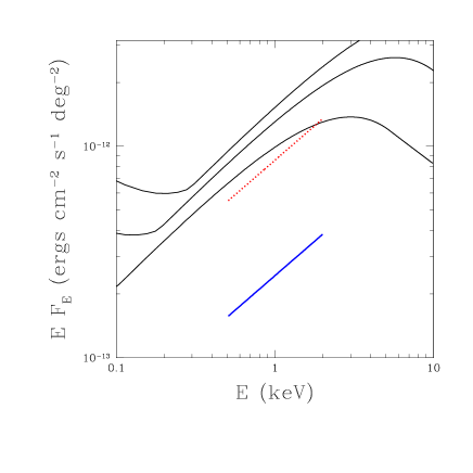
Figure 1: Predicted soft X-ray background due to a burst of quasars producing $\eta=10$ ionizing photons per hydrogen atom and reionizing the universe at $z=6,10$ and $20$ (first three curves from the top). The template spectrum for these quasars is taken from Sazonov, Ostriker, & Sunyaev (2004). The two straight lines plotted in the range 0.5-2.0 keV are the maximum and mean unaccounted flux in the observed soft X-ray background (Table 1). A power-law spectrum is assigned to this flux, with a slope matching the spectral slope of quasars.

4.2 Reionization by Miniquasars

In the previous section, we addressed the scenario in which the IGM is fully ionized by luminous quasars. An alternative scenario is that in which the ionizing background is dominated by accretion onto the much less massive seed BHs that later grow to be the massive BHs powering luminous quasars. The main difference, for our purposes, is the typical spectrum of the ionizing sources in the two scenarios. Our fiducial template from Sazonov, Ostriker, & Sunyaev (2004) that we used above is appropriate for luminous quasars at lower redshifts ($0<z<5$), powered by supermassive black holes with masses of $M_{\rm bh}\approx 10^{6-9}$ $M_{\odot}\hskip 2.84526pt$. The spectra of miniquasars, with BHs whose masses are in the range $M_{\rm bh}\approx 10^{2-4}$ $M_{\odot}\hskip 2.84526pt$(Madau et al, 2003) are likely to be harder.

To obtain the spectrum of a typical miniquasar, we follow the approach of Madau et al. (2003) and adopt a template that consists of two components. One component originates from a multi color accretion disk (MCD), which describes the accretion disk as series of blackbody annuli with different temperatures, and results in a spectrum that scales as $F_{E,{\rm MCD}}\propto E^{1/3}$ up to $kT_{\rm max}=1\rm{keV}\hskip 2.84526pt(M_{\rm bh}/M_{\odot})^{-1/4}$. The second component is a simple power-law $F_{E,{\rm PL}}\propto E^{-1}$ for $E>13.6$ eV. The precise origin of this power–law emission is not fully understood, but is likely to be a combination of Bremsstrahlung, synchrotron, and inverse Compton emission by a non-thermal population of electrons.

This power-law + MCD composite model adequately describes some ultraluminous X-ray sources (ULXs), that are claimed to be associated with an intermediate mass black hole of $\sim 10^{3}$ $M_{\odot}\hskip 2.84526pt$(Miller et al. 2003). In these spectra the flux from the MCD, $F_{\rm MCD}$ , is comparable to the flux in the power–law component, $F_{\rm PL}$. Miller et al. (2003) find the ratio of $F_{\rm PL}$ to the total flux to be 0.33 and 0.63 for the two ULX sources NGC 1313 X–1 and X–2 respectively. Motivated by these observations, here we take $F_{\rm MCD}\equiv\int_{0.0136~{}{\rm keV}}^{kT_{\rm max}}F_{E,{\rm MCD}}dE$, $F_{\rm PL}\equiv\int_{0.2~{}{\rm keV}}^{10~{}{\rm keV}}F_{E,{\rm PL}}dE$, and define the ratio $\Psi\equiv F_{\rm MCD}/F_{\rm PL}$. In this paper, we adopt $\Psi\equiv 1$, and vary it between 0.5 and 2.0 as an additional source of uncertainty.

An additional source of uncertainty is the mass of the typical black hole, $M_{\rm bh}$. Madau et al. (2003) show the mass function of accreting intermediate mass black holes at four different redshifts. The median mass at $z=22$ is $M_{\rm bh}\sim 100\hskip 2.84526ptM_{\odot}$, increasing to $\sim 1000\hskip 2.84526ptM_{\odot}$ at $z=13$. To approximately mimic this increase, we adopt $\log(M_{\rm bh})=(4.1-0.1z)\pm 0.5$. The error in the black hole mass is incorporated into the error in the final contribution to the SXB.

Applying the analysis outlined in § 2 with this modified spectral shape yields $F_{\rm mQSO}\equiv\int_{0.5\rm{keV}}^{\rm{2.0keV}}F_{E}dE$ = $3.3\pm 1.1$, $2.3\pm 0.8$ and $1.4\pm 0.4\hskip 2.84526pt$ $\times 10^{-12}(\eta/10)$ $\rm{ergs}\hskip 2.84526pt\rm{cm}^{-2\hskip 2.84526pt}\rm{s}^{-1}\hskip 2.84526pt\rm{deg}^{-2}$ for $z=6,10$ and $20$, respectively. The dominant contribution to our quoted error is the uncertainty in $\Psi$, the relative importance of the flux in the power law component to the flux from the MCD component. Despite the differences in the assumed spectra for quasars and miniquasars, their contribution to the current SXB, under the assumption that they fully ionized the IGM, is comparable. For any redshift, we find that miniquasars saturate the mean unaccounted flux of the SXB. Only for $z=20$ the maximum unaccounted flux of the SXB is not saturated within the uncertainty of our model.

5 Partial “Preionization” by X–rays from Miniquasars

We have so far omitted secondary ionizations from our analysis. Secondary ionizations are collisional ionizations by the photo–electron that is knocked off the hydrogen atoms when ionized by energetic X–ray photons. Shull & van Steenberg (1985) quantify the fraction $\phi(x_{H^{+}},E)$ of the energy of these electrons that is used for H–ionizations. They find that for energies $\gg 100$ eV, $\phi(x_{H^{+}},E)$ is independent of energy, and $\phi(x_{H^{+}},E)\sim 1/3$ for a neutral medium ($x_{H^{+}}=0$) although it drops rapidly for $x_{H^{+}}\gtrsim 0.1$. This justifies for our statement in § 2 that secondary ionizations do not contribute significantly to full reionization (as we further show in more detail at the end of this section). However, secondary ionizations can become significant in a partially ionized medium, especially for harder spectra.

The large electron scattering optical depth WMAP result can be explained with a partially ionized IGM, followed by full reionization at $z\lesssim 6.3$ (e.g. Wyithe & Loeb 2003b, 2004; Cen 2003b; Haiman & Holder 2003). For example, reionization up to an ionized fraction $x_{e}=0.3,0.5.$ and $0.7$ at $z_{Q}=34,24,$ and $20$, respectively, with $x_{e}=const$ down to $z\sim 7$ and $x_{e}\sim 1$ at $0<z\lesssim 7$ yields $\tau_{e}=0.17$ (Ricotti & Ostriker 2003). In these preionization scenarios, secondary ionizations are important because the quasar spectrum is significantly harder and consists primarily of X–rays. Since helium is ignored, $x_{e}=x_{H^{+}}$. In §6.2 we demonstrate that including helium does not change the final results by more than $\sim 15\%$.

X–rays may have some advantages in partially reionizing the universe (Oh 2001; Venkatesan, Giroux, & Shull 2001; Ricotti & Ostriker 2003). First, for low ionization states of a gas ($x_{H^{+}}\lesssim 0.1$), a single X–ray photon can produce multiple secondary ionizations. Also, the escape fractions of X–rays from the local high density environments of sources into the lower density regions, is high: $f_{\rm esc}\sim 1$. In these low density regions, the clumping factor $C$ is expected to be $\sim 1$.

This implies that, contrary to the case of full ionization by UV–photons, which requires $\eta\gtrsim 10$ photons per baryon (§2), partial ionization to a fraction $x_{H^{+}}$ by X–ray photons requires only $\eta=x_{H^{+}}(1+N_{\rm rec})/(1+\mathcal{N}_{\rm sec})$, where $\mathcal{N}_{\rm sec}$ is defined to be the mean number of secondary ionizations caused by a single photon (given below in eq. [9]). In the preionization models of Ricotti & Ostriker (2003) a considerably harder template spectrum is used, with $F_{E}\propto E^{4}$ at $E<100$ eV, and $\propto E^{-1}$ at $E>100$ eV, as appropriate for highly obscured sources. A physical motivation for the break at this energy is that the column density of isothermal gas in hydrostatic equilibrium in a typical virialized halo at $z=10-20$ is $N_{\rm HI}\sim 10^{20-21}\hskip 2.84526pt{\rm cm}^{-2}$ (Dijkstra et al. 2004). Photons with $E\gtrsim 150\hskip 2.84526pt\rm{eV}\hskip 2.84526pt(N_{\rm HI}/10^{20}\hskip 2.84526pt{\rm cm}^{-2})^{1/3}$ can escape unimpeded from a halo, whereas the halo is optically thick to less energetic photons.

In order to repeat the analysis of §2 with the modified spectrum and the secondary ionizations included, we first compute the mean number of secondary ionizations per photon, $\mathcal{N}_{\rm sec}$. The total number of ionizations per unit comoving volume to go from electron fraction $x_{e}$ to $x_{e}+dx_{e}$ is:

$$dn_{\rm Hion}=(1+N_{\rm rec})\hskip 2.84526ptdx_{e}\hskip 2.84526ptn_{H,0}$$ (6)

The number of hydrogen ionizations per comoving volume is given by:

$$n_{\rm Hion}=n_{\gamma}\Big{(}1+\frac{1}{n_{\gamma}}\frac{1+z}{13.6\hskip 2.84526pt\rm{eV}}\frac{4\pi}{c}\int_{\frac{13.6}{1+z}\rm{eV}}^{\frac{E_{\rm{max}}}{1+z}\rm{eV}}dE\hskip 2.84526ptF_{E}\times\hskip 2.84526pt$$

$$\times\phi[E(1+z)-13.6\hskip 2.84526pt\rm{eV},x_{e}]\Big{)}\equiv n_{\gamma}[1+\langle\mathcal{N}_{\rm sec}\rangle(x_{e})]$$ (7)

In this equation, $n_{\gamma}$ is the comoving number density of H–ionizing photons (eq. 1). As mentioned above, the more energetic photons of energy $E$ will produce a secondary photo–electron of energy $E-13.6\hskip 2.84526pt\rm{eV}$, which will spend a fraction $\phi(E-13.6\hskip 2.84526pt\rm{eV},x_{e})$ of its energy on H–ionizations. The fitting formula we used for $\phi(E,x_{H^{+}})$ in our numerical integration is described in the Appendix. Note that we can only write $x_{e}$ here because it is equal to $x_{H^{+}}$ (see §6.2 for the effect of helium). The quantity $\langle\mathcal{N}_{\rm sec}\rangle$ $(x_{e})$ denotes the mean number of secondary ionizations per photon over the entire energy range at electron fraction $x_{e}$. The above equation simply states that each H–ionizing photon produces one primary and $\langle\mathcal{N}_{\rm sec}\rangle$ $(x_{e})$ secondary ionizations, when the electron fraction in the gas is $x_{e}$. Note that the primary ionizations are actually driven by helium, but as argued in §6.2 this only slightly changes our final results.

Combining equations (6) and (7), we require for the number of ionizing photons per comoving volume

$$dn_{\gamma}(x_{e}\rightarrow x_{e}+dx_{e})=\frac{(1+N_{\rm rec})\hskip 2.84526ptn_{H,0}\hskip 2.84526ptdx_{e}}{1+\langle\mathcal{N}_{\rm sec}\rangle(x_{e})}.$$ (8)

The total number of ionizing photons per comoving volume, $n_{\gamma,\hskip 2.84526pt\rm{tot}}$, to change the ionized fraction from $0$ to $x_{e}$ can be obtained by integrating equation (8) from $0$ to $x_{e}$.

$$n_{\gamma,\hskip 2.84526pt\rm{tot}}\equiv\frac{(1+N_{\rm rec})\hskip 2.84526ptx_{e}\hskip 2.84526ptn_{H,0}}{1+\mathcal{N}_{\rm sec}},$$ (9)

in which the number $\mathcal{N}_{\rm sec}$ is the mean number of secondary ionizations per photon over the whole energy and electron fraction range. This is the number we referred to earlier in this section.

To show the relative importance of secondary ionizations, we list the values of $\mathcal{N}_{\rm sec}$ in Table 2. Note that these numbers are slightly higher than those in Madau et al. (2003). The main reason is that our number is mean number of secondary ionizations per photon over the whole electron fraction range up to $x_{e}$, whereas their number is given at the specific value $x_{e}$.

Given $\mathcal{N}_{\rm sec}$, we set $\eta=x_{e}(1+N_{\rm rec})/(1+\mathcal{N}_{\rm sec})$ and calculate the present-day SXB intensity for the three preionization scenarios with different $x_{e}$ and reionization redshift, as considered by Ricotti & Ostriker (2003). The fluxes we find are listed in Table 2. As the table shows, models within which X–rays are assumed to partially ionize the IGM to $x_{e}\lesssim 0.5$ do not saturate the mean unaccounted SXB. The preionization scenario with $x_{e}=0.7$ has a similar contribution to the SXB as the models that aim for full reionization and saturates the maximum unaccounted flux.

As mentioned in §2 the results are dependent on the exact value of $E_{\rm max}$, being the energy below which photons would typically be absorbed and contribute to H-reionization at any redshift prior to $z\approx 6$, for a partially ionized IGM. The optical depth of a partially ionized IGM between $z=z_{Q}$ and $z=6$ for a photon of energy $E$ emitted at $z=z_{Q}$ is,

$$\tau(E)=\frac{c}{H_{0}\sqrt{\Omega_{m}}}\int_{6}^{z_{Q}}\frac{dz}{(1+z)^{5/2}}\big{[}n_{HI}\sigma_{H}(E^{\prime})+n_{HeI}\sigma_{He}(E^{\prime})\big{]},$$ (10)

where $E^{\prime}=E(1+z)/(1+z_{Q})$ and $n_{HI}\hskip 2.84526pt(n_{HeI})$ is the proper number density of neutral hydrogen (helium) atoms. Although helium has been ignored in this section, it is included in this formula since it dominates the contribution to $\tau(E)$ for X–ray photons. We discuss the implications of helium in more detail in §6.2. The cross–sections are taken from Verner et al. (1996).

The value of $E_{\rm max}$ was obtained by setting, $\tau(E_{\rm max})\equiv 1$. There is some arbitrariness in this definition, and to check how it affects our results we repeated our analysis using $E_{\rm max,alt}$ defined by $\tau(E_{\rm max,alt})\equiv 0.1$. This roughly corresponds to doubling $E_{\rm max}$ and brings down our calculated contributions to the SXB by $\lesssim 15\%$. Since this choice of $E_{\rm max,alt}$ is very unrealistic (photons of energy $E_{\rm max,alt}$ are only absorbed $\sim 10\%$ of the time) we believe that the actual choice of $E_{\rm max}$ is influencing our results by less than $\sim 15\%$.

Using the model for secondary ionizations, we can calculate their contribution for the full reionization cases described in §4. We find that for the quasar case (§4.1), $\mathcal{N}_{\rm sec}\lesssim 0.04$, which is a negligible contribution. For the miniquasars, with harder spectra, $\mathcal{N}_{\rm sec}\lesssim 0.10$, which would come down to a $\sim 10\%$ reduction in the calculated contribution to the SXB. Since the errors in these contributions were of the order of $\sim 30\%$, ignoring the contributions from secondary ionizations is justified.

6 Discussion

6.1 Constraints on Spectrum

As emphasized above, the spectral shape of the putative typical high–$z$ accreting BH is uncertain; the existing templates, motivated by lower–redshift sources, can be considered merely as guides. In this section, we adopt a different strategy and ignore any physically motivated features in the spectrum. Instead, we adopt a simple power–law shape, $F_{E}\propto E^{-\alpha}$ for $E>13.6$ eV. We then consider a range of values for $\alpha$, and also vary $\eta$ (eq. 2) to calculate the contribution to the SXB. Figure 2 shows which combinations of $\alpha$ and $\eta$ value (Eq. 2) are allowed by the mean and maximum unaccounted flux in the SXB (see Table 1). The solid (dotted) lines denote those models with combinations of $\alpha$ and $\eta$ such that the predicted contribution to the SXB is equal to the mean (maximum) unaccounted flux. The redshift of the burst of accreting BH formation in this case is assumed to be $z_{Q}=10$.

This figure shows that for $\eta=10$, which was used in §4.1 and §4.2, any power–law shallower than $\alpha\approx 1.4$ (1.2) will saturate the mean (maximum) unaccounted flux. This figure also demonstrates that when $\alpha=1$, the mean (or maximum) unaccounted flux is saturated when $\eta$ is greater than 1 (or 4).

Figure 2: Constraints on the number of ionizing photons per H atom, $\eta$, (eq. 2) and the power–law index for the slope of the ionizing background, $\alpha$, based on the intensity of the present–day SXB. The quasars are assumed to form at $z_{Q}=10$ and have a power–law spectrum, $F_{E}\propto E^{-\alpha}$ for $E>13.6$ eV. The curves bracket the allowed parameter space for the mean (solid line) or maximum (dotted) unaccounted flux in the SXB.

6.2 The Influence of Helium

So far our analysis has ignored the presence of helium for simplicity. In this section we will demonstrate how the presence of helium reduces the contribution of accreting black holes to the SXB, albeit at a level $\lesssim 15\%$.

The photoionization cross–section for neutral (and singly ionized) helium, $\sigma_{\rm He}$ (and $\sigma_{\rm He^{+}}$) is significantly larger in the X–rays than that for hydrogen, $\sigma_{H}$. For example, for $E=100$ eV $\sigma_{\rm He}/\sigma_{H}\sim 20$ and for greater energies rapidly increases to $\sim 30$ after which this value stays constant. Since the number density of helium atoms is $\sim 8\%$ that of hydrogen, photoionization of helium will dominate those of hydrogen by a factor of $\sim 2-3$. The primary photo–electrons created will cause secondary ionizations of mainly hydrogen according to the description in §5.

For simplicity, let us first neglect recombinations and assume that only helium is photoionized once, after which the generated photo–electrons spend $36\%$ of their energy on hydrogen ionizations and $5\%$ on helium ionizations (Shull & van Steenberg 1985). With our assumed spectrum and taking $z_{Q}=34$ we obtain 8.3 secondary ionizations of hydrogen and 1.1 of helium per photoionization of helium. This implies that for every ionized helium atom, $8.3/2.1=4$ hydrogen atoms are ionized. Since the hydrogen atoms outnumber the helium atoms by a factor of $\sim 12$, $x_{He^{+}}$ rises faster than $x_{H^{+}}$ by a factor of $\sim 3$ for a neutral medium.

This ratio is reduced when direct photoionization of hydrogen is taken into account. For photons more energetic than 100 eV, roughly 1 hydrogen atom is photoionized per 2 photoionized helium atoms. This results in $x_{He^{+}}$ rising faster than $x_{H^{+}}$ by a factor of $\sim 2.5$. The number density of electrons is $n_{e}=n_{H^{+}}+n_{He^{+}}+2n_{He^{++}}$. Initially $n_{e}=n_{H^{+}}+n_{He^{+}}=n_{H}(x_{H^{+}}+0.08x_{He^{+}})\sim 1.2n_{H^{+}}$ (since $x_{He^{+}}/x_{H^{+}}\sim 2.5$ and $x_{He^{++}}=0$).

In fact, the abundance of He⁺⁺ is negligible even when helium starts to become significantly ionized, because the recombination time of He⁺⁺ is shorter than that for hydrogen by a factor of $\sim 5$. Venkatesan, Giroux, & Shull (2001) included helium in their models and found that $x_{He^{++}}\sim 0.01x_{He^{+}}$. When He⁺⁺ recombines, a UV–photon will be emitted that can ionize hydrogen and helium with roughly equal probability, since $\sigma_{\rm He}\sim 14\sigma_{H}$ for a 55 eV photon. Similarly He⁺ will recombine $N_{\rm rec}$ times emitting a UV–photon, which is more likely to ionize hydrogen than helium by about a factor of 2. This implies that a fraction $\sim 2N_{\rm rec}/3(1+N_{\rm rec})$ of the photons that ionized helium will end up ionizing hydrogen. This will bring down $x_{e}$ to $\sim\hskip 2.84526pt1.15x_{H^{+}}$. Once He⁺⁺ recombinations become more abundant, the ratio $x_{e}/x_{H^{+}}$ will be reduced further, since the produced UV–photon can ionize hydrogen. Therefore, the main effect of recombinations is to make $x_{He^{+}}$ closer to $x_{H^{+}}$ and to bring $x_{e}$ closer to $\sim 1.1x_{H^{+}}$ which were the underlying assumptions in the models of Shull & van Steenberg (1985). This justifies our use of their fitting formula $\phi(E,x_{H^{+}})$.

To estimate how the above effects influence our results in §5 we replace $x_{e}$ in equation (7) by $0.87x_{e}$ (because $x_{e}\sim 1.15x_{H^{+}}$ as argued above) and also multiply the number of secondary ionizations by a factor of $1.14$ to account for secondary ionizations of helium occur at a level of $14\%$ relative to that of hydrogen (Shull & van Steenberg 1985). This generally leads in a reduction of at most $\sim 15\%$ to the contribution to the SXB. The ’helium corrected’ contributions are given in Table 2. Since the helium correction is small, the main conclusions will not depend on whether helium is included or not.

The $\lesssim 15\%$ helium correction should also not be taken too seriously since the method outlined in §5 is highly simplified. We did not follow the temperature evolution of the gas, which is a strong function of the ionized fraction of the gas. For low ionized fraction $x_{H^{+}}\lesssim 0.1$, $T$ is expected to be much lower than $10^{4}$K, whereas it may become much higher once the gas is ionized; the value of $T$ affects the recombination rates. Moreover, the incident spectrum at a certain location will be a function of time and distance to the nearest source, since an intervening column of neutral hydrogen and helium (which change as a function of time) will harden the spectrum. A proper treatment of this problem requires 3D numerical simulations with radiative transfer and goes beyond the scope of the present paper. Keeping in mind the simplifications inherent in our discussion, the helium correction is most likely within the uncertainty of the model.

In summary, our estimates of the present–day contribution to the SXB presented in §5 were slightly too high, because we ignored helium. We demonstrated that the amount we overestimated this contribution is less than a factor of $\sim 1.15$, which is most likely within model uncertainties.

6.3 Effects of Continuous (Mini)Quasar Formation

Our analysis has so far required that all quasars at $z=z_{Q}$ produce $\eta$ ionizing photons per hydrogen atom, as the condition for achieving complete reionization. A more realistic model would include a continuous formation of accreting BHs over an extended redshift interval. There is no reason to assume that their formation is stopped once the number of photons required to ionize the IGM is produced. Our previous conclusions are therefore conservative, in the sense that the accreting BHs that form between $z_{\rm min}\;\hbox to0.0pt{\lower 2.5pt\hbox{$\sim$}\hss}\raise 1.5pt\hbox{$<$}\;z<z_{Q}$ would represent an additional contribution to the unresolved SXB. Here $z_{\rm min}\sim 4$ is the highest redshift at which faint quasars would be resolved in existing X-ray surveys (Barger et al. 2002, 2003); quasars at $z<z_{\rm min}$ are already included in the resolved fraction of the SXB.

The presence of accreting BHs forming beyond those needed for reionization will increase the total quasar contribution to the SXB and tighten our constraints. Naively, the correction for this effect would increase with $z_{Q}$, since the range $z_{\rm min}\;\hbox to0.0pt{\lower 2.5pt\hbox{$\sim$}\hss}\raise 1.5pt\hbox{$<$}\;z<z_{Q}$ available for the continued formation of accreting BHs is longer. As was shown in Figure (1) and Table 2, the contribution to the SXB from an ionizing background is higher at lower redshift at a fixed value of $\eta$. Modeling the magnitude of the correction due to the extra accreting BHs is beyond the scope of this paper; we merely emphasize here that the presence of these extra sources would tighten our constraints.

6.4 Known X–ray Point Sources

As discussed in §3, a fraction of $88\pm 7\%$ of the SXB is accounted for by known point sources. We next discuss whether some of these point sources may in fact be unidentified high redshift quasars. The expected X–ray flux from an accreting BH at redshift $z_{Q}$, shining at the Eddington Luminosity, for a black hole of mass $M_{\rm bh}$ is,

$$S_{\rm QSO}=3.8\times 10^{-20}\Big{(}\frac{M_{\rm bh}}{10^{4}M_{\odot}}\Big{)}\times$$

$$\times\Big{(}\frac{f_{X}}{0.03}\Big{)}\Big{[}\frac{10}{(1+z_{Q})-1}\Big{]}^{9/4}\hskip 2.84526pt\hskip 2.84526pt\rm{ergs}\hskip 2.84526pt\rm{sec}^{-1}\hskip 2.84526pt\rm{cm}^{-2}$$ (11)

where $f_{X}$ is the fraction of the total emitted energy in the $(0.5-2.0)(1+z_{Q})$ keV band. The value $f_{X}=0.03$ corresponds to the template spectrum as given by Sazonov, Ostriker, & Sunyaev (2004). The last term is a fit to $d^{2}_{L}(10)/d^{2}_{L}(z_{Q})$, where $d_{L}(z_{Q})$ is the luminosity distance to $z=z_{Q}$ (Pen, 1999). The fit is accurate to $\sim 4\%$ over the range of $6<z<34$.

For reasonable choices of parameters, we do not expect any of the known point sources to be the low–mass miniquasars we considered above. However, massive black holes $M_{\rm bh}\gtrsim 10^{8}\hskip 2.84526ptM_{\odot}$ with harder spectra could have detectable fluxes, and could be included in the sample of known faint X–ray point sources. The work by Barger et al. (2002, 2003) suggests that most of the known point sources in the Chandra Deep Field South (CDF-S) are at redshifts $z\lesssim 4$. Nevertheless, Koekemoer et al. (2004) find 7 faint sources in the CDF-S, with counterparts in near IR $JHK$-bands with no flux in any of the bands up to 8500Å. Koekemoer et al. (2004) speculate that these 7 sources with extreme X–ray/optical flux ratios (EXOs), could be high–redshift quasars ($6<z<10$). However, the total background flux from these seven EXOs is $8.4\times 10^{-15}~{}{\rm ergs~{}s^{-1}~{}cm^{-2}}$ in the 0.5-8.0 keV band, which corresponds to an SXB flux of $7.6\times 10^{-14}~{}{\rm ergs~{}s^{-1}~{}cm^{-2}~{}deg^{-2}}$ if such sources populate the whole sky. Therefore, we conclude that even if all of these sources turn out to be quasars at $z>6$, their contribution to the SXB is still $\lesssim 1\%$ of the total, increasing the allowed SXB from the total high–redshift accreting BH population by $\lesssim 25\%$.

6.5 Reionization Topology and $\eta$

We mentioned in §2 that the exact value of $\eta$ depends on the topology of reionization. We saw that $\eta$ is very different between a case in which reionization is mediated by UV and X–ray photons. In the first case, initially $\eta\gtrsim 10$ because the UV–photons cannot escape the high density regions in which the effective clumping factor $C$ (eq. 4) is boosted by small scale density fluctuations to values $C\gtrsim 10$ (Haiman, Abel, Madau 2001). After the filaments are cleared of their neutral hydrogen gas the UV–photons can escape freely into the low density regions, in which $C\sim 1$. In this type of “inside–out” scenario, the clumping factor is a decreasing function of cosmic time, and $\eta$ is large ($\;\hbox to0.0pt{\lower 2.5pt\hbox{$\sim$}\hss}\raise 1.5pt\hbox{$>$}\;10$). In the second case, X–rays are able to escape the filaments unimpeded and immediately start partially ionizing the low–density voids. Reionization may then be completed by stars producing UV photons. This scenario does not, in fact, require hard spectra, as long as the sources send most of their ionizing radiation directly into voids, rather than ionizing local dense regions.The clumping factor in this “outside–in” case is an increasing function of cosmic time, and $\eta$ can be low (e.g Miralda–Escudé et al. 2000), as long as most of the mass at $z\sim 7$ is still not highly ionized. Both scenarios are theoretically plausible, and depend on the nature and the location of the first ionizing sources. Although it is known that in the local ($z\sim 0$) universe, galaxies lie along dense filaments, the exact distribution of the high redshift ionizing sources is uncertain and will influence $\eta$.

7 Conclusions

Our main results, obtained in § 4.1 and § 4.2, are summarized in Table 2. The third column in this table denotes the percentage of the total SXB contributed by accreting BHs (which we used to refer to both quasars and their lower–mass “miniquasar” counterparts) for models in which high redshift accreting BHs contribute significantly to full or partial reionization. These percentages can be compared directly with the percentages given by M03. The second column gives the total intensity of the quasar populations, to be compared to the allowed range of the mean or maximum unresolved SXB flux of $0.35\times 10^{-12}$ $\rm{ergs}\hskip 2.84526pt\rm{cm}^{-2\hskip 2.84526pt}\rm{s}^{-1}\hskip 2.84526pt\rm{deg}^{-2}$ to $1.23\times 10^{-12}$ $\rm{ergs}\hskip 2.84526pt\rm{cm}^{-2\hskip 2.84526pt}\rm{s}^{-1}\hskip 2.84526pt\rm{deg}^{-2}$ , respectively.

As Table 2 shows, models in which $z>6$ accreting BHs contribute to reionization overproduce the SXB. Pre-ionization by miniquasars requires fewer ionizing photons, both because only a fraction of the H atoms need to be ionized, and because hard X–rays can produce multiple secondary ionizations. We find that models in which X–rays are assumed to partially ionize the IGM up to $x_{e}\sim 0.5$ at $6\lesssim z\lesssim 20$ are still allowed, but could be severely constrained by improved determinations of the unresolved component of the SXB.

We emphasize that our constraints derive from the total number of ionizing photons that the population as a whole needs to produce. Therefore, our conclusions depend mostly on the assumed spectral shape, and are independent of the details of the population, such as the luminosity function and its evolution with redshift. Future improvements in resolving the SXB, improving the limits on the unresolved component by a factor of a few, would place stringent constraints on the contribution of $z\sim 15$ accreting BHs to the scattering optical depth measured by WMAP .

Table 2: Unaccounted Soft X-ray Background (0.5-2.0 keV) vs. Quasar/Mini–Quasar Contribution

Source	Flux	percentage ($\%$)	$\mathcal{N}_{\rm sec}$
	($10^{-12}$ $\rm{ergs}\hskip 2.84526pt\rm{cm}^{-2\hskip 2.84526pt}\rm{s}^{-1}\hskip 2.84526pt\rm{deg}^{-2}$ )	of total SXB
Unaccounted flux (mean)	0.35 $\pm$ 0.60	4.5 $\pm$ 8.0
Unaccounted flux (max)	1.23	16.3
Quasars  §4.1
Units of Flux here $(\eta/10)\hskip 2.84526pt10^{-12}$ $\rm{ergs}\hskip 2.84526pt\rm{cm}^{-2\hskip 2.84526pt}\rm{s}^{-1}\hskip 2.84526pt\rm{deg}^{-2}$
$z_{\rm Q}=6$	2.17	29	-
$z_{\rm Q}=10$	1.84	24	-
$z_{\rm Q}=20$	1.37	18	-
Mini–Quasars  §4.2
$z_{\rm Q}=6$	$3.3\pm 1.1$	$44\pm 14$	-
$z_{\rm Q}=10$	$2.3\pm 0.7$	$30\pm 11$	-
$z_{\rm Q}=20$	$1.4\pm 0.4$	$19\pm 5$	-
Pre-ionization Scenarios  §5
Units of Flux here $\big{(}\frac{\eta\hskip 2.84526pt(1+\mathcal{N}_{\rm sec})}{(N_{\rm rec}+1)\hskip 2.84526ptx_{e}}\big{)}\hskip 2.84526pt10^{-12}$ $\rm{ergs}\hskip 2.84526pt\rm{cm}^{-2\hskip 2.84526pt}\rm{s}^{-1}\hskip 2.84526pt\rm{deg}^{-2}$
$x_{e}$=0.3, $z_{Q}=34$	0.22	3	2.44
$x_{e}$=0.5, $z_{Q}=24$	0.72	10	1.50
$x_{e}$=0.7, $z_{Q}=20$	1.5	20	0.97
Helium correction applied to models above (see §6.2).
$x_{e}$=0.3, $z_{Q}=34$	0.19	3	3.03
$x_{e}$=0.5, $z_{Q}=24$	0.61	8	1.94
$x_{e}$=0.7, $z_{Q}=20$	1.3	17	1.30

Appendix

We used a fitting formula for the fraction $\phi(x,E)$ of the energy of a fast photo–electron used for H–ionizations, which is a modified version of the formula provided by Shull & van Steenberg (1985). Their work focusses mostly on energies $E\gg 0.1$ keV, in which $\phi(x,E)$ is independent of energy. The energy dependence at lower energies, $0.05<E\lesssim 0.5$ keV, can be seen most clearly in their Figure 3, to which the formula below provides an accurate fit:

$$\phi(x,E)=0.39\left[1-x^{0.4092\hskip 2.84526pta(x,E)}\right]^{1.7592}$$

$$a(x,E)=\frac{2}{\pi}\arctan\Big{[}\Big{(}\frac{E}{0.12\hskip 2.84526pt\rm{keV}}\Big{)}\Big{(}\frac{0.03}{x^{1.5}}+1\Big{)}^{0.25}\Big{]}$$ (12)

At high energies ($E\gtrsim 0.5$ keV) this approaches the fitting formula provided by Shull & van Steenberg (1985). Note that the $E=28$ eV curve is fitted less accurately for $x>0.2$. The photons in this energy range however, are not affecting our analysis in §5.

References

- Abel, Anninos, Zhang, & Norman (1997) Abel, T., Anninos, P., Zhang, Y., & Norman, M. L. 1997, NewA, 2, 181
- Barger et al. (2002) Barger, A. J., Cowie, L. L., Brandt, W. N., Capak, P., Garmire, G. P., Hornschemeier, A. E., Steffen, A. T., & Wehner, E. H. 2002, AJ, 124, 1839
- Barger et al. (2003) Barger, A. J. et al. 2003, AJ, 126, 632
- Bromm & Loeb (2003) Bromm, V. & Loeb, A. 2003, ApJ, 596, 34
- Burles, Nollett, & Turner (2001) Burles, S., Nollett, K. M., & Turner, M. S. 2001, ApJ, 552, L1
- Cen (2003a) Cen, R. 2003a, ApJ, 591, 12
- Cen (2003b) Cen, R. 2003b, ApJ, 591, L5
- Davé et al. (2001) Davé, R. et al. 2001, ApJ, 552, 473
- Dijkstra, Haiman, Rees, & Weinberg (2004) Dijkstra, M., Haiman, Z., Rees, M. J., & Weinberg, D. H. 2004, ApJ, 601, 666
- Fan et al. (2002) Fan, X., et al. 2002, AJ, 123, 1247
- (11) Haiman, Z. 2003, to appear in Carnegie Observatories Astrophysics Series, Vol. 1: Coevolution of Black Holes and Galaxies, ed. L. C. Ho (Cambridge: Cambridge Univ. Press); astro-ph/0304131
- Haiman, Abel, & Madau (2001) Haiman, Z., Abel, T., & Madau, P. 2001, ApJ, 551, 599
- Haiman & Holder (2003) Haiman, Z. & Holder, G. P. 2003, ApJ, 595, 1
- (14) Haiman, Z., & Loeb, A. 1998b, ApJ, 503, 505
- Haiman, Madau, & Loeb (1999) Haiman, Z., Madau, P., & Loeb, A. 1999, ApJ, 514, 535
- Koekemoer et al. (2004) Koekemoer, A. M. et al. 2004, ApJ, 600, L123
- Madau et al. (2003) Madau, P., Rees, M.J., Volonteri, M., Haardt, F., Oh, S.P., ApJ, submitted; astro-ph/0310223
- Miller, Fabbiano, Miller, & Fabian (2003) Miller, J. M., Fabbiano, G., Miller, M. C., & Fabian, A. C. 2003, ApJ, 585, L37
- Miralda-Escude, Haehnelt, & Rees (2000) Miralda–Escudé, J., Haehnelt, M. & Rees, M. J. 2000, ApJ, 530, 1
- Moretti, Campana, Lazzati, & Tagliaferri (2003) Moretti, A., Campana, S., Lazzati, D., & Tagliaferri, G. 2003, ApJ, 588, 696 (M03)
- Oh (2001) Oh, S. P. 2001, ApJ, 553, 25
- Pen (1999) Pen, U. 1999, ApJS, 120, 49
- Ricotti & Ostriker (2003) Ricotti, M., Ostriker, J.P., submitted to MNRAS, astro-ph/0311003
- Sazonov, Ostriker, & Sunyaev (2004) Sazonov, S. Y., Ostriker, J. P., & Sunyaev, R. A. 2004, MNRAS, 347, 144
- Shakura & Sunyaev (1973) Shakura, N. I. & Sunyaev, R. A. 1973, A&A, 24, 337
- Shull & van Steenberg (1985) Shull, J. M. & van Steenberg, M. E. 1985, ApJ, 298, 268
- (27) Sokasian, A., Abel, T., & Hernquist, L. 2002, MNRAS, 332, 601
- Spergel et al. (2003) Spergel, D. N. et al. 2003, ApJS, 148, 175
- Venkatesan, Giroux, & Shull (2001) Venkatesan, A., Giroux, M. L., & Shull, J. M. 2001, ApJ, 563, 1
- Verner, Ferland, Korista, & Yakovlev (1996) Verner, D. A., Ferland, G. J., Korista, K. T., & Yakovlev, D. G. 1996, ApJ, 465, 487
- White et al. (2003) White, R. L., Becker, R. H., Fan, X., & Strauss, M. A. 2003, AJ, 126, 1
- Wu & Xue (2001) Wu, X. & Xue, Y. 2001, ApJ, 560, 544
- Wyithe & Loeb (2003a) Wyithe, J. S. B. & Loeb, A. 2003a, ApJ, 586, 693
- Wyithe & Loeb (2003b) Wyithe, J. S. B. & Loeb, A. 2003b, ApJ, 588, L69
- Wyithe & Loeb (2003c) Wyithe, J. S. B. & Loeb, A. 2003c, ApJ, 595, 614
- Wyithe & Loeb (2004) Wyithe, J. S. B. & Loeb, A. 2004, Nature, 427, 815; astro-ph/0401188