On the Geometry of Dark Energy

Abstract

Experimental evidence suggests that we live in a spatially flat, accelerating universe composed of roughly one-third of matter (baryonic + dark) and two-thirds of a negative-pressure dark component, generically called dark energy. The presence of such energy not only explains the observed accelerating expansion of the Universe but also provides the remaining piece of information connecting the inflationary flatness prediction with astronomical observations. However, despite of its good observational indications, the nature of the dark energy still remains an open question. In this paper we explore a geometrical explanation for such a component within the context of brane-world theory without mirror symmetry, leading to a geometrical interpretation for dark energy as warp in the universe given by the extrinsic curvature. In particular, we study the phenomenological implications of the extrinsic curvature of a Friedman-Robertson-Walker universe in a five-dimensional constant curvature bulk, with signatures (4,1) or (3,2), as compared with the X-matter (XCDM) model. From the analysis of the geometrically modified Friedman’s equations, the deceleration parameter and the Weak Energy Condition, we find a consistent agreement with the presently known observational data on inflation for the deSitter bulk, but not for the anti-deSitter case.

I Introduction

The possibility of an accelerating universe, as indicated by measurements of SNe Ia, has led to one of the most important debates of modern cosmology, which involves the conception of a late time dominant “dark energy” component with negative pressure Perlmutter . The nature of such dark energy constitutes an open and tantalizing question connecting cosmology and particle physics. Currently, we do not have a complete scheme capable of explaining such phenomenon or why it is happening now. The simplest and most appealing proposal considers a relic cosmological constant $\lambda$. However, a reasonable explanation for the large difference between astrophysical estimates of this constant $\lambda/8\pi\,G\approx 10^{-47}\mbox{Gev}^{4}$ and theoretical estimates for the average vacuum energy density $\rho_{v}\approx 10^{71}\mbox{Gev}^{4}$ is unknown, except through an extreme fine-tuning of 118 orders of magnitude between these values Weinberg ; Straumann1 .

Other more elaborate explanations for dark energy have been proposed. One example is the so called “quintessence” model featuring a slowly decaying scalar field associated with a phenomenological potential with energy scales of the order of the present day Hubble constant $\sim 10^{-42}$GeV Caldwell . Yet, it seems difficult to reconcile such small repulsive force with any attempt to solve the hierarchy problem for fundamental interactions Carroll .

A phenomenological explanation based on current observational data is given by the “x-matter” or XCDM model which is associated with an exotic fluid characterized by an equation of state like $p_{x}=\omega_{x}\rho_{x}$, where the parameter $\omega_{x}$ can be a constant or, more generally a function of the time XCDM . The presence of such a fluid is consistent with the observed acceleration rate, without conflicting with the abundance of light elements resulting from the big-bang nucleosynthesis Carroll . Although interesting from the phenomenological point of view, the XCDM model lacks an explanation from first principles.

On the other hand, we have witnessed a growing interest in the cosmological implications of brane-world theory. Generally speaking, this is a gravitational theory defined in a higher-dimensional bulk space whose geometry defined by the the Einstein-Hilbert principle. In such scenario, standard gauge interactions remain confined to the four-dimensional space-time (the brane-world generated by a 3-brane) embedded in the higher dimensional bulk, but gravitons are free to probe the extra dimensions at the TeV scale of energies ADD ; RS ( see Royreview ; LangloisReview for recent reviews on brane-world gravity). If such expectations are confirmed, the impact of strong and quantized gravity at the same energy level of the standard gauge interactions will be considerable. Not only it eliminates the hierarchical obstacle for a consistent unification program but it also suggests a possible laboratory and cosmic ray generation of branes and short lived black holes by collision phenomenology Olinto ; DimopoulosLandsberg ; Cheung ; CavagliaRoy . A review of high energy brane-world phenomenology can be found in Lorenzana .

Brane-world theory originated from M-theory, specially in connection with the derivation of the Horava-Witten heterotic $E_{8}\times E_{8}$ string theory in the space $AdS_{5}\times S^{5}$, through the compactification of one extra dimension on the orbifold $S^{1}/Z_{2}$, using the $Z_{2}$ (or mirror) symmetry on the circle $S^{1}$. The presence of the five dimensional anti-deSitter $AdS_{5}$ space is mainly motivated by the prospects of the AdS/CFT correspondence between the superconformal Yang-Mills theory in four dimensions and the anti-deSitter gravity in five dimensions.

The same $Z_{2}$ symmetry has been used as an argument to implement brane-world cosmology in the $AdS_{5}$ bulk, specially in the popular Randall-Sundrum model II, where that symmetry is applied across a background brane-world taken as a boundary embedded in that bulk. In this case, the the extrinsic curvature of the background boundary is completely determined by the confined matter energy-momentum tensor, through an algebraic relation known as the Israel-Darmois-Lanczos condition (IDL for short).

As it happens, when applied to a homogeneous and isotropic cosmology defined in the $AdS_{5}$ bulk, the IDL condition leads to a modification of Friedman’s equations, which includes a term proportional to the square of the energy density of the confined perfect fluid of the universe. The presence of such quadratic density was initially welcome as a possible solution to the accelerated expansion of the universe. However, soon it was seen to be incompatible with the big-bang nucleosynthesis, requiring aditional fixes Binetruy1 ; Binetruy2 ; Cline . More recently it has been shown that high energy inflationary regimes are also constrained by the presence of the same quadratic term, as compared with the recent data from the SDSS/2dF/WMAP experiments TsijukawaLiddle ; MaiaCR ; Bratt ; TsijukawaRoy . It has been also argued that gravitational waves generated by the bulk geometry may produce vector perturbations on the brane-world, whose modes disagree with the data from the same experiments RingevalDurrer .

These observational constraintes have suggested that brane-world cosmology using the $Z_{2}$ symmetry and/or the IDL condition should be somehow modified. For example, by adding a Gauss-Bonnet term to the five dimensional action, while still keeping the $Z_{2}$ symmetry TsijukawaRoy . Another explored possibility is to remove that symmetry and the IDL condition altogether DGP ; DvaliTurner ; MaiaFR . In a different approach to the problem, the $Z_{2}$ symmetry is broken but some form of junction condition (including the IDL) is maintained Davis ; Gergely ; Bowcock ; CarterUzan . This has evolved to a more general idea, where the extrinsic curvature should be governed by a dynamical equation, rather than just being specified at a background brane-world Deruelle ; BattyeCarter ; BattyeMennim .

Therefore, the application of the IDL condition on the brane-world cosmology either with the $Z_{2}$ symmetry or not, has led to an extensive and still ongoing debate, involving some unresolved issues. One of these is related to the fact that the IDL condition expresses the extrinsic curvature in terms of the confined matter, producing the mentioned inflationary constraint. So, we may well ask if this is a problem of the IDL condition itself, or if is it a problem inherent to the extrinsic curvature and its embedding properties. If the IDL condition is dropped, do we improve the agreement with the inflationary data? If so, can we infer from this data an alternative, perhaps dynamical, condition on the extrinsic curvature? Is the IDL condition an independent postulate? Finally, is the $Z_{2}$ symmetry compatible with the embedding requirement of the brane-world structure?

The purpose of this note is to investigate the phenomenology of the dark energy hypothesis in the brane-world context, without using the $Z_{2}$ symmetry, or without postulating any junction condition separately, at least for the time being. In this case, the brane-world dynamics follows essentially from three basic postulates: the Einstein-Hilbert principle applied to the bulk geometry, the confinement hypothesis and the probing of the extra dimensions by the gravitational field.

Under these conditions, Friedman’s equation is modified by a geometrical term which is defined by the extrinsic curvature MaiaGB ; MaiaAC . In order to evaluate the compatibility of the resulting cosmology with the observations, we make an analogy with the phenomenological XCDM dark energy model. Based on the analysis of the deceletarion parameter, we find that the expansion of the universe described by geometrically modified Friedman’s equation can match today’s observable data. We also find that when the inflation driving energy is positive, then the universe expands in a bulk with signature $(4,1)$, compatible with the de Sitter cosmology. The more general situations where the extrinsic curvature is governed by a dynamic condition is examined in a subsequent paper.

As shown in the Appendix A, the covariant equations of motion are derived from the Einstein-Hilbert action, in accordance with the embedding equations, in the most general case. The Appendix B is specific to to five dimensions, where we review the derivation of the IDL condition, showing how the $Z_{2}$ symmetry specifies the value of the extrinsic curvature out of Lanczos jump condition. We also discuss the limitations imposed by $Z_{2}$ symmetry on the differentiable embedding of the brane-world in a constant curvature bulk.

II The FRW Brane

Based on very general theorems on differentiable manifold embeddings Nash ; Greene , a five dimensional bulk with constant curvature would have limited degrees of freedom. However, in the particular case of the Friedman-Robertson-Walker (FRW) universe seen as a brane-world, a five-dimensional bulk with constant curvature is sufficient as it does not require any additional conditions. The constant curvature bulk is characterized by the Riemann tensor^[1]

$${\cal R}_{ABCD}=K_{*}({\cal G}_{AC}{\cal G}_{BD}-{\cal G}_{AD}{\cal G}_{BC}),$$

where ${\cal G}_{AB}$ denotes the bulk metric components in arbitrary coordinates and where $K_{*}$ is either zero (for a flat bulk), or it can be proportional to a positive or negative a bulk cosmological constant, respectively corresponding to the two possible signatures: $(4,1)$ for the deSitter $dS_{5}$ bulk and and $(3,2)$ for the anti-deSitter bulk $AdS_{5}$. Accordingly, we take in the embedding equations (20) in the Appendix A, $g^{55}=\varepsilon=\pm 1$. In any of these cases, the integrability conditions for the embedding, equations (IV)-(31) become simply:

$$R_{\alpha\beta\gamma\delta}=\!\!\frac{1}{\varepsilon}(k_{\alpha\gamma}k_{\beta\delta}\!-\!k_{\alpha\delta}k_{\beta\gamma})\!\!+\!\!K_{*}(g_{\alpha\gamma}g_{\beta\delta}-g_{\alpha\delta}g_{\beta\gamma})$$ (1)

$$k_{\alpha[\beta;\gamma]}=0,$$ (2)

where the sign of the last term in (1) depends on the sign of $K_{*}$. The equations of motion derived in appendix A can be adjusted to the present case, but it is just as easy to derive directly from (1) and (2). The result is essentially Einstein’s equations as modified by the presence of the extrinsic curvature. (For the covariant equations in five dimensions in a more general setting, see Maeda ):

$$R_{\mu\nu}-\frac{1}{2}Rg_{\mu\nu}+\lambda g_{\mu\nu}=-8\pi GT_{\mu\nu}+{Q}_{\mu\nu},$$ (3)

where we have denoted by $\lambda$ the effective cosmological constant in four dimensions, including the confined vacuum energy. The last term in (3) derived from (37) in the appendix A is completely geometrical:

$$Q_{\mu\nu}\!\!=\!\!\frac{1}{\varepsilon}(k^{\rho}{}_{\mu}k_{\rho\nu}-hk_{\mu\nu}\!\!-\!\!\frac{1}{2}(K^{2}-h^{2})g_{\mu\nu}),$$ (4)

Here we have denoted $h=g^{\mu\nu}k_{\mu\nu}$ and $K^{2}=k^{\mu\nu}k_{\mu\nu}$.

For the purpose of the embedding of the FRW universe in a five-dimensional bulk with maximal symmetry it is convenient to parametrize the FRW metric as Rosen

$$dS^{2}=g_{\alpha\beta}dx^{\alpha}dx^{\beta}=-dt^{2}+a^{2}[dr^{2}+f(r)(d\theta^{2}+sen^{2}\theta d\varphi^{2})]$$

where $f(r)=\sin r,r,\sinh r$ corresponding to the spatial curvature $k=1,0,-1$ respectively and where the confined source is the perfect fluid given in co-moving coordinates by

$$T_{\alpha\beta}=(p+\rho)U_{\alpha}U_{\beta}+pg_{\alpha\beta},\;\;U_{\alpha}=\delta_{\alpha}^{4}.$$ (5)

Using York’s relation (eqn. (28) in Appendix A) it follows that in the FRW space-time $k_{\alpha\beta}$ is diagonal. After separating the spatial components we find that Codazzi’s equations (2) reduce to (here $\mu,\nu,\rho,\sigma=1..3$).

$$k_{\mu\nu,\rho}\!\! - k_{\nu\sigma}\Gamma^{\sigma}_{\mu\rho}=k_{\mu\rho,\nu}-k_{\rho\sigma}\Gamma^{\sigma}_{\mu\nu},$$

$${k}_{\mu\nu,4}\!\! - k_{\mu\nu}\frac{\dot{a}}{a}=-a\dot{a}(\delta^{1}_{\mu}\delta^{1}_{\nu}\!+\!f^{2}\delta^{2}_{\mu}\delta^{2}_{\nu}\!+\!f^{2}\sin^{2}\theta\;\delta^{3}_{\mu}\delta^{3}_{\nu})k_{44}.$$

where $a(t)$ is the scale factor and the dot means derivative with respect to $t$. The first equation gives $k_{11,\nu}=0$ for $\nu\neq 1$, so that $k_{11}$ does not depend on the spatial coordinates. Denoting $k_{11}=b(t)$, the second equations give MaiaMI

$$k_{44}=-\frac{1}{\dot{a}}\frac{d}{dt}\left(\frac{b}{a}\right).$$ (6)

Repeating the same procedure for $\mu,\nu=2,3$ we obtain $k_{22}=b(t)f^{2}$ and $k_{33}=b(t)f^{2}\sin^{2}\theta$. In short,

$$k_{\mu\nu}=\frac{b}{a^{2}}g_{\mu\nu},\;\;\;\mu,\nu,=1\ldots 3$$ (7)

Thus, (6) and (7) represent the general solution of (2) for the FRW metric in a 5-dimensional constant curvature bulk. Notice that as a consequence of the homogeneity of (2), the function $b(t)=k_{11}$ representing the extrinsic curvature component along the radial direction (r), remains arbitrary. Denoting $B=\dot{b}/b$ e $H=\dot{a}/a$, we find from (4) that

$$K^{2}=\frac{b^{2}}{a^{4}}(\frac{B^{2}}{H^{2}}-2\frac{B}{H}+4),\;\;h=\frac{b}{a^{2}}(\frac{B}{H}+2)$$ (8)

$$Q_{\mu\nu} = \frac{1}{\varepsilon}\frac{b^{2}}{a^{4}}\left(2\frac{B}{H}-1\right)g_{\mu\nu},\;\;\mu,\nu=1..3$$ (9)

$$Q_{44} = -\frac{1}{\varepsilon}\frac{3b^{2}}{a^{4}}$$ (10)

$$Q = g^{\alpha\beta}Q_{\alpha\beta}=\frac{1}{\varepsilon}\frac{6b^{2}}{a^{4}}\frac{B}{H}$$ (11)

Replacing these in (3) and separating the space and time components it follows that

$$\frac{\ddot{a}}{a}+2\frac{\dot{a}^{2}}{a^{2}}+2\frac{k}{a^{2}}=4\pi G(\rho\!-\!p)+\frac{\lambda}{2}+\frac{1}{\varepsilon}\frac{b^{2}}{a^{4}}\frac{1}{\dot{a}b}\frac{d}{dt}(ab)$$

$$\frac{\ddot{a}}{a}=-\frac{4\pi G}{3}(\rho+3p)+\frac{\lambda}{6}+\frac{1}{\varepsilon}\frac{b^{2}}{a^{4}}\frac{1}{\dot{a}b}a^{2}\frac{d}{dt}(\frac{b}{a})$$

and finally, after eliminating $\ddot{a}$, we obtain the modified Friedman s equation for the FRW brane-world

$$(\frac{\dot{a}}{a})^{2}+\frac{k}{a^{2}}=\frac{8\pi G}{3}\rho+\frac{\lambda}{3}+\frac{1}{\varepsilon}\frac{b^{2}}{a^{4}}$$ (12)

where we see that the correction term with respect to the standard Friedman’s equation is given by the component of the extrinsic curvature^[2] . Notice also the presence of $\varepsilon$ which marks the effects of the bulk signature on the expansion of the universe.

III Dark Energy as Geometry

The additional degrees of freedom offered by brane-world gravity admits a wide range of possibilities for dark energy, beyond the $\Lambda$CDM model Sahni . Here we explore the fact that $Q_{\alpha\beta}$ is independently conserved, suggesting an analogy with the energy-momentum tensor of an uncoupled non-conventional energy source. In this analogy we take the XCDM model as a practical example, denoting the ”geometric pressure” associated with the extrinsic curvature by $p_{extr}$ (the suffix $extr$ stands for “extrinsic”) and the ”geometric energy density” by $\rho_{extr}$. The corresponding geometric energy-momentum is identified to $Q_{\mu\nu}$ as

$$Q_{\mu\nu}\!\!\stackrel{{\scriptstyle def}}{{=}}\!\!-\frac{1}{8\pi G}\left[(p_{extr}+\rho_{extr})U_{\mu}U_{\nu}+p_{extr}g_{\mu\nu}\right]$$ (13)

where $U_{\alpha}=\delta^{4}_{\alpha}$. Comparing with the previous components (9)-(11) we obtain

$$p_{extr}\!\!=\!\!-\frac{1}{8\pi G\varepsilon}\frac{b^{2}}{a^{4}}\left(2\frac{B}{H}-1\right),\;\;\;\;\rho_{extr}\!=\!\frac{3}{8\pi G\varepsilon}\frac{b^{2}}{a^{4}}$$ (14)

Notice the dependence of these terms on the bulk signature $\varepsilon$. The sign $(-)$ in (13) was chosen in accordance with the weak energy condition corresponding to the positive energy $\rho_{extr}>0$ and negative pressure $p_{extr}<0$ with $\varepsilon=1$.

Like the XCDM model, the geometric “dark energy fluid” can be implemented by a state-like equation

$$p_{extr}=\omega_{extr}\rho_{extr}$$ (15)

where $\omega_{extr}$ may be a function of time. After replacing the expressions of $B$ and $H$, we obtain the following equation for $b(t)$

$$\frac{\dot{b}}{b}=\frac{1}{2}(1-3\omega_{extr})\frac{\dot{a}}{a}.$$ (16)

We cannot readily solve this equation because $\omega_{extr}$ is not known. However, a simple and useful example is given when $\omega_{extr}=\omega^{0}_{extr}$=constant. In this case, the general solution of (16) is very simple:

$$b(t)=b_{0}(\frac{a}{a_{0}})^{\frac{1}{2}(1-3\omega^{0}_{extr})}$$ (17)

where $a_{0}$ is the present value of the expansion parameter and $b_{0}$ is an integration constant representing the current warp of the universe. Clearly it must not vanish, otherwise all extrinsic curvature components would also vanish, and the brane-world would behave just a trivial plane.

Replacing s (17) in (12), now expressed in terms of the redshift $z={a_{o}}/a-1$ and of the observable parameters $\Omega$’s, we obtain

$$(\frac{\dot{a}}{a})^{2} = H_{o}^{2}[\Omega_{m}(1+z)^{3}+\Omega_{\lambda}+$$

$$\quad\quad\quad\quad+\frac{1}{\varepsilon}\Omega_{extr}(1+z)^{3(1+\omega^{0}_{extr})}+\Omega_{k}(1+z)^{2}],$$

where $H_{o}$ is the present value of the Hubble parameter, $\Omega_{m}$, $\Omega_{\lambda}$ and $\Omega_{k}$ are, respectively, the confined matter, cosmological constant and the spatial curvature relative density parameters and where we have denoted the relative density parameter associated with the geometrical dark energy by

$$\Omega_{extr}=\frac{{b_{o}}^{2}}{H_{o}^{2}a_{o}^{4}},$$ (19)

Notice that equation (16) is identical to the corresponding equation in XCDM XCDM , except that here $b(t)$ has the geometrical meaning of the radial component of the extrinsic curvature $k_{11}$.

If we had taken the bulk signature to be $(3,2)$ (or, $\varepsilon=-1$), equation (16) would represent a fluid with negative energy and positive pressure, producing an unexpected behavior of the expansion of the universe. In order to better visualize this difference, figures 1a and 1b show the behavior of the deceleration parameter $q(z)=-\ddot{a}a/\dot{a}^{2}$ as a function of redshift for selected values of $\Omega_{m}$ and $\Omega_{extr}$. Figure 1a shows the plane $q(z)-z$ for the signature $\varepsilon=+1$. As it is well known, the acceleration redshift for such models happens around $z_{a}\simeq 0.7$, which seems to be in good agreement with observational data triess . However, the case $\varepsilon=-1$ in Figure 1b presents an opposite behavior, with the deceleration parameter becoming more positive at redshifts of the order of $z\simeq 1$. Therefore, in the light of this simple qualitative analysis and having in mind the recent supernovae (SNe) results Perlmutter , it is possible to exclude the bulk signature $(3,2)$ for an acceleration driven by a positive $\rho_{extr}$.

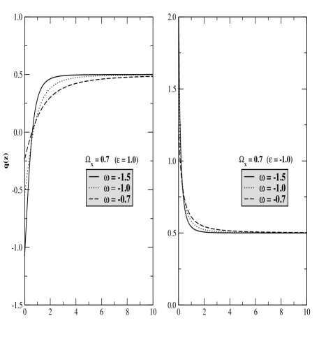
Figure 1: Deceleration parameter as a function of redshift for a fixed value of $\Omega_{x}=0.7$. In both Panels the horizontal line labeled decelerating/accelerating ($q_{o}=0$) divides models with a decelerating or accelerating expansion at a given redshift. Note that while the signature $\varepsilon=1$ gives a speed up scenario at $z_{a}\simeq 1$, the signature $\varepsilon=-1$ implies a slow down scenario

The use of the bulk signature $(4,1)$ associated with $\rho_{extr}>0$ allows us to use the wealth of available data from the recent measurements to determine limits on the values of $\omega^{0}_{extr}$ in our geometric model. For example, from the current SNe Ia data (the so-called gold set of 157 events) one finds $\omega^{0}_{extr}<-0.5$ at 95% confidence level (c.l.) for $\Omega_{\lambda}=\Omega_{k}=0$, regardless of the value of the matter density parameter riess . When combined with Cosmic Microwave Background (CMB) and Large-Scale Structure (LSS) observations, the same SNe Ia data provide $\omega=-1.02^{+0.13}_{0.19}$ (and $\omega<-0.76$ at 95% c.l.) garn . These limits agree with the constraints obtained from a wide variety of different phenomena, using the “cosmic concordance method” wang . In this case, the combined maximum likelihood analysis suggests $\omega^{0}_{extr}\leq-0.6$, (which incidently also rules out an unknown component like topological defects of dimension $n$, such as domain walls and cosmic strings, for which we would have $\omega^{0}_{extr}=-\frac{n}{3}$). Other methods have also contributed to the collection of data. For example, gravitational lens statistics based on the final Cosmic Lens All Sky Survey data suggests that $\omega^{0}_{extr}<-0.55^{+0.18}_{-0.11}$ at 68% c.l. chae ; abha . Similarly, distance estimates of galaxy clusters from interferometric measurements of the Sunyaev-Zel dovich effect and X-ray observations along with SNe Ia and CMB data requires $\omega=-1.2^{+0.11}_{-0.18}$ schu ; alcaniz2003 ; alcaniz2003b . We may also use the measurements of the angular size of high-redshift sources, suggesting that we could take $-1\leq\omega^{0}_{extr}\leq-0.5$ jsa , whereas the use of SNe data and measurements of the position of the acoustic peaks in the CMB spectrum, suggest $-1\leq\omega^{0}_{extr}\leq-0.93$ at 2$\sigma$ cora . We, therefore, conclude that in contrast with the five-dimensional brane-world models with the $\rho^{2}$ term in Friedman’s equation which face experimental constraints, the present geometrical model, at least in the simple case where $\omega^{0}_{extr}$ constant, is consistent with the latest experimental observations, within the limits imposed by the weak energy condition, in the deSitter bulk.

IV Summary

We have provided ample experimental evidence in support to the hypothesis that dark energy can be a consequence of the extrinsic curvature in brane-world cosmology. For that purpose, we have taken the FRW universe, seen as a brane-world embedded in a five dimensional bulk of constant curvature, with undefined signature and the without the $Z_{2}$ symmetry or any form of junction condition. The indefined signature has been motivated mostly by the fact that, except from the theoretical arguments in the application of the AdS/CFT in string theory, there is no experimental argument in favor of the anti-deSitter signature $(3,2)$ over the deSitter signature $(4,1)$.

Under these conditions, Friedman’s equation depends only on the signature of the bulk and on the extrinsic curvature as a possible driver for inflation and. In order to evaluate the compatibility of such geometrical model with the present experimental data, we have established a correspondence with the phenomenological XCDM dark energy model.

In the simple example where the factor $\omega_{extr}$ in the state equation (15) is constant, we found that when the energy density of the geometric fluid is positive and the pressure is negative, the $AdS_{5}$ bulk with signature $(3,2)$ is not compatible with the expected value of the deceleration parameter for the redshift $z\approx 1$, favoring the de Sitter case with signature $(4,1)$. However, if we had taken the expansion energy to be negative, with positive pressure, then the universe would expand in the bulk with signature $(3,2)$.

This example suggests not only that the extrinsic curvature can be the responsible for the accelerated expansion, but also that in the more general case where $\omega_{extr}$ is not constant it mus be dynamic, much in the sense proposed in the literature. The fact that the extrinsic curvature is a symmetric rank-two tensor suggests that the required dynamical equation should be non-linear, in fact an Einstein-like equation Gupta . Work on such ultimate dynamical ”junction” condition is still in progress,

x

Appendix A:
Equations of Motion

With a few exceptions mostly in the five-dimensional cases, the use of differentiable properties of the brane-world embedding have been largely neglected. Nonetheless, the probing of the extra dimensions by gravitons means that the classical geometry of the brane-world should be subjected to continuous deformations (or perturbations) in response to the Einstein-Hilbert dynamics of the bulk. Such deformable embeddings have been studied by Nash and Greene, concluding that the dimension and signature of the bulk is not a matter of choice, but they depend on the the regularity of the embedding functions Nash ; Greene . Therefore, restriction of the bulk to the $AdS_{5}$ geometry requires the use of some additional conditions, like imposing boundary rigidity, and the application of the $Z_{2}$ symmetry. However, it not clear that the full dynamics of the brane-world will be compatible with such limited embedding, except perhaps in some specific cases, as the FRW example in the main text. The embedding is, of course, a fundamental issue in differential geometry which has been frequently applied to general relativity. A comprehensive reference list on space-time embedding properties can be found in Pavsic . In the following we give a short summary on the generation of the differentiable embedding by perturbations of a given background geometry.

Denoting by $\bar{g}_{\alpha\beta}$ the metric of a given four-dimensional manifold $\bar{V}_{4}$ (the background) and by ${\cal G}_{AB}$ the metric of the Riemannian bulk $V_{D}$, the isometric embedding of $\bar{V}_{4}$ is given by a map ${\cal X}:\bar{V}_{4}\rightarrow V_{D}$, with $D=4+N$ components $\bar{\cal X}^{A}$ such that

$$\!\!{\bar{\cal{X}}}^{A}_{,\mu}{\bar{\cal{X}}}^{B}_{,\nu}{\cal G}_{AB}=\bar{g}_{\mu\nu},\;{\bar{\cal{X}}}^{A}_{,\mu}\bar{\eta}^{B}_{b}{\cal G}_{AB}=0,\;\bar{\eta}^{A}_{a}\bar{\eta}^{B}_{b}{\cal G}_{AB}=\bar{g}_{ab}\!\!\!\!$$ (20)

where $\bar{\eta}^{A}_{a}$ are the components of the $N$ independent normal vectors to $\bar{V}_{4}$. According to Nash, we may continuously deform $\bar{V}_{4}$ along a normal direction in the bulk, to obtain another submanifold of the same bulk, provided the embedding functions remain regular (in a generalized sense). Denoting a generic orthogonal direction by ${\eta}=y^{a}\bar{\eta}_{a}$, the deformation (in fact a perturbation) of the embedding can be expressed as

$${\cal Z}^{A}=\bar{\cal{X}}^{A}+(\pounds_{\eta}\bar{\cal{X}})^{A},\;\;\eta^{A}=\bar{\eta}^{A}+(\pounds_{{\eta}}\bar{\eta})^{A}=\bar{\eta}^{A}$$

The components ${\cal Z}^{A}$ and the normal $\eta_{a}$ must satisfy embedding equations similar to (20) (now dependent on $y^{a}$):

$$\phantom{x}\!{\cal Z}^{A}_{,\mu}{\cal Z}^{B}_{,\nu}{\cal G}_{AB}\!\!=\!\!g_{\mu\nu},\;{\cal Z}^{A}_{,\mu}{\eta}^{B}_{a}{\cal G}_{AB}\!\!=\!g_{\mu a},\;\;{\eta}^{A}_{a}{\eta}^{B}_{b}{\cal G}_{AB}\!\!=\!\!g_{ab}\!\!\!\!$$ (21)

From these equations it follows that

$$g^{\mu\nu}Z^{A}_{,\mu}Z^{B}_{,\nu}={\cal G}^{AB}-g^{ab}\eta^{A}_{a}\eta^{B}_{b}$$ (22)

and also the components of the perturbed geometry

$$g_{\mu\nu}(x,y) = {\mathcal{Z}}_{,\mu}^{A}{\mathcal{Z}}_{,\nu}^{B}{\mathcal{G}}_{\!AB}=\bar{g}_{\mu\nu}\!\!-2y^{a}\bar{k}_{\mu\nu a}+$$ (23)

$$y^{a}y^{b}[\bar{g}^{\alpha\beta}\bar{k}_{\mu\alpha a}\bar{k}_{\nu\beta b}+g^{cd}\bar{A}_{\mu ca}\bar{A}_{\nu db}],$$

$$g_{\mu a}(x,y) = {\mathcal{Z}}_{,\mu}^{A}{\eta}_{a}^{B}{\mathcal{G}}_{\!AB}=\!\!y^{b}A_{\mu ab},$$ (24)

$$g_{ab}(x,y) = {\eta}_{a}^{A}{\eta}_{b}^{B}{\mathcal{G}}_{\!AB}=\bar{g_{ab}}$$ (25)

$$k_{\mu\nu a}(x,y) = -\eta_{a,\mu}^{A}{\mathcal{Z}}_{,\nu}^{B}{\mathcal{G}}_{AB}=$$ (26)

$$\phantom{x}\bar{k}_{\mu\nu a}\!\!-y^{b}\bar{g}^{\alpha\beta}\bar{k}_{\mu\alpha a}\bar{k}_{\nu\beta b}-\!\!{g}^{cd}y^{b}\bar{A}_{\mu ca}\bar{A}_{\nu db},\hskip 8.53581pt$$

$$A_{\mu ab}(x,y) = \eta_{a,\mu}^{A}\eta_{b}^{B}{\mathcal{G}}_{AB}\!\!=\!\!\bar{A}_{\mu ab}(x)$$ (27)

From (23) and (26) we obtain York’s relation for the extrinsic curvature (extended to the extra variables $y^{a}$):

$$k_{\mu\nu a}=-\frac{1}{2}\frac{\partial g_{\mu\nu}}{\partial y^{a}}$$ (28)

so that when the brane-world gravitational field represented by the metric $g_{\mu\nu}$ propagates in the bulk, so does the extrinsic curvature.

The components of the Riemann tensor of the bulk written in the the embedding vielbein $\{{\cal Z}^{A}_{,\alpha},\eta^{A}_{a}\}$, give the Gauss, Codazzi and Ricci equations, respectively Eisenhart :

$$\phantom{x}R_{\alpha\beta\gamma\delta}\!\!=\!\!2g^{mn}k_{\alpha[\gamma m}k_{\delta]\beta n}\!\!+{\cal R}_{ABCD}{\cal Z}^{A}_{,\alpha}{\cal Z}^{B}_{,\beta}{\cal Z}^{C}_{,\gamma}{\cal Z}^{D}_{,\delta}$$

$$\phantom{x}k_{\alpha[\gamma b;\delta]}\!\!=\!\!g^{mn}A_{[\gamma mb}k_{\alpha\delta]n}\!\!+{\cal R}_{ABCD}{\cal Z}^{A}_{,\alpha}\eta^{B}_{b}{\cal Z}^{C}_{,\gamma}{\cal Z}^{D}_{,\delta}$$

$$\phantom{x}2A_{[\gamma ab;\delta]}\!=\!\!-2g^{mn}A_{[\gamma ma}A_{\delta]nb}$$

$$- g^{mn}k_{[\gamma ma}k_{\delta]nb}\!\!-{\cal R}_{ABCD}\eta^{A}_{a}\eta^{B}_{b}{\cal Z}^{C}_{,\gamma}{\cal Z}^{D}_{,\delta}$$ (31)

To proceed, we now impose that the bulk geometry is a solution of Einstein’s equations. Denoting $K^{2}=g^{ab}k^{\mu\nu}{}_{a}k_{\mu\nu b}$, $h_{a}=g^{\mu\nu}k_{\mu\nu a}$ and $h^{2}=g^{ab}h_{a}h_{b}$ and using (22), we obtain from the contraction of Gauss’ equations with $g^{\mu\nu}$

$$R_{\mu\nu} = g^{cd}(g^{\alpha\beta}k_{\mu\alpha c}k_{\nu\beta d}-h_{c}k_{\mu\nu d})+{\cal R}_{AB}Z^{A}_{,\mu}Z^{B}_{,\nu}$$ (32)

$$- g^{ab}{\cal R}_{ABCD}\eta^{A}_{a}Z^{B}_{,\mu}Z^{C}_{,\nu}\eta^{D}_{b}$$

A further contraction gives the Ricci scalar

$$R = (K^{2}-h^{2})+{\cal R}-2g^{ab}{\cal R}_{AB}\eta^{A}_{a}\eta^{B}_{b}$$ (33)

$$+ g^{ad}g^{bc}{\cal R}_{ABCD}\eta^{A}_{a}\eta^{B}_{b}\eta^{C}_{c}\eta^{D}_{d}$$

Therefore, the Einstein-Hilbert action for the bulk geometry in $D$-dimensions can be written in terms of the embedded geometry as

$$\int{\cal R}\sqrt{\cal{G}}d^{D}v\equiv\int\left[R-(K^{2}-h^{2})\right]\sqrt{\cal{G}}d^{D}v+$$

$$\phantom{x}\!\!\!\!\!\int\left[2g^{ab}{\cal R}_{AB}\eta^{A}_{a}\eta^{B}_{b}\!\!\!-\!g^{ad}g^{bc}{\cal R}_{ABCD}\eta^{A}_{a}\eta^{B}_{b}\eta^{C}_{c}\eta^{D}_{d}\right]\sqrt{\cal G}d^{D}v$$

$$=\alpha_{*}\int{\cal L}^{*}\sqrt{\cal{G}}d^{D}v$$ (34)

where in the right hand side we have included the bulk source Lagrangian ${\cal L}^{*}$ and we have denoted by $\alpha_{*}$ the D-dimensional fundamental energy scale.

The covariant equations of motion for a brane-world in a D-dimensional bulk can be derived by taking the variation of (34) with respect to $g_{\mu\nu}$, $g_{\mu a}$ and $g_{ab}$, noting that the Lagrangian depends on these variables through ${\cal Z}^{A}_{,\mu}$. Alternatively, wemay just calculate the components of Einstein’s equations for the bulk geometry:

$${\mathcal{R}}_{AB}-\frac{1}{2}{\mathcal{R}}{\mathcal{G}}_{AB}=\alpha_{*}T_{AB}^{*}$$ (35)

in the embedding vielbein $\{{\cal Z}^{A}_{,\alpha},\eta^{B}_{b}\}$. Denoting the vielbein components of the energy-momentum tensor by $T_{\mu\nu}^{*}=T^{*}_{AB}{\cal Z}^{A}_{,\mu}{\cal Z}^{B}_{,\nu}$, $T_{\mu a}^{*}=T^{*}_{AB}{\cal Z}^{A}_{,\mu}\eta^{B}_{a}$ and $T_{ab}^{*}=T^{*}_{AB}\eta^{A}_{a}\eta^{B}_{b}$, we obtain from (35)

$$g^{ab}{\cal R}_{AB}\eta^{A}_{a}\eta^{B}_{b}=\alpha_{*}(g^{ab}T^{*}_{ab}-\frac{N}{N+2}T^{*})$$

From (32) and (33), the (tangent) components of (35) on ${\cal Z}^{A}_{,\mu}{\cal Z}^{B}_{,\nu}$ give the equation for $g_{\mu\nu}$ (sometimes referred to as the gravi-tensor equation)

$$\phantom{x}R_{\mu\nu}-\frac{1}{2}Rg_{\mu\nu}-Q_{\mu\nu}-(W_{\mu\nu}-\frac{1}{2}Wg_{\mu\nu})$$

$$\phantom{x}\hskip 28.45274pt=\alpha_{*}(T^{*}_{\mu\nu}-\frac{N}{N+2}T^{*}g_{\mu\nu}-g^{ab}T^{*}_{ab}),$$ (36)

where we have denoted

$$Q_{\mu\nu}\!\! = \!\!g^{ab}k^{\rho}{}_{\mu a}k_{\rho\nu b}-g^{ab}h_{a}k_{\mu\nu b}\!\!-\!\!\frac{1}{2}(K^{2}-h^{2})g_{\mu\nu}$$ (37)

$$\!\!W_{\mu\nu} = \!\!g^{ad}{\mathcal{R}}_{ABCD}\eta_{a}^{A}{\mathcal{Z}}_{,\mu}^{B}{\mathcal{Z}}_{,\nu}^{C}\eta_{d}^{D}$$

$$W = g^{ad}g^{bc}{\mathcal{R}}_{ABCD}\eta_{a}^{A}\eta_{b}^{B}\eta_{c}^{C}\eta_{d}^{D}$$

On the other hand, again from (35), the trace of Codazzi’s equation (IV) gives the gravi-vector equation

$$\phantom{x}k_{\mu a;\rho}^{\rho}\!-\!h_{a,\mu}\!+\!A_{\rho ca}k^{\rho\;c}_{\;\mu}\!-\!A_{\mu ca}h^{c}\!\!+\!\!2W_{\mu a}$$ (38)

$$\phantom{x}\hskip 22.76219pt=\alpha_{*}(T^{*}_{\mu a}-\frac{1}{N+2}T^{*}g_{\mu a})$$ (39)

where

$$W_{\mu a}=g^{mn}{\cal R}_{ABCD}\eta^{A}_{a}\eta^{B}_{m}{\cal Z}^{C}_{,\mu}\eta^{D}_{n}$$

Finally, the gravi-scalar equation is obtained from (33) and (35)

$$\phantom{x}R-K^{2}+h^{2}-W=-2\alpha_{*}(g^{ab}T^{*}_{ab}-\frac{N+1}{N+2}T^{*})$$ (40)

Equations (36)-(40) represent the most general equations of motion of a brane-world, compatible with the its differentiable embedding in a D-dimensional bulk defined by Einstein’s equations.

The confinement hypothesis as applied to all perturbed geometries (and not just to the background) can be implemented simply as

$$\alpha_{*}T^{*}_{\mu\nu}=-8\pi GT_{\mu\nu},\;\;T^{*}_{\mu a}=0,\;\;T^{*}_{ab}=0$$ (41)

where $T_{\mu\nu}$ denotes the energy-momentum tensor of ordinary matter and gauge fields, which remain confined to the brane-world. As we should expect, (36) reproduces the ordinary Einstein’s equations when the extrinsic geometry components are neglected.

x

Appendix B:
The $Z_{2}$ Symmetry and the Israel-Darmois-Lanczos Condition

Here we use essentially the same procedure as in Israel’s paper Israel , adapted to the case of a brane-world in a constant curvature bulk. The starting point is Einstein’s equation for the bulk geometry (35), now written as

$${\mathcal{R}}_{AB}=\alpha_{*}(T_{AB}^{*}-\frac{1}{2+N}T^{*}g_{AB})$$ (42)

For $D=4+N=5$, the bulk metric written in the embedding vielbein is (just for clarity here we set $g_{55}=\varepsilon=1$)

$${\cal G}_{AB}=\left(\matrix{g_{\mu\nu}&0\cr 0&1}\right)$$

After explicitly writing the vielbein components of the Ricci tensor ${\mathcal{R}}_{AB}$ in the case of the constant curvature bulk, we find from (36) that

$$\phantom{x}\!\!R_{\mu\nu}\!-\!\!\frac{\partial k_{\mu\nu}}{\partial y}\!-\!\!2k_{\mu}^{\rho}k_{\rho\nu}\!\!+\!\!hk_{\mu\nu}\!\!=\!\!\alpha_{*}(T^{*}_{\mu\nu}\!\!-\!\!\frac{1}{3}T^{*}g_{\mu\nu})$$ (43)

Now, consider that the background $y=0$ separates two sides of the bulk, labeled by $+$ and $-$ respectively, and find the value of (43) as we approach $y=0$ from each side.

Like in Israel , we consider two distinct situations: Case (i) is characterized by a continuity of the extrinsic curvature across the boundary $y=0$: $k_{\mu\nu}^{+}=k_{\mu\nu}^{-}$, with the supposition that the confined matter is given by a well defined differentiable energy-momentum tensor. Nothing else is added. Then, in the constant curvature bulk the equations equivalent to the O’Brien-Synge junction conditions (39) and (40), are just identities. As for the tensor equation (36), we notice that the value of $R_{\mu\nu}$ is the same on both sides of $\bar{V}_{4}$. On the other hand, admitting that the brane-world is orientable, then the term $(-\!\frac{\partial k_{\mu\nu}}{\partial y})$ and all terms involving the square of $k_{\mu\nu}$ do not change sign across the boundary. Since in this case the confined matter is intrinsic and well defined, it follows that the differences of (43) calculated on both sides of the boundary cancel each other as $y\rightarrow 0$.

This situation changes in case (ii), characterized by a jump in the extrinsic curvature $k_{\mu\nu}^{+}\neq k_{\mu\nu}^{-}$ across a background caused by a confined distributional source. In this case, the derivatives $(\!\frac{\partial k_{\mu\nu}}{\partial y})$ in (43) continuously changes as it approaches $y=0$, so that the difference between the values of (43) calculated from one to the other side of the background is

$$-[(\frac{\partial k_{\mu\nu}}{\partial y})]=\alpha_{*}\left([T]_{\mu\nu}-\frac{1}{3}[T]g_{\mu\nu}\right)$$ (44)

where we have denoted $[X]=(X^{+}-X^{-})$. Since we cannot anticipate the value of the left hand side of (44) as $y\rightarrow 0$, we may apply the mean value theorem for the differentiable tensor $k_{\mu\nu}$ in the interval $[-y,y]$, to obtain $-[(\!\frac{\partial k_{\mu\nu}}{\partial y})]=\frac{-{k}^{+}_{\mu\nu}+{k}^{-}_{\mu\nu}}{y}$. To evaluate the differences of the right hand sides of (44), we may express $T_{\mu\nu}$ as a delta function, noting that for $X=\bar{X}(x)\delta(y)$ we have

$$y[X]=\int_{-y}^{y}\frac{d}{d\xi}\left(|\xi|{X}\right)d\xi=\int_{-y}^{y}|\xi|\frac{dX}{d\xi}d\xi+\int_{-y}^{y}\frac{\partial|\xi|}{\partial\xi}Xd\xi$$

$$=\int_{-y}^{y}|\xi|\bar{X}\delta^{\prime}(\xi)d\xi+\int_{-y}^{y}\bar{X}\frac{\partial|\xi|}{\partial\xi}\delta(\xi)d\xi=2\bar{X}$$

In particular, for $\bar{X}=(\bar{T}_{\mu\nu}-1/3\bar{T}\bar{g}_{\mu\nu})$, we obtain Lanczos’ equation describing the jump of the extrinsic curvature

$${k}_{\mu\nu}^{+}-{k}_{\mu\nu}^{-}=-2\alpha_{*}(\bar{T}_{\mu\nu}-\frac{1}{3}\bar{T}\bar{g}_{\mu\nu})$$ (45)

To obtain the IDL condition we need to specify how $k_{\mu\nu}$ changes from one side to the other. This is precisely what the $Z_{2}$ symmetry does, where the background $y=0$ acts as a mirror for all objects that sense the extra dimension. The normal $\eta_{,\mu}$ and its derivatives have inverted mirror images, so that from the definition (26), the jump of the extrinsic curvature is

$$k^{+}_{\mu\nu}=-k^{-}_{\mu\nu}$$ (46)

so that equation (45) gives at $y=0$ the Israel-Darmois-Lanczos condition

$$\bar{k}_{\mu\nu}=-\alpha_{*}(\bar{T}_{\mu\nu}-\frac{1}{3}\bar{T}\bar{g}_{\mu\nu})$$ (47)

specifying the value of the extrinsic curvature of the background in terms of the energy-momentum tensor of its confined sources.

Reciprocally, using the definition of $k_{\mu\nu}$, the values calculated on the two sides of the background are $k_{\mu\nu}^{\pm}=-{\cal Z}_{,\mu}^{A}\eta^{\pm B}_{\;\;,\nu}\,{\cal G}_{AB}$, and therefore (46) implies that $\eta^{A+}_{,\mu}=-\eta^{A-}_{,\mu}$, or in other words that the background behaves as a mirror for the derivatives of $\eta$. We conclude that while (45) follows from Einstein’s equation of the bulk plus the distributional source of the brane-world, the $Z_{2}$ symmetry (or any symmetry producing the same mirror effect) completely specifies $\bar{k}_{\mu\nu}$ in terms of the confined source $\bar{T}_{\mu\nu}$.

One aspect that has not been considered is that the IDL condition, which was originally applied to two or three dimensional hypersurfaces, may imply in a limited class of admissible background brane-worlds in a higher-dimensional bulk, depending on how general is that confined source. For example, if we consider a confined source such as $\bar{T}_{\mu\nu}=1/3\bar{T}\bar{g}_{\mu\nu}$, then from (47) it follows that $\bar{k}_{\mu\nu}=0$ which means that the background is just a plane. But from (26) it follows that all perturbations also have zero extrinsic curvatures and consequently they are also planes. Some other examples are discussed in Szekeres ; Collinson

Another mathematical aspect which deserves further attention is the fact that with the $Z_{2}$ symmetry, for each perturbation of the background there will be a mirror image on the other side of it. Therefore, to each point of the background corresponds two different tangent vectors, one on each side, whose projections on the background give vectors pointing on opposite directions. This means that the derivatives of the embedding functions are not well defined. Under this condition the perturbations of the background cannot be guaranteed to remain an embedded differentiable manifold Nash .

References

- (1) S. Perlmutter et al., Astrophys. J. , 517, 565, (1999); A. Rises et all, Astron. J. 116, 1009 (1998).
- (2) S. Weinberg, Rev. Mod. Phys. 61, 1, (1989); S. Weinberg, astro-ph/9610044.
- (3) N. Strumann, proc. Heidelberg 2000, 110-124, (2000), astro-ph/0009386.
- (4) R. Caldwell, et al, Phys. Rev. Let. 80, 1582 (1998).
- (5) S. M. Carroll, astro-ph/0107571.
- (6) M. S. Turner and M. White, Phys. Rev. D56, R4439 (1997); T. Chiba, N. Sugiyama and T. Nakamura, Mon. Not. Roy. Astron. Soc., 289, L5 (1997); J. S. Alcaniz and J. A. S. Lima, Astrophys. J. , 550, L133 (2001) (astro-ph/0109047); Z.-H. Zhu, M.-K. Fujimoto and D. Tatum, Astron. Atrophys. 372, 377 (2001); A. R. Cooray & D. Huterer, Astrophys. J. 513, l95 (1999); P. S. Corasaniti et al, Phys. Rev. D70, 083006 (2004); Y.Wang & M. Tegmark, Phys. Rev. Lett. 92, 241302-1 (2004)
- (7) N. Arkani-Hamed et Al, Phys. Lett. B429, 263 (1998), Phys. Rev. Lett. 84, 586, (2000).
- (8) L. Randall & R. Sundrum, Phys. Rev. Lett. 83, 3370,(1999); L. Randall and R. Sundrum, Phys. Rev. Lett. 83, 4690 (1999).
- (9) R. Maartens, Living Rev.Rel.7:1-99,2004, gr-qc/0312059.
- (10) D. Langlois, gr-qc/0410129
- (11) Eun-Joo Ahnn, Maximo Ave, Marco Cavaglia, Angela V. Olinto, Phys. Rev. D68, 043004,(2003), hep-ph/0306008, also, Phys.Lett. B551,1, (2003), hep-th/0201042
- (12) S. Dimopoulos & G. Landsberg, hep-ph/0106295
- (13) K. Cheung, DPF annual meeting, APS, (2003), hep-ph/0305003
- (14) M. Cavaglia, S. Das and R. Maartens, Class. Quant. Grav. 20, L205 (2003).
- (15) A. Pérez-Lorenzana, Mexican School on Particle and Fields, Metepec 2000, 53-85 (2000), hep-ph/0008333.
- (16) P. Binetruy, C. Deffayet and D. Langlois, Nucl. Phys. B565, 269, (2000). hep-th/9905012.
- (17) P. Binetruy et al, Phys. Lett. B477, 285 (2000), hep-th/9910219.
- (18) J. M. Cline et al, Phys. Rev. Lett. 83, 4245 (1999).
- (19) S. Tsujikawa & A. R. Liddle, ICAP, 0403, 001, (2004), astro-ph/0312162.
- (20) M. D. Maia, astro-ph/0404370
- (21) S. Tsujikawa, M. Sami & R. Maartens, Phys. Rev. D70, 063525, (2004), astro-ph/0406078
- (22) J. D. Bratt et al, Phys. Lett.D70, 063525, (2004)
- (23) C. Ringeval, T. Boehm, R. Durrer hep-th/0307100.
- (24) G. Dvali, G. Gabadadze & M. Porrati, Phys. Lett. B485, 208 (2000)hep-th/0005016.
- (25) G. Dvali & M. S. Turner, astro-ph/0301510
- (26) M. D. Maia et al, Int.J.Mod.Phys A17, 4355, (2002), gr-qc/0212059
- (27) Anne-Christine Davis et all, Phys. lett. B504, 254, (2001), hep-ph/0008132
- (28) L.A.Gergely, Phys. Rev. D68, 124011 (2003), gr-qc/0308072
- (29) P. Bowcock, C. Charmosis & R. Gregory, Class. Quant. Grav. 17, 4745, (2000), hep-th/0007177
- (30) B. Carter & J. P. Uzan, Nucl. Phys. B606, 45, (2001), gr-qc/0101010
- (31) N. Deruelle, T. Dolezel and J. Katz, Phys. Rev. D63, 083513 (2001) hep-th/0010215.
- (32) R. A. Battye & B. Carter, Phys. Lett. B509, 331, (2001), hep-th/0101061.
- (33) R. A. Battye et al, Phys. Rev. D64, 124007, (2001).
- (34) M. D. Maia & E. M. Monte, Phys. Lett. A297, 9 (2002).
- (35) M. D. Maia, E. M. Monte, J. M. F. Maia , Phys.Lett. B585, 11, (2004), astro-ph/0208223.
- (36) J. Nash, Ann. Maths. 63, 20, (1956).
- (37) R. Greene, Mem. Amer. Math. Soc. 97 (1970).
- (38) K. Maeda, Phys. Rev. D64, 123525 (2001). astro-ph/0012313.
- (39) J. Rosen. Rev. Mod. Phys. 37, 204, (1965).
- (40) M. D. Maia & W. L. Roque Phys. Lett. A139. 121, (1989).
- (41) V. Sahni & Y. Shtanov, JCAP, 0311, 014, (2003), astro-ph/0202346,
- (42) M. S. Turner & A. G. Riess, Astrophys. J. 569, 18 (2002).
- (43) M. S. Turner & A. G. Riess, Astrophys. J. 607, 665 (2004).
- (44) P. M. Garnavich et al., Astrophys. J. 509, 74 (1998).
- (45) L. Wang et al Astrophys. J. 530, 17 (2000).
- (46) Kyu-Hyun Chae et al., Phys. Rev. Lett. 89, 151301 (2002).
- (47) A. Dev, D. Jain & S. Mahajan, Intl. J. Mod. Phys. D13, 1005, (2004), astro-ph/0307441.
- (48) P. Schuecker et al, Astron-Astrophys. 402, 53 (2003), astro-ph/0211480.
- (49) J. S. Alcaniz, Phys. Rev. D69, 083521 (2004), astro-ph/0312424.
- (50) J. S. Alcaniz, Phys. Rev. D69, 083521 (2004)
- (51) J. A. S. Lima & J. S. Alcaniz, Astrophys. J. 566, 15 (2002).
- (52) P. S. Corasaniti & E. J. Copeland, Phys. Rev. D65, 043004 (2002).
- (53) S. N. Gupta, Phys. Rev. 96, 1683, (1954).
- (54) M. Pavsic and V. Tapia, gr-qc/0010045.
- (55) L. P. Eisenhart, Riemannian Geometry, Princeton U.P. Reprint (1966).
- (56) W. Israel, Il Nuovo Cimento, 44, 4349, (1966).
- (57) P. Szekeres, Il Nuovo Cimento, 43, 1062 (1966)
- (58) C. D. Collinson, J. Phys. A 4, 206 (1971)