Hyperfine Structure in H¹³CO⁺ and ¹³CO: measurement, analysis, and consequences for the study of dark clouds

The magnetic moment of the ¹³C nucleus is shown to provide a potentially useful tool for analysing quiescent cold molecular clouds. We report discovery of hyperfine structure in the lowest rotational transition of H¹³CO⁺. The doublet splitting in H¹³CO⁺, observed to be of width 38.5$\pm$5.2 kHz or 0.133 km s^-1, is confirmed by quantum chemical calculations which give a separation of 39.8 kHz and line strength ratio 3:1 when H and ¹³C nuclear spin-rotation and spin-spin coupling between both nuclei are taken into account. We improve the spectroscopic constants of H¹³CO⁺ and determine the hitherto uncertain frequencies of its low-$J$ spectrum to better precision by analysing the dark cloud L 1512. Attention is drawn to potentially high optical depths (3 to 5 in L 1512) in quiescent clouds, and examples are given for the need to consider the (1 – 0) line’s doublet nature when comparing to other molecular species, redirecting or reversing conclusions arrived at previously by single-component interpretations.
We further confirm the hyperfine splitting in the (1 – 0) rotational transition of ¹³CO that had already been theoretically predicted, and measured in the laboratory, to be of width about 46 kHz or, again, 0.13 km s^-1. By applying hyperfine analysis to the extensive data set of the first IRAM key-project we show that ¹³CO optical depths can as for H¹³CO⁺ be estimated in narrow linewidth regions without recourse to other transitions nor to assumptions on beam filling factors, and linewidth and velocity determinations can be improved. Thus, for the core of L 1512 we find an inverse proportionality between linewidth and column density, resp. linewidth and square root of optical depth, and a systematic inside-out increase of excitation temperature and of the ¹³CO:C¹⁸O abundance ratio. Overall motion toward the innermost region is suggested.

1 Introduction

It has long been recognised that cold interstellar clouds are excellent laboratories for determining basic physical quantities of molecular structure. These clouds also provide the only access to molecular species that are too unstable to permit sufficient terrestrial production for in-depth investigation. A good case in point here is the X-ogen of the early 1970s, alias oxomethylium or the formyl cation, HCO⁺ (e.g. Snyder et al. 1976) which has since gained prime importance for studying the interactions between interstellar gas and magnetic fields.

In some of these clouds, microwave emission profiles are so narrow that line frequencies can be determined to between seven and eight significant digits, relative to other lines, corresponding to an accuracy of some ten meters per second in velocity, or Mach 0.02 at typical temperatures. A recent example is the re-analysis of the N₂H⁺(1 – 0) transitions (Caselli et al. 1995) which led to a frequency determination with precision 7 kHz, difficult to attain with laboratory spectroscopy. It thus becomes possible to study minute motions in such objects that may be on the brink of collapsing toward star formation.

With this aim we have observed the dark cloud Lynds 1512 in numerous molecular transitions. This object is a small accumulation of opaque blobs on the POSS plates, situated near the edge of the Taurus-Auriga-Perseus complex. Ever since Myers & Benson (1983) discovered ammonia radiation from one of these blobs, this “core” has been known as a source of particularly narrow emission lines and has consequently attracted much attention, among many others that of Fiebig (1990) who from NH₃ observations derived a kinetic temperature of 9.7 K at the center, Muders (1995) who drew attention to the cloud’s well-structured velocity field, and more recently from the extensive IRAM Key Project on pre-star-forming regions (Falgarone et al. 1998).

Somewhat to the East of the L 1512 ammonia peak there exists a region particularly well-suited for high-precision line studies because there, several tracers of high gas density like CCS, HC₃N and C₄H show very narrow emission profiles whose widths indicate the kinetic temperatures of the gas to be not more than 9 to 10 K. There is a certain velocity gradient all over L 1512 which must be subtracted off when determining intrinsic linewidths, but many coexisting species are subject to this same gradient and can therefore be compared to each other very well over the whole region. Their intrinsic profiles then turn out to be basically identical.

There is one high-density tracer however which does not at all fit this general picture of uniformity: H¹³CO⁺. We found its linewidth to be considerably broader than that of the other species, and its profiles to be non-Gaussian all over this region. Since HCO⁺, being tied by its electric charge to collapse-retarding magnetic field lines, could be the prime informer on the interaction between neutral and charged molecules in dynamic clouds, it seemed important to clarify the reason for this difference. We thus realised that the magnetic moment of the ¹³C nucleus – in conjunction with the much less efficient moment of the single proton – might cause an observable hyperfine splitting in the H¹³CO⁺(1 – 0) line, of sufficient separation to be developed into a useful tool for spectral analysis. Subsequently we searched for a similar splitting in the (1 – 0) line of the low-density tracer molecule ¹³CO as well. Below we will report on some possibilities for line interpretation that emerge from the fact that again the splitting is wide enough to be observed in quiescent cold clouds.

This paper is organised as follows. In section 2 we summarise the observations performed at various telescopes, then present some general results in section 3. Section 4 discusses the observed H¹³CO⁺(1 – 0) line shapes, the determination of the width of the hyperfine splitting, and the ensuing high optical depths of this isotopomer. In section 5 our quantum chemical calculations concerning the hyperfine structure of this molecule are reported and improved spectroscopic constants derived. Line frequencies for the low-$J$ rotational spectra of H¹³CO⁺ (and HC¹⁸O⁺) can then be determined with high precision in section 6. Some examples of the analytical possibilities provided by the seeming complication due to hyperfine structure are given in section 7. Section 8 investigates the corresponding splitting for the ¹³CO molecule, which allows several physical trends to be established for the core of L 1512. Finally, section 9 presents our conclusions.

2 Observations

2.1 IRAM 30m Observations

Our H¹³CO⁺(1 – 0) and HC₃N(10 – 9) data were taken simultaneously with the IRAM 30-meter telescope on Pico Veleta during several sessions between November 2000 and the summer of 2001. We used one of the 3mm SIS facility receivers. At the line frequency of 86.754 GHz the single sideband receiver noise temperature was $\sim$60 K and the FWHM beam size 29^′′. The spectra were analysed with the autocorrelator at 10 kHz (i.e. 0.034 km s^-1) resolution. We checked the pointing accuracy regularly on nearby continuum sources. It was better than 2^′′.

The data were observed using the frequency switching technique with a shift of $\pm$1 MHz, which is large enough to separate the very narrow lines and small enough to get a very good baseline. The spectra were scaled to the main beam brightness temperature scale using the efficiencies supplied by the observatory ($\eta_{\rm mb}=0.78,\eta_{\rm ff}=0.92$). Throughout the sessions the average system noise temperatures including the atmosphere were $\sim$170 K (main beam scale) which corresponds to an atmospheric opacity of about 0.1.

2.2 HHT Observations

The HCO⁺(3 – 2) data were measured with the 10-meter Heinrich Hertz Telescope (HHT) on Mt. Graham, AZ in February 1999 and March 2000. The facility 1mm SIS receiver operated in double sideband mode and had a receiver noise temperature of $\sim$170 K. We used the 62.5 kHz resolution filterbank to analyse the spectra.

At the line frequency of 267.558 GHz, the FWHM beam size was 32^′′. The main beam efficiency was 0.78 and the forward efficiency 0.95. The pointing accuracy, from measurements of planets and other strong continuum sources, was better than 3^′′.

In February 1999 the observing conditions were good and stable throughout the entire observing period with average DSB system temperatures of $\sim 500$ K (main beam scale), corresponding to atmospheric opacities of $\sim 0.2$. The conditions in March 2000 were worse, with average system temperatures of $\sim 900$ K and opacities of $\sim 0.4$.

We used the On-The-Fly mapping method to obtain fully sampled maps of the HCO⁺(3 – 2) emission toward L 1512.

2.3 Effelsberg 100m Observations

The 30 GHz cooled HEMT receiver on the MPIfR 100-m telescope was used between January 1997 and March 1999 for mapping the HC₃N(3 – 2) triplet as well as transitions of some other species (see Fig. 2) in L 1512. At the line frequency of 27.294 GHz the FWHM beam size was 33^′′ and the receiver noise temperature $\sim 65$ K. We employed the facility autocorrelators at a resolution of 1.5 and 2.5 kHz (0.015 and 0.025 km s^-1), taking special care to keep the velocity calibration always consistent. On-The-Fly mapping was done in frequency-switching mode at a throw of $\pm$0.4 MHz.

The NH₃(1,1) emission at 23.694 GHz was measured repeatedly, using the old Effelsberg 1.3 cm K-band as well as the new 1.3 cm HEMT receiver. The FWHM beam size at that frequency is 39.6^′′. The receiver noise temperatures were typically of order 50 K; main beam efficiency here is 58 percent. We mostly used spectral resolutions of 1.25 or 2.5 kHz which correspond to 0.016 resp. 0.032 km s^-1, and observed in frequency-switching mode of throw $\pm$0.14 MHz.

2.4 The ¹³CO(1 – 0) and C¹⁸O(1 - 0) Spectra

Apart from a few C¹⁸O(1 – 0) spectra that were taken simultaneously with our H¹³CO⁺(1 – 0) measurements mentioned above, all CO data used in this paper come from the IRAM Key Project (IKP) on small-scale structure of pre-star-forming regions whose observational conditions have been fully reported by Falgarone et al. (1998) and will not be repeated here.

3 Results

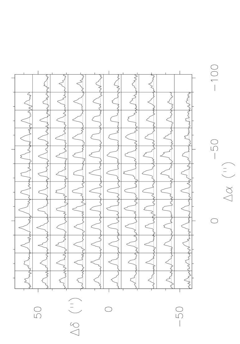
Figure 1: Grid of H¹³CO⁺(1 – 0) emission profiles from L 1512. T_mb (from -0.3 to 1.5 K) is shown as function of v_LSR (from 6.5 to 7.8 km s^-1). Offsets are relative to RA(1950) 05 00 54.4, Dec (1950) 32 39 00.

Our map of H¹³CO⁺(1 – 0) profiles is displayed in Fig. 1 where coordinate offsets are counted from the position RA(1950) 05 00 54.4, Dec (1950) 32 39 00. Note that the true NH₃ and N₂H⁺ peaks (i.e. the cloud’s core center) are at the approximate offset (-25^′′,10^′′).

Sizeable radiation extends somewhat further out than that of the other carbon-containing high density tracers mentioned in the introduction. In contrast to these tracers H¹³CO⁺(1 – 0) does not show any brightness decline around the true ammonia peak that would signal molecular depletion in the innermost region due to freeze-out onto grains. This poses a problem. Absence of a noticeable depletion dip is verified by the recently published H¹³CO⁺(1 – 0) map of Hirota et al. (2003) which at a velocity resolution of 0.13 km s^-1 covers the same area as ours plus an extension to the North where emission is seen far beyond that from, e.g., HC₃N.

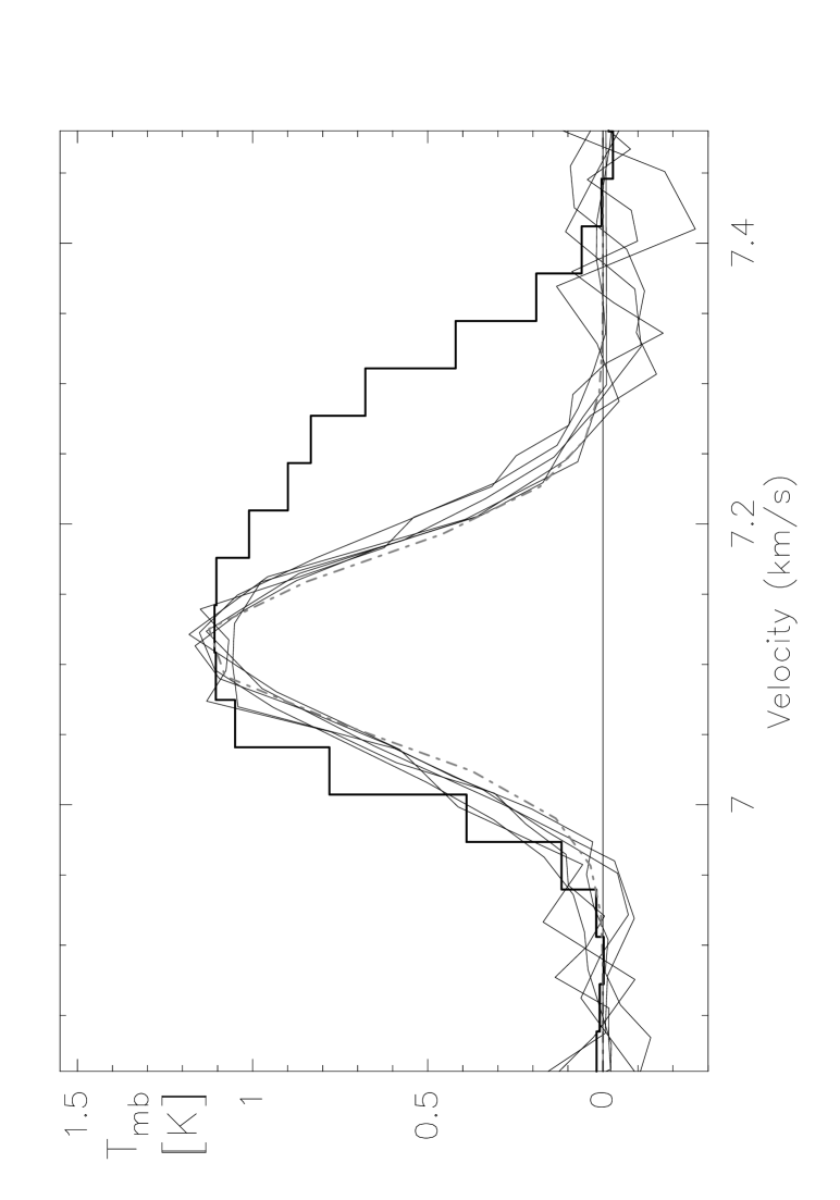
Figure 2: Line profiles of H¹³CO⁺(1 – 0) (histogram), NH₃(1,1:L1), C¹⁸O(1 – 0), C₄H(3 – 2:J–7/2–5/2 F=4–3 and 5/2–3/2 F=2 – 1), HC₃N(3 – 2, F=2 – 1) and CCS(3 – 2), all taken at offset (0^′′, -9^′′) and frequency-shifted for optimal overlap. The dash-dotted curve is the reduced H¹³CO⁺(1 – 0) profile. Scales are for H¹³CO⁺(1 – 0); rescaling for the other species as described in the text.

Both widths and shapes of our H¹³CO⁺(1 – 0) profiles differ noticeably from those of other coexisting trace species. Typical FWHM widths in Fig. 1 are around 0.28 km s^-1, with a slight increase near offset (-60^′′, -10^′′) which is, however, less marked than for numerous other molecules. A sample spectrum, taken in long integration at offset (0^′′, -9^′′), i.e. about halfway between the center and the edge of the high-density core of L 1512, is shown in Fig. 2 together with low-transition profiles of other coexisting species, namely NH₃, C¹⁸O, C₄H, HC₃N and CCS, all from the same position. The frequencies of these species here have been shifted and their amplitudes normalised for better comparison; furthermore, each species’ velocity scale has been expanded or compressed with the square root of the mass ratio between the molecule in question and H¹³CO⁺. In this way it becomes evident that, at this position, their true linewidths go with (molecular mass)^-1/2; if all these species had atomic weight 30 amu, each line would be between 0.15 and 0.16 km s^-1 wide. This value would have to be reduced for several reasons like nonzero optical depth (typically a few to 15 percent reduction), velocity gradient in the beam (a few percent for the velocity field of L 1512) plus likely also one along the line of sight, binning and folding of frequency-switched lines (another 5 percent), in order to obtain the intrinsic width. The purely thermal value for 10 K would be 0.126 km s^-1. Hence the gas is very cold and quiescent even though its position is not at the core’s center where the lowest temperatures are believed to exist. There is no indication of macroscopic motion in any of the line shapes with the possible exception of that of H¹³CO⁺.

The asymmetry of the stepped profile of Fig. 2 is not seen in any other comparable molecule in this source. It is not confined to a limited location. At the majority of positions in Fig. 1 the lines have a steeper slope on the left than on the right, never the other way round; the higher-velocity side often appears somewhat “bumpy”. This singular feature will be discussed next.

4 Interpretation of H¹³CO⁺(1 – 0) line shapes in L 1512

Line asymmetries can be caused by several mechanisms, like a sufficiently large velocity gradient within the cloud, superposition of several emitters along the line of sight, or (self)absorption by cooler gas on the near side of the source. For the core of L 1512 several other species suggest that in low-lying transitions neither of these mechanisms is generally at work. Since this core is known to exhibit very strong self-absorption in the HCO⁺(3 – 2) transition, however (cf Fig. 4b), it would not be surprising to find the third mechanism relevant in H¹³CO⁺(1 – 0). Unfortunately, the frequency of H¹³CO⁺(1 – 0) was not known a priori with high enough precision to let comparison with other lines decide the question of foreground absorption. The absorption trough in the main isotopomer’s (3 – 2) transition clearly shifts across the line with position on the sky while the H¹³CO⁺ bump is static: any hypothetical foreground absorbers of H¹³CO⁺(1 – 0) should thus be fixed locally to the emitters in velocity space, a somewhat special situation. For these reasons we were led to suspect a hyperfine splitting (hfs) as the cause of the relatively large linewidths and asymmetry.

4.1 Observation of the Hyperfine Splitting

Figure 3: Best-fit separations of the primary and secondary components of the H¹³CO⁺(1 – 0) hyperfine doublet for all independent measurements, as a function of the measurement’s signal-to-noise ratio. S is mean intensity over the line, N the noise at spectral resolution 0.0337 km s^-1. Horizontal lines give the mean value and rms error.

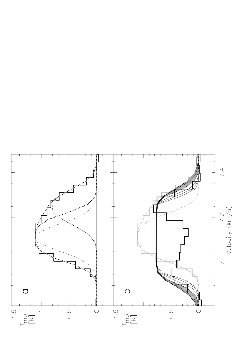
Figure 4: a) Deep integration H¹³CO⁺(1 – 0) spectrum (histogram) from offset (0^′′, -9^′′), and its resolution into primary and secondary hyperfine components (dots) which combine into the dashed profile. The dash-dot curve is the intrinsic primary profile (i.e. before widening by optical depth). b) H¹²CO⁺(3 – 2) spectrum (dark histogram) from the same position, compared to what would be expected when extrapolating, under simplifying assumptions, from the H¹³CO⁺(1 – 0) observation. Depending on the latter’s assumed total peak optical depth $\tau_{13}$, here 0.1, 1, 2, 3, 4, 5, the smooth flat-topped profiles would be expected for H¹²CO⁺(3 – 2). Grey area: $\tau_{13}$ below 2; inner three full lines: $\tau_{13}$ = 3, 4, 5.

The magnetic moments of proton and ¹³C nucleus must in principle lead to such a splitting, of unknown width. Therefore we reduced each profile, in the $60^{\prime\prime}\times 110^{\prime\prime}$ field centered on $(0^{\prime\prime},\leavevmode\nobreak\ 0^{\prime\prime})$ which contains the sources of narrowest line emission in the whole cloud, by a set of assumed values of the splitting width, keeping the line strength ratio fixed at 3:1 as prescribed by basic quantum theory (see section 5), and chose that value which optimally fits the measurement to be the profile’s most likely value. All of these most likely values together are shown in Fig. 3; their consistency leaves little doubt that the width of the splitting can well be determined in this region of exceptional immobility and low temperature, and rules out self-absorption as an essential feature.

The mean value of the hyperfine splitting so determined emerges as 0.133 km s^-1 or 38.5 kHz, with a rms deviation of 0.018 km s^-1. Since there are some 20 independent measurements contained in the data of Fig. 3, the error might be considerably smaller still but, at these levels, systematic errors may come into play.

With this result, and a line strength ratio of 3:1 (high:low frequency) as given by theory (see below), we can resolve the H¹³CO⁺(1 – 0) profile of Fig. 2 into the two components depicted in Fig. 4a by the dotted lines. Total optical depth, $\tau_{13}$, at this particular position is determined by comparing these components: it is between around 3 and 5. Hence the stronger component must be considerably wider than the profiles of the other molecular species shown in Fig. 2 whose $\tau$ is typically at or below unity. The reduced width (i.e. after correction for optical depth) of this H¹³CO⁺(1 – 0) profile turns out to be 0.138 $\pm$ 0.006 km s^-1, however, in agreement with the others’ values mentioned above. From $\tau_{13}$ and T_mb the excitation temperature of the line follows as between 3.9 and 4.6 K, uncertain mainly because of uncertain calibration.

4.2 Large optical depths of H¹³CO⁺ ?

Before turning to theoretical calculations of the multiplet structure we make some comments on this seemingly very high value of optical depth. If confirmed, this could explain the seeming absence of central depletion that was mentioned above. Virtually most published observations of H¹³CO⁺(1 – 0) to date have been interpreted under the assumption of the line being optically thin, with typical $\tau$ values around 0.1 to 0.4, although observed radiation temperatures would then often require a questionably high excitation of the molecule. As will be discussed below, the C¹⁸O(1 – 0) emission from the position of Fig. 2 has an optical depth at line center of 0.72 and CO excitation temperature 9 K. We can then ask what the corresponding optical depth of our H¹³CO⁺ line should be in case the standard abundance ratios for ¹²CO:H¹²CO⁺ of $1.0\times 10^{4}$ for dark clouds (Irvine et al. 1987) and $\approx 7$ for ¹³CO:C¹⁸O were applicable in the present context. With the two excitation temperatures given above, we calculate 44 percent of all C¹⁸O molecules (in LTE), and about the same percentage of all H¹³CO⁺ (not in LTE) to be in state $J$=1. The $\tau({\rm H^{13}CO^{+}}):\tau({\rm C^{18}O})$ ratio then is 2.24$\times 7\times 10^{-4}\times(\mu({\rm H^{13}CO^{+}}):\mu({\rm C^{18}O}))^{2}$, where the factor 2.24 contains all the statistics (and whose narrow error margin of 10 to 15 percent is hardly negotiable); $\mu$ is the electric dipole moment of the species in question. The $\mu$ quotient is $\approx$ 35 if $\mu({\rm H^{13}CO^{+}})$ = 3.93 D (Botschwina et al. 1993) is assumed; it could be somewhat higher.

In this way we deduce the H¹³CO⁺ line’s optical depth to be about twice that of C¹⁸O, or 1.5 at the present position, a value by no means negligible and quite compatible with the 3 to 5 derived above considering the several uncertainties involved. The most insecure factor would seem to be the CO:HCO⁺ ratio, a reduction of which by fifty percent could bring our estimates nicely in line.

Further support for high H¹³CO⁺ optical depths comes from a somewhat simplistic comparison to the main isotopomer’s (3 – 2) emission from the same position on the sky (the dark histogram in Fig. 4b). The lower $\tau_{13}$, the higher the intrinsic linewidth must be to fit the H¹³CO⁺ profile. This means higher H¹²CO⁺ linewidth as well, so that a certain $\tau_{13}$ limit is given by the measured H¹²CO⁺ width. It is assumed here that both profiles originate from physically similar gas. If both isotopomers had T_ex values around 9 K, $\tau_{13}$ would have to be at least 0.17 to produce the amplitude of the spectrum of Fig. 2. Hence the optical depth of H¹²CO⁺(3 – 2) would be some 1.24$\times$abundance ratio, or $\approx$ 50 to 90 times as high, i.e. around 10 to 15. Combined with the required intrinsic linewidth this results in a minimum width of the H¹²CO⁺ profile that is considerably wider than what is observed. How would this change in the case of non-LTE? Under the two natural assumptions that excitation temperatures T_ex for the rarer isotopomer are not higher than for the dominant one (because radiative excitation will push the optically deeper species closer to LTE), and that T_ex does not increase with increasing rotational transition, it is straightforward to determine lower limits on the $\tau_{12}:\tau_{13}$ ratio independent of the degree of deviation from LTE. For each assumed value of $\tau_{13}$ and its corresponding intrinsic linewidth, a minimum width of the H¹²CO⁺ profile can thus be computed. Examples for various $\tau_{13}$ are given in Fig. 4b as the smooth and dotted dark curves, using a ¹²CO:¹³CO abundance ratio of 70 for demonstration. As $\tau_{13}$ is increased, the computed H¹²CO⁺ profiles contract. The grey-shaded region covers $\tau_{13}$ from 0.1 to 1 to 2 (dots); the full lines correspond to $\tau_{13}$ = 3, 4, and 5 (the innermost one).

It seems that $\tau_{13}$ values below about 2 would require too wide an H¹²CO⁺ line. Due to the strong selfabsorption of that line the argument depends somewhat on its true (unabsorbed) value of T_mb. From comparison with the other positions in the map (where selfabsorption shifts widely across the line), T_mb values below 0.75 K are improbable. 0.75 K means T_ex(H¹²CO⁺(3 – 2)) equal to 4.60 K. Note that nearly all across the map H¹²CO⁺ widths are too narrow to allow $\tau_{13}$ values much below about 2.

Since the width of a double-structure profile may considerably exceed the intrinsic linewidth, the usual formulae for column density have to be reconsidered. If the molecules have a Gaussian distribution in velocity space, with the full width at half maximum equal to $\Delta v$, the general expression for the column density of the ground state, $N_{0}$, is, independent of hyperfine multiplicity and for arbitrary optical depths,

$$N_{0}=c_{0}\cdot(\nu_{10}/c)^{3}\cdot A_{10}^{-1}\cdot f_{bf}\cdot(1-e^{-T_{0}/T_{ex}})^{-1}\cdot\tau_{13}\cdot\Delta v$$

where $c_{0}=\frac{4}{3}(\pi^{3}/{\rm ln}(2))^{1/2}$, $\tau_{13}$ the total peak optical depth, i.e. the sum of the two components, $A_{10}$ the Einstein coefficient for the 1 – 0 transition, $\nu_{10}$ the line frequency, T${}_{0}=h\nu_{10}/k$ = 4.16 K, T_ex the excitation temperature between states 1 and 0, and $f_{bf}$ the beam filling factor. $\Delta v$ is the intrinsic linewidth of either component, before broadening by optical depth, and not the observed profile width. $A_{10}$ is $3.9\times 10^{-5}\cdot(\mu/3.93\;D)^{2}\;{\rm s}^{-1}$, hence

$$N_{0}=5.50\times 10^{11}\cdot\tau_{13}\cdot\Delta v\cdot(1-e^{-T_{0}/T_{ex}})^{-1}{\rm cm}^{-2}$$

if $\mu$ = 3.93 D and $f_{bf}$ = 1 is assumed and $\Delta v$ is measured in km s^-1.

To translate this ground-state into total column density, the partition function is required. In the present case, where T_ex is around 4 to 4.6 K, this can be obtained quite reliably since levels above $J$=1 are hardly occupied, contributing altogether less than 20 percent to the partition function. That function is then 2.5 to within less than 15 percent uncertainty, so that the total H¹³CO⁺ column density at the position of Fig. 2 becomes $1.2\times 10^{12}$ cm^-2 for the T_ex, $\tau_{13}$, and $\Delta v$ values derived above.

5 Hyperfine structure in H¹³CO⁺ and related species

The presence of one or more nuclei with spins of $I\geq 1$ causes a rotational transition to appear as a group of several components due to interactions between the electric quadrupole moments of these nuclei and the electric field gradients present around them. The splitting between the lines is frequently resolved in laboratory spectroscopy, and to some extent even in astronomical observations, in particular for transitions with low values of $J$.

It is less well known that for molecules with one or more nuclei having $I\geq 1/2$ there exists another hyperfine effect: the coupling of the nuclear magnetic spin to rotation. While in the case of nuclei with $I\geq 1$ this effect results only in a shift of the quadrupole components, it causes each rotational level with $J>0$ to split into two for nuclei with $I=1/2$. In the laboratory, the nuclear spin-rotation splitting due to a nucleus with $I=1/2$ is generally not resolvable by Doppler-limited rotational spectroscopy. Sub-Doppler methods, such as Lamb-dip spectroscopy or microwave Fourier transform spectroscopy, may overcome this obstacle.

The nuclear spin-rotation coupling constants, $C$, describing this effect are proportional to the rotational constants, to the magnetic moments and to the inverse of the spin-multiplicity $2I+1$ of the nuclei. In addition, the presence of low-lying electronic states causes the magnitude of the $C$s to increase in a complex way.

The nuclear spin-rotation coupling constants for H¹³CO⁺ have not yet been determined experimentally. Therefore, quantum chemical calculations were performed at the ETH Zürich in order to evaluate the nuclear spin-rotation coupling constants of several isotopomers of HCO⁺. In addition, similar calculations were carried out for isotopomers of the isoelectronic molecule HCN and for the related CO molecule, for both of which experimental results are available, in order to check the reliability of the quantum chemical calculations.

The ab initio calculations were performed at the experimental $r_{e}$ molecular geometries of HCO⁺ (Bogey et al. 1981), HCN (Maki et al. 2000), and CO (Coxon & Hajigeorgiou 1992) using the Dalton program (Helgakar et al. 1997). Restricted Active Space (RAS) wavefunctions and the Multi-Configuration Self Consistent Field (MCSCF) method were used; single and double excitations from the fully active (RAS2) space to the limited entry (RAS3) space were considered. The orbital spaces used were chosen based on a consideration of the MP2 Natural Orbital occupation numbers (Jensen et al. 1988a, 1988b).

Several different calculations were done in order to test the influence of basis set and orbital space size on the calculated results. It was found that the results were well converged with respect to the different basis sets used (cc-pVXZ (X=D,T,Q), aug-cc-pVXZ (X=D,T,Q), cc-pCVDZ, and aug-cc-pCVXZ (X=D,T)), and that expansion of the secondary space beyond a certain limit resulted in a larger calculation but did not yield a more accurate result. Although the various orbital spaces tested were sometimes slightly different for each of the molecular species studied, several of them were common to all three. The final calculations were done using a fairly large orbital space common to all three molecules. The results are given in Table 1; these were obtained from calculations done using the aug-cc-pCVTZ basis set and 2 inactive, 5 fully active, and 18 limited-entry orbitals.

Table 1: Nuclear spin-rotation constants (kHz)^a for HCO⁺ and related molecules, calculated with the aug-cc-pCVTZ basis set, in comparison to experimental results (in italics).

	$C$(H and D)		$C$(13C)		$C$(17O)		$C$(14N)
H13CO+	–5.55	/ —	19.4	/ 18.9 (39)b	—	/ —	—	/ —
HCO+	–5.70	/ —	—	/ —	—	/ —	—	/ —
HC18O+	–5.45	/ —	—	/ —	—	/ —	—	/ —
HC17O+	–5.57	/ —	—	/ —	–21.6	/ –19.5 (16)c	—	/ —
HCN	–4.80	/ –4.35 (5)d	—	/ —	—	/ —	9.9	/ 10.13 (2)d
D13CN	–0.59	/ –0.6 (3)e	14.3	/ 15.0 (10)e	—	/ —	—	/ —
13CO	—	/ —	32.4	/ 32.63 (10)f	—	/ —	—	/ —
C17O	—	/ —	—	/ —	–30.7	/ –31.6 (13)g	—	/ —

^a Numbers in parentheses are one standard deviation in units of the least significant digit

^b this work               ^d Ebenstein & Münter (1984)           ^f Klapper et al. (2000)

^c Dore et al. (2001)     ^e Garvey & De Lucia (1974)            ^g Refit of Cazzoli et al. (2002b)

The agreement between the calculated and experimental spin-rotation constants of Table 1 is very good, their deviations frequently being within the experimental uncertainties. Deviations outside the experimental uncertainties may be caused by the neglect of vibrational effects since the experimental data refer to the ground vibrational state whereas the calculations refer to the equilibrium state. In addition, limitations due to the basis sets and the method used may lead to some deviation. But in most instances these deviations are expected to be of the order a few percent.

In the case of HCO⁺ and HC¹⁸O⁺, only the H nucleus has non-zero spin, thus the angular momenta are coupled as

J + I_H = F.

Hence, the hyperfine splitting can be calculated in a straightforward manner. In H¹³CO⁺, however, both the H and ¹³C nuclei have a spin of 1/2. The spin-rotation constant of ¹³C is larger than that of H, thus the angular momenta are coupled in the following way:

J + I_C = F_C; F_C + I_H = F.

In addition, the coupling between the H and ¹³C nuclei have to be considered. For light nuclei such as H and ¹³C, the indirect, electron coupled part is small for both the scalar and the tensorial components. Therefore, these have been neglected in the present calculation, so that the tensorial spin-spin coupling constant $S$ is approximated by the direct part $d$, which was calculated from the structure as $-25$ kHz. The resulting overall hyperfine shifts, assignments and relative intensities of the individual components of the 1 – 0 transitions of H¹³CO⁺ and HC¹⁸O⁺ are given in Table 2.

Table 2: Calculated hyperfine components of the 1 – 0 rotational transitions of H¹³CO⁺ and HC¹⁸O⁺ using the nuclear spin-rotation constants of Table 1 and the ¹H-¹³C spin-spin coupling constant for H¹³CO⁺ (see text).

species	assignmenta	shift (kHz)b		rel. intensity
H13CO+	0.5,1 – 0.5,0	–29	.9	0.065
	0.5,1 – 0.5,1	–29	.9	0.185
	1.5,2 – 0.5,1	9	.4	0.417
	1.5,1 – 0.5,0	10	.4	0.185
	1.5,1 – 0.5,1	10	.4	0.065
	0.5,0 – 0.5,1	11	.2	0.083
HC18O+	1.5 – 0.5	–2	.7	0.667
	0.5 – 0.5	5	.4	0.333

^a $F_{1}^{\prime},F^{\prime}-F_{1}^{\prime\prime},F^{\prime\prime}$

^b With respect to hypothetical unsplit line frequency

At linewidths of more than about 2 kHz and substantially less than 40 kHz, the six hyperfine components of H¹³CO⁺(1 – 0) that have non-zero intensity overlap partially, in effect yielding two lines with the intensity ratio 1 : 3 and separation of 39.8 kHz. Taking into account the neglect of vibrational effects and the deficiencies in the calculational method and in the basis set, this splitting is uncertain to at least 2 kHz, possibly to as much as 5 kHz. Therefore, the agreement with the splitting of $38.5\pm 5$ kHz that we derived above from astronomical observations can be considered very good.

6 Determination of precise line frequencies for H¹³CO⁺(1 – 0) and HC¹⁸O⁺(1 – 0)

With this knowledge of hyperfine splitting we are now able to considerably improve on H¹³CO⁺(1 – 0) frequency values published previously. These are entered in Table 3 together with their given errors; the latter amount to some 0.15 km s^-1 in velocity uncertainty,

Table 3: List of Frequencies.

Molecule	Transition	Frequency (MHz)a		Reference
H13CO+	1–0b	86754	.2982(35)	this work, “primary”
	1–0b	86754	.2589(69)	this work, “secondary”
	mean 1–0	86754	.2884(46)	this work
		86754	.329(39)	Woods et al. (1981)
		86754	.294(30)	Guélin et al. (1982)
	mean 2–1	173506	.697(10)c,d	this work
		173506	.782(80)	Bogey et al. (1981)
	mean 3–2	260255	.339(35)c,d	this work
		260255	.478d	Pickett et al. (1998)
		260255	.339(35)	Gregersen, Evans (2001)
	mean 4–3	346998	.347(89)c,d	this work
		346998	.540d	Pickett et al. (1998)
HC18O+	mean 1–0b	85162	.2231(48)	this work
		85162	.157(47)	Woods et al. (1981)
13CO	11.5–00.5	110201	.3703(2)d	CDMS (2001)
13CO	11.5–00.5	110201	.3697(10)	Cazzoli et al. (2002a)
13CO	10.5–00.5	110201	.3213(2)d	CDMS (2001)
13CO	10.5–00.5	110201	.3233(10)	Cazzoli et al. (2002a)
	mean 1–0	110201	.3541(51)	Winnewisser et al. (1985)
C18O	1–0	109782	.1734(63)	Winnewisser et al. (1985)
		109782	.172(20)	Klapper et al. (2001)
		109782	.17569(40)	Cazzoli et al. (2003)
HC3N	34–23	27294	.3451(4)d	CDMS (2001)
	33–22	27294	.2927(3)d	CDMS (2001)
	32–21	27294	.0758(3)d	CDMS (2001)
	mean 3–2	27294	.289(10)	Creswell et al. (1977)
	1011–910	90979	.0024(10)d	CDMS (2001)
	1010–99	90978	.9948(10)d	CDMS (2001)
	109–98	90978	.9838(10)d	CDMS (2001)
	mean 10–9	90979	.023(20)	Creswell et al. (1977)

^a Numbers in parentheses are one standard deviation in units of the least significant digit

^b See Table 2 for detailed assignments

^c These lines are multiplets of total spread (essentially) $\approx$20 kHz

^d Frequencies calculated from the spectroscopic constants

harmfully large for comparisons with other species in cold clouds. Note that ignoring hyperfine structure must necessarily lead to an intrinsic frequency uncertainty of 8 kHz due to the shifting of the overall line center with optical depth. Taking hyperfine structure into account, on the other hand, allows one to determine apparent H¹³CO⁺(1 – 0) velocities in narrow-line regions such as the one discussed here to much better precision than this. If the gas velocities are known reliably from some other measurements and are seen to apparently differ from H¹³CO⁺(1 – 0), the frequencies of the latter’s doublet must be adjusted accordingly.

This can be done in our region in L 1512 because this shows a remarkable similarity in the intensity, velocity and linewidth distributions for a number of molecular transitions such as the HC₃N (3 – 2) and (10 – 9) main triplets, the C₄H(3 – 2) quadruplet, CCS $(3\leavevmode\nobreak\ -\leavevmode\nobreak\ 2)$ and $(2\leavevmode\nobreak\ -\leavevmode\nobreak\ 1)$ as well as the H¹³CO⁺(1 – 0) doublet. Line widths are very close to thermal (at $\approx$ 9 K) for all of these transitions, and $v_{LSR}$ maps are nearly indistinguishable from species to species except for constant $v_{LSR}$ offsets between them which must be the result of inaccuracies in their assumed rest frequencies.

Here we compare the H¹³CO⁺(1 – 0) doublet transition to the two HC₃N triplets just mentioned because for HC₃N, exceptionally precise rest frequencies have recently been published by Thorwirth, Müller and Winnewisser (2000), CDMS (2001); see Table 3. To a certain extent we can verify their precision by comparing the HC₃N(3 – 2) velocities observed at the 100m telescope, over the same region as before plus an equally large extension immediately to the West, with 30m measurements of (10 - 9) over the same area. Fig. 5 presents the results (filled squares) of this comparison, derived from some 20 truly independent (10 - 9) measurements that we obtained from the $\approx$ 80 point maps by coadding four nearest neighbors. The mean (10 - 9) to (3 - 2) velocity difference emerges as 0.0010 $\pm$ 0.0055 km s^-1, or 0.3 $\pm$ 1.7 kHz, in complete agreement with the CDMS error bars of 1.0 resp. 0.35 kHz. Since we had verified the frequency accuracy of the 100m system in front of the autocorrelator to be better than 1 Hz, by injecting a precisely defined artificial signal, we may therefore expect the 30m system to be of similar precision unless frequency prediction and system inadequacy have conspired in a particularly misleading way.

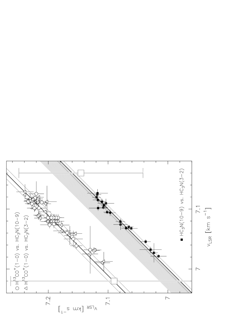
Figure 5: Correlations between the velocities of three different pairs of transitions, in the L 1512 area described in the text. Filled squares: HC₃N(10 – 9) vs. HC₃N(3 – 2); open circles: H¹³CO⁺(1 – 0) vs. HC₃N(10 – 9); open triangles: H¹³CO⁺(1 – 0) vs. HC₃N(3 – 2). For demonstration we assume here for the H¹³CO⁺(1 – 0) primary’s frequency the Woods et al. value, indicated on the left by the open square and its error bars, to be the correct one; the much more adequate Guélin et al. frequency is correspondingly depicted by the open square on the right. The dark diagonals represent the best linear fits of the correlations under the assumption that velocity offsets between transitions are constant over the whole field. Fainter diagonals show the rms deviations from these best linear fits. The shaded ribbon delineates the velocity uncertainty necessarily inherent in any H¹³CO⁺(1 – 0) interpretation that employs the correct rest frequency but does not take hyperfine splitting into account; points of high optical depth accumulate near the ribbon’s upper edge.

Our H¹³CO⁺(1 – 0) observations and their simultaneously measured HC₃N(10 – 9) counterparts likewise show a clear correlation with each other, as demonstrated by the open circles of Fig. 5. Here, we arbitrarily chose the Woods et al. (1981) frequency of 86754.329 MHz for the primary component of H¹³CO⁺(1 – 0). The corresponding H¹³CO⁺ correlation with HC₃N(3 – 2) (open triangles) is indistinguishably similar to that with (10 – 9) as far as the mean velocity difference is concerned, so that we coadded the two correlations to arrive at a H¹³CO⁺(1 – 0) – HC₃N difference of the signal-to-noise-squared weighted mean velocities of 0.1066 $\pm$ 0.0120 km s^-1 for 24 truly independent H¹³CO⁺(1 – 0) data points. This corresponds to 30.8 $\pm$ 3.5 kHz by which the Woods et al. frequency must be lowered in order to achieve velocity concordance between H¹³CO⁺ and HC₃N. We thus arrive at a frequency of 86754.2982 $\pm$ .0035 MHz for the primary line of the H¹³CO⁺(1 – 0) doublet, and of 86754.2589 $\pm$ .0069 MHz for the secondary. (The latter error is larger due to the uncertainty in the precise magnitude of the hyperfine split). The best value for single-component interpretations of the doublet would thus be 86754.2884 MHz, a mere 6 kHz or 0.02 km s^-1 away from the result of Guélin, Langer and Wilson(1982). Note that all errors given here are (very conservatively) rms deviations from the mean; for $\approx$20 independent data, the formal statistical error should be considerably smaller still. But even these rms values improve on published errors by factors of order 10, as shown by the large open squares in Fig. 5 which represent Woods et al.(1981) left, Guélin et al.(1982) right, both with their error bars.

The apparent drop near the left end of the H¹³CO⁺(1 – 0) – HC₃N correlation is not indicative of a realistic degree of true uncertainties but has an astronomical reason: these points all lie on the periphery of the cloud core where redshifted emission from the core mixes with the blueshifted one from surrounding gas. In these regions the ratio of blue to red contributions varies from species to species. For the mean and rms values these points are, however, not of concern.

Based on our improved (1 – 0) frequencies, on the (2 – 1) frequency from Bogey et al. (1981), and on the (3 – 2) frequency recently proposed by Gregersen & Evans (2001) we have redetermined the spectroscopic constants of H¹³CO⁺ which are presented in Table 4 together with their previous values from Bogey et al. (1981). Our unsplit line frequencies for the (2 – 1), (3 – 2) and (4 – 3) transitions, calculated with these new constants, are included in Table 3. Additional predictions are available in the CDMS (Müller et al. 2001). Their hyperfine pattern consists basically of two features separated by $\approx$ 20 kHz. With increasing transition frequency such splitting becomes very hard to resolve because of the increasing frequency width of the lines.

Table 4: Spectroscopic constants^a (MHz) of H¹³CO⁺ as determined from the present astronomical observations, compared with previous values^b.

parameter	valueb
$B$	43377	.3011(27)
	43377	.320(40)
$D$ $\times$ 10-3	78	.37(39)
	78	.3(75)
$C$(13C) $\times$ 10-3	18	.9(39)
$C$(H) $\times$ 10-3	–5	.55c
$d$ $\times$ 10-3	–25	.0c

^a Numbers in parentheses are one standard deviation in units of the least significant digit

^b In italics; Bogey et al. (1981)

^c Fixed to calculated value, see Table 1 and text

Both our (1 – 0) and (2 – 1) frequencies are at the lower end of the ranges given by Woods et al. (1981) resp. Bogey et al. (1981). Since the (2 – 1) laboratory frequency contributes only little to our spectroscopic constants (because of its large uncertainty), the very good agreement of our (3 – 2) prediction with the astronomical value from Gregersen & Evans (2001) comes as no surprise.

Simultaneous measurements of HC¹⁸O⁺(1 – 0) and H¹³CO⁺(1 – 0) finally led to a transition frequency of 85162.2231 $\pm$ 0.0048 MHz for the former, which itself has hyperfine splitting on the order of 8 kHz with a line strength ratio of 1:2. The primary’s value thus is some 2.7 kHz lower; see Table 2.

7 Can this hyperfine structure be of importance?

One might think that a line splitting of not more than the thermal width of very cold ($\approx$ 10 K) interstellar gas could hardly affect the interpretation of measured line profiles. We now want to give some examples to the contrary.

7.1 The case of L 1544

The first example for the potential usefulness of the doublet structure of H¹³CO⁺ concerns a recent publication by Caselli et al. (2002). These authors mapped a number of HCO⁺ and other isotopomers in the dense infalling core of L 1544 and presented high resolution line profiles from its central dust emission peak. In accordance with previous results (e.g. Tafalla et al., 1998) they found many optically thin lines to show double or highly asymmetric profiles toward the dust peak. With self-absorption being unlikely for very thin lines, they argued for two separate velocity components along the line of sight to the dust peak (here: “blue” and “red” for short) which they discussed in the framework of the Ciolek & Basu (2000) model of an almost edge-on disk that is radially contracting; the central region is thought to be depleted in CO-related species. The authors noted the H¹³CO⁺(1 – 0) profile to be remarkably different from the other five HCO⁺ isotopomer transitions which they presented for the dust peak. The former is much broader than the others, suggesting it to be optically thick, and its blue and red velocity components are separated by 0.36 km s^-1, in contrast to the $\approx$ 0.24 km s^-1 that hold for all the others.

We display their (1 – 0) profiles of HC¹⁸O⁺ and H¹³CO⁺ in Figs. 6a and b (dark histograms).

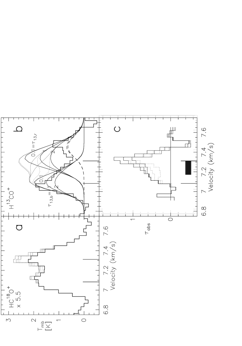
Figure 6: Observed L 1544 spectra (dark histograms) of a) HC¹⁸O⁺(1 – 0) multiplied by 5.5, and of b) H¹³CO⁺(1 – 0); after Caselli et al. (2002). Vertical bars mark the centers of the “blue” and “red” velocity components of HC¹⁸O⁺(1 – 0) and of numerous other transitions. Superimposed on b) are synthetic H¹³CO⁺(1 – 0) spectra as extrapolated from each of these two HC¹⁸O⁺(1 – 0) components alone (smooth dark lines) and from their combinations (light colors, see text); assumed H¹³CO⁺ optical depths are indicated. Dashed lines give the “red” component’s secondary contribution alone, without which the measured profile could not be fitted easily (see text). c) Optical depth of absorbing foreground material. The fat horizontal bar delimits the interval of bulk velocity of the absorbing gas. Light histograms in a) show HC¹⁸O⁺(1 – 0) profiles corrected for this presumed foreground absorption.

In the latter, a deep trough is seen that might stem from foreground absorption, while the dip in the former should rather reflect the separation of the two distinct velocity components mentioned, because this dip is seen in HC¹⁷O⁺ as well.

Assuming the two isotopomers’ excitation temperatures to be equal and, as also the abundance ratio, to be constant along the line of sight, we could calculate the H¹³CO⁺(1 – 0) doublet emission profile that should correspond to the HC¹⁸O⁺ spectrum, provided $\tau_{18}$ were known. Since the optical depths $\tau_{18}$ of both the blue and red velocity components of HC¹⁸O⁺ are a priori unknown, we choose a series of trial values for either and multiply them by an abundance ratio ¹³C:¹⁸O like, e.g., 7.3 to obtain $\tau_{13,b}$ and $\tau_{13,r}$.

With these we compute blue and red H¹³CO⁺(1 – 0) profiles like the dark smooth lines of Fig. 6b which, from top to bottom, correspond to H¹³CO⁺(1 – 0) optical depths of 0.1, 1 and 2 as indicated in the figure. These are total optical depths, i.e. the primary and secondary hyperfine component taken together. Three quarters of these values, or 5.5$\times\tau_{18}$, would be the optical depths of the primary hyperfine component. Combining the blue synthetic spectrum for optical depth 0.1 (because only low optical depths satisfy the observation) with the red one for $\tau_{13,r}$ either 0.1, 1 or 2 then gives the total synthetic H¹³CO⁺(1 – 0) profiles (the grey curves); full lines for the case that blue and red components are spatially separated in the beam, dotted lines for blue beyond (and thus partially absorbed by) red.

Correspondence between the published spectrum and the synthesised ones is quite close outside the absorbed central velocity interval. In particular, the high-velocity flank is very well described when hyperfine structure is taken account of. There is now no need for the H¹³CO⁺ lines being intrinsically broader than those of other species, or for particularly large optical thickness, or an exceptional increase in velocity separation between the red and the blue components. The cause is the red secondary hf component, depicted for itself as the dashed curves in Fig. 6b. This varies little with the particular choice of $\tau_{18,r}$ as optical depth effects would come into play here only at inappropriately large values of $\tau_{18,r}$. Any value that makes $\tau_{13,r}$ not much larger than 2 seems compatible with the data. On the other hand, $\tau_{13,{\bf b}}$ can hardly exceed unity; that component is likely optically thin.

We may imagine the H¹³CO⁺ absorption trough to be caused by a sheet of low-excitation gas placed in front of the emitting volume. Division of the observed by one of the calculated profiles then leads to that sheet’s optical depth as a function of velocity, at least if the sheet’s own emission is negligibly small. This velocity dependence becomes much clearer after the secondary’s contribution to absorption has been subtracted out. Fig. 6c shows $\tau_{abs}$ (the optical depth of the foreground primary alone). $5.5^{-1}$ of it should be the absorbing depth of foreground HC¹⁸O⁺(1 – 0) if the above assumptions continue to hold in the absorbing medium, too. Then, correction of the observed HC¹⁸O⁺(1 – 0) profile of Fig. 6a for this selfabsorption results in the grey step profiles. These in turn entail a slightly different set of synthetic H¹³CO⁺(1 – 0) profiles; changes are only minute, however.

Quite independently of the value we choose for $\tau_{18,r}$ and of the mode of combining blue and red in the beam, $\tau_{abs}$ seems composed of two distinct contributions, a very narrow one of width 0.12 km s^-1, i.e. the thermal width of 9 K gas, and a weaker, broader one. The narrow one is centered exactly on the velocity center of the red component of the total line profile, the broader one declines smoothly from there toward lower velocities, disappearing before reaching the blue component’s velocity center. (Note that with “velocity center” and “linewidth” we here mean that of the primary alone; both are identical with those of HC¹⁸O⁺ but for a 0.004 km s^-1 increase in the width). Since the absorbing linewidth must be at least thermal, the macroscopic gas velocities excluding thermal at which foreground absorption takes place are limited to the dark bar region in Fig. 6c, between approximately the assumed v_LSR of L 1544 (the mean between the blue and red line centers) and the red line center itself; nothing beyond on either side. The blue component seems to be without any absorbing cover of its own, in our direction.

The linewidth of $\approx$ 0.24 km s^-1 that both isotopomers show in their red emission component is considerably larger than the 0.12 km s^-1 of the contributor to absorption which is placed exactly at the velocity center of that red component, velocity-wise. The centrality of this position makes a velocity gradient a somewhat unlikely cause for the large width of 0.24 km s^-1; rather, it seems to speak for some kind of turbulent origin for this width.

7.2 Other examples

Takakuwa, Mikami and Saito (1998) have presented an interesting comparison between H¹³CO⁺ and CH₃OH emission from prestellar dense cores in TMC-1C. They argue convincingly that the two species trace different stages in the evolution of collapsing clumps since methanol is abundant at early stages while HCO⁺, being made from CO, accumulates only after CO has been amply produced. Consequently they expect somewhat different physical properties, on average, between the cores displaying predominantly CH₃OH and those with H¹³CO⁺ being prevalent. Instead, they observe no difference in size, linewidth or virial mass between the two groups in spite of their clear chemical differences. In particular, mean linewidths are found to be 0.33$\pm$0.11 km s^-1 for the ion versus 0.31$\pm$.09 for methanol.

These are narrow widths, hence the H¹³CO⁺ value should be discussed with caution. We have computed the reduction in true width to be expected when the hyperfine structure of H¹³CO⁺ is fully taken into account, binning our channels to their velocity resolution of 0.13 km s^-1. The result depends on optical depth. For very low values of $\tau_{13}$, the average width reduction is 0.055 km s^-1, marginally compatible with both chemical groups being of equal widths. For $\tau_{13}$ values of unity or above, the average width reduction would be 0.10 km s^-1 or roughly one third their value that was obtained without regard to hyperfine structure, and this would introduce a clear kinematical distinction between early and late clumps. Also, their virial masses would then have to be reduced correspondingly, halving the mean value to 1.2 $M_{\odot}$ for the H¹³CO⁺ clumps, just about equal to their mean LTE mass of 1.4 $M_{\odot}$. Since the damping of turbulence during core evolution poses interesting questions, high-resolution, high signal-to-noise observations of H¹³CO⁺ would seem very desirable.

Another topic where precise interpretation of H¹³CO⁺(1 – 0) linewidths might become useful concerns the determination of magnetic fields in dark clouds by comparing the widths of ions and neutrals as suggested by Houde et al. (2000). Results obtained from the lowest rotational transitions of H¹³CO⁺ and H¹³CN (Lai et al. 2003) indicate width differences in DR21(OH) to be on the order of the ion’s hf splitting, hence might be altered (and enhanced) when this splitting is taken into account.

A related effort by Greaves & Holland (1999) of comparing H¹³CO⁺(4 – 3) to ³⁴CS(7 – 6) velocities, instead of linewidths, seems inconclusive because their use of a rest frequency more uncertain than ours (Table 3) for the former species results in velocity errors larger than the velocity differences they measure at various positions. Indeed, their correlation between this difference and the alignment of grains as derived from continuum polarization all but vanishes once the new H¹³CO⁺ rest frequency is employed.

8 Observation of hyperfine structure in ¹³CO(1 – 0)

Having realised the analytical potential of the hyperfine splitting in H¹³CO⁺ we started to search for a similar situation in ¹³CO. The lowest rotational transition of this molecule had recently been calculated (see CDMS 2001, based on Klapper et al. 2000) and observed in the laboratory (Cazzoli et al. 2002a) to be splitting into two components, of frequency difference about 46 kHz (see Table 3), or also 0.13 km s^-1 in velocity space. The line strength ratio is 2:1 in favor of the higher frequency component. Since ¹³CO is a ubiquitous molecule in interstellar space it would be tempting to apply an analysis comparable to the preceeding one to the huge amount of available ¹³CO data. However, linewidths are usually large enough to drown any hyperfine effects; consequently, no such investigation seems to have been attempted to date.

The dark cloud L 1512 has, as mentioned, zones of exceptionally narrow lines in numerous species. Here, even ¹³CO widths can be as low as 0.35 km s^-1, sufficiently narrow to warrant attention to the hyperfine splitting if comparison with other lines is to be carried out. We therefore searched for hfs effects in the most dominant of these zones. We used the extensive IKP CO survey of this object (Falgarone et al. 1998) which covers a 300${}^{\prime\prime}\times 400^{\prime\prime}$ field in the relevant transitions. Nearly the whole IKP field emits strong (T_mb $\approx$ 6 K) ¹³CO(1 – 0) radiation of relatively smooth spatial structure. C¹⁸O, on the other hand, is more concentrated in a small number of clumps, the most prominent of which coincides with the H¹³CO⁺ clump discussed above. We chose a 100^′′$\times$100^′′ field centered on this clump to investigate hfs effects in ¹³CO. To improve the signal-to-noise ratio we coadded four nearest neighbors in the IKP data set for all of the following. For the purpose of this hfs study we make the simplest of possible assumptions, namely that excitation temperature and beam filling factor do not vary along each line of sight.

8.1 The line profiles

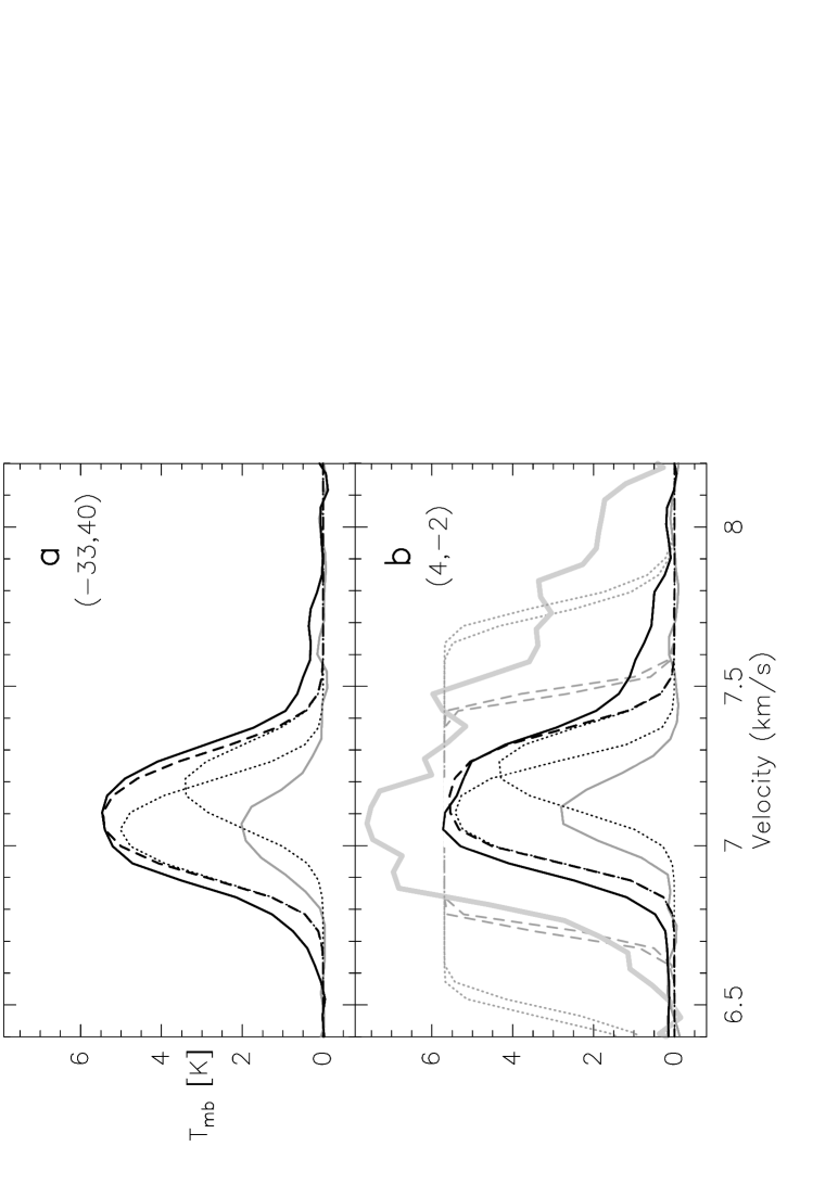
Figure 7: L 1512 spectra of ¹³CO(1 – 0) (full black curves) and of C¹⁸O(1 – 0) (full grey), observed at the offsets indicated (in arcsec). Dashed black curves show the ¹³CO doublet profiles that would be extrapolated from the C¹⁸O profiles as described in the text; black dotted lines mark the individual emissions from their two hyperfine components. Panel b) also displays the ¹²CO(1 – 0) emission (heavy light-grey); the flat-topped dashed grey curves give extrapolations (under simplifying assumptions) from hfs-corrected ¹³CO when a ¹²CO:¹³CO abundance ratio of 40 or 70 is applied. Wide grey-dotted profiles: Same when no hfs correction is taken into account.

Quite generally, the ¹³CO(1 – 0) and C¹⁸O(1 - 0) IKP spectra from any one position in this clump do not, at first sight, seem to have much in common. Assuming singlets for both lines, no reasonable abundance ratio would explain their large linewidth differences and relative v_LSR offsets. When hyperfine structure is properly taken into account, however, a close relationship becomes apparent. This is demonstrated by the typical line profiles shown in Fig. 7; a: from near the clump’s top edge, b: from close to its center. Assuming T_ex to be equal for both species in such a high density region, and positing a value for A, the ¹³CO to C¹⁸O abundance ratio, one could calculate the doublet profiles of ¹³CO(1 – 0) that would correspond exactly to the observed C¹⁸O profiles, if only $\tau_{18}$, the optical depths of the latter, were known. By varying $\tau_{18}$ and comparing the ¹³CO calculation to observation one obtains an estimate of the actual magnitude of $\tau_{18}$. Such resulting calculated ¹³CO(1 –0) profiles of maximal 18–13 correspondence are entered as the black dashed lines in Figs. 7a and b. Although these synthetic ¹³CO profiles are still marginally narrower than the observed ones, the correspondence is tempting and leaves little room for an all too different emission regime for the two lines.

That the consideration of hyperfine structure may render comparison of ¹³CO profiles with other isotopomers more fruitful is underlined in Fig. 7b where ¹²CO(1 – 0) is shown (fat light-grey) as well. Were one to take the intrinsic (individual hfs component) linewidth of the best-fit synthetic ¹³CO profile and its best-fit optical depth, and multiplied the latter by a ¹²CO:¹³CO abundance ratio factor of $\approx$ 40 or 70, one would obtain one of the grey dashed profiles as an expectation for ¹²CO(1 – 0), compatible on the low-velocity side with the actual observation. Were one to disregard hfs and take the full observed width of ¹³CO as indication of a high value of $\tau_{13}$ instead, much wider ¹²CO profiles like the dotted ones would result because of the correspondingly higher values of $\tau_{12}$.

Note that at the position near the clump’s edge (Fig. 7a), ¹³CO observation and construction are well centered on each other while in the clump’s more central region there is a clear shift between the two. One possible explanation could be absorption by “wing” material that is seen here in emission above 7.4 km s^-1 in both the ¹²CO and ¹³CO spectra. Such “wings” on ¹³CO, present at numerous positions in the core, are a major handicap for determining $\tau_{13}$, the total peak optical depth of ¹³CO, via hfs. Therefore, the following figures are meant to demonstrate trends and possibilities of analysis rather than to produce hard numbers. We have verified that the trends depend little on where wing cutoffs are placed.

8.2 The potential of hyperfine analysis of ¹³CO

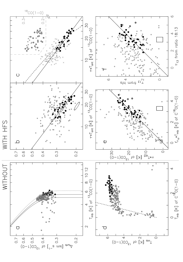
Figure 8: Properties of ¹³CO(1 – 0) and C¹⁸O(1 – 0) in the core field (black dots) and the full IKP field (grey dots) of L 1512. a-c) ¹³CO analysed for itself, d-f) in conjunction with C¹⁸O. Left column: results obtained without considering hyperfine splitting, right columns: taking hfs into account. Error sizes for the black dots are given in panels b, e and f by large open symbols. $\Delta v_{turb}$ is linewidth after substraction of a thermal component of 10 K. a) Smooth curves represent limits derived from the linewidth-optical depth relation. b) Decrease of linewidth with increasing optical depth (note that T_ant hardly varies over the core field). The straight line is the square root relation between the two quantities. c) Same as b) but with additional consideration of C¹⁸O data. d) Optically thin positions would have to fall along the dotted line if the ¹³CO:¹⁸CO abundance ratio were constant at 6.1 over the field. e) Close correspondence between ¹³CO and C¹⁸O emission in the core region becomes evident after C¹⁸O intensity is multiplied by the optical depth factor derived from analysing ¹³CO. f) Comparison of two independent methods of determining ¹³CO optical depth (hyperfine analysis vs. amplitude ratio). Note the underabundance of C¹⁸O outside the core region, evident in both e) and f).

Clearly the extra information contained in ¹³CO hyperfine structure provides insights into the physics of L 1512 that deepen those already published by Falgarone et al. (1998) and Heithausen et al. (1999). With $\tau_{13}$ known the physical quantity T_ex resp. T_ant can now be obtained from T_mb according to T_mb = $f_{bf}\cdot$T${}_{ant}\cdot$(1-$e^{-\tau})$. True linewidths of individual components of the doublet can be determined, sometimes giving values considerably smaller than what interpretation in terms of a single line might suggest. Such singlet interpretation is bound to also introduce errors in v_LSR, of up to some 0.04 km s^-1 depending on optical depth which influences the center of gravity of the doublet (cf. Fig. 5). Finally, the (hidden) correspondence between the seemingly uncorrelated ¹³CO and C¹⁸O lines puts comparisons between the two isotopomers on a much firmer basis.

We will not reanalyse the IKP data here but only sketch the usefulness of hfs analysis for the L 1512 core when its material becomes opaque in the ¹³CO (1 – 0) doublet. Non-hfs results of Falgarone et al. (1998) and Heithausen et al. (1999) are redrawn in Figs. 8a and 8d, distinction now being made between core positions (black dots) and the whole remaining IKP field (grey) excepting points of too weak a signal; hollow black points are to be excluded for good reason, e.g. superposition of two velocities. Since one-Gauss fits are poor approximations to overlapping doublet profiles, our Figs. 8a and 8d employ peak intensities and second velocity moments instead of the corresponding one-Gauss quantities. (Note that in Figs. 8a-c linewidth is shown as $\Delta v_{turb}$, i.e. after subtracting out a 10 K thermal contribution).

Immediately obvious in both figures is the apparent lack of any correlation for the black dots. This is because all over the core, T_ant(13) lies in the narrow range between 5.5 and 6.2 K (which corresponds to T_ex between 8.8 and 9.5 K), and $\tau_{13}$ exceeds 2, making T_mb more or less a surface quantity that is not meaningfully compared to a bulk property like linewidth. The inverse linewidth-peak intensity correlation extensively discussed by Falgarone et al.(1998) must not, therefore, be applied to opaque condensations like the core of L 1512. What then could take its place? The straightforward extension of T_mb into the regime of larger optical depths is $\tau\cdot$T_ant, a quantity accessible to observation via hfs analysis. Substituting this quantity for T_mb in Figs. 8a and 8d, and defining the ordinate $\Delta v_{turb}$ to now mean the intrinsic linewidth of the individual hfs components, clear correlations then appear as seen in Figs. 8b and 8e. In particular, since T_ant(13) has turned out to be very nearly constant over the core, a relation close to $\Delta v_{turb}\propto\tau_{13}^{-1/2}$ (the straight line in Fig. 8b) emerges. Also, the non-correlation of the T_mb values of the two isotopomers in Fig. 8d transforms into the linear correlation of Fig. 8e for the core points if a constant value for A (here: 6.1), hence for the unknown quantity $\tau_{18}$ (=$\tau_{13}\cdot{\it A}^{-1}$) is assumed. The factor f${}_{\tau_{13}}$ is $A^{-1}\cdot\tau_{13}\cdot(1-e^{-A^{-1}\cdot\tau_{13}})$. One thus finds T_ant of the two species to be within ten percent of each other all over the core region while outside, either $\tau_{18}$ or T_ant(18) seems to be wanting with respect to $\tau_{13}$ or T${}_{ant}(13)$. To the extent that in this high density region excitation temperatures at any given position are the same for the two species, this indicates that the assumption of a constant $\tau_{18}:\tau_{13}$ ratio is not valid for the IKP field at large; the abundance ratio there is different from the core’s.

How reliable are the $\tau_{13}$ values derived from hfs? Under the assumptions of equal T_ant values for both species (as expected for densities above 10⁴ cm^-3 where CO is thermalised) and of a constant abundance (hence $\tau$) ratio, $\tau_{13}$ can also be derived by the completely independent method of amplitude comparison between the two isotopomers. Results from these two unrelated methods are juxtaposed in Fig. 8f where the clustering of the core points along the equality line shows the effectiveness of the hfs method; at the same time the larger IKP field is seen to obviously be quite underabundant in C¹⁸O. This underabundance, which is likely caused by preferential UV destruction of C¹⁸O in the more transparent zones exterior to the core, must be the reason why the positions of low optical depths in Fig. 8d do not accumulate along a straight line like the dotted one (which represents an abundance ratio A of 6.1) as they should do if this ratio were constant across the IKP field.

8.3 Relation between linewidth and optical depth

Since for the core positions both methods of $\tau_{13}$ determination give similar values, they can be combined to reduce the noise in the final result. The improvement over Fig. 8b is shown in Fig. 8c, dark dots. With T_ant(13) practically constant all over the core, the $\Delta v-\tau$ relation (straight line) for this region then reads $\Delta v_{turb}=const\cdot\tau_{13}^{-1/2}$ with $const=0.46$ km s^-1. (Note that if $\tau\cdot T_{ant}$ were a power law function of total $\Delta v$ rather than of turbulent $\Delta v$ alone, the black points would accumulate along the dotted curve instead). Total ¹³CO column density $N_{{}^{13}CO}$ in LTE is $N_{{}^{13}CO}=2.56\times 10^{14}\cdot f_{bf}\cdot\tau_{13}\cdot\Delta v\cdot T_{ex}\cdot(1-e^{-T_{o}/T_{ex}})^{-1}$ cm^-2, with $\tau_{13}$ the sum of the peak optical depths of the two hfs components and $\Delta v$ the intrinsic width (including thermal) of either of them, measured in km s^-1. At T_ex around 9 K this means $N_{{}^{13}CO}$ around $5.2\times 10^{15}\cdot\tau_{13}\cdot\Delta v$ cm^-2 if $f_{bf}$ is equal to one. One thus arrives at the approximate further relation $\Delta v_{turb}=1.13\times 10^{15}\cdot N_{{}^{13}CO}^{-1}$ km s^-1. IKP data on C¹⁸O (inset) alone would be insufficient for determining such relations. (Note: for the inset the ordinate is linewidth of C¹⁸O without substraction of a thermal component).

For positions of weaker ¹³CO(1 – 0) lines, hfs analysis produces very uncertain values of $\tau_{13}$. One can make use of the near constancy of T_ex over the whole field by postulating a value of T_ex, here around 10 K, and then estimating $\tau_{13}$ from the measured value of T_mb(13). In Fig. 8c all points obtained in this way are entered as crosses as long as their $\tau\cdot$T_ant values are below 20 K. It thus emerges that the $\Delta v-\tau$ relation extends over much of the whole IKP field, provided the filling factor is unity everywhere.

With this relation both $\Delta v_{turb}$ and T_mb(13) are obtained as a function of $\tau_{13}$ once a value of T_ex is given. The ensuing $\Delta v_{turb}$-T_mb connections are shown in Fig. 8a by smooth curves depicting the cases T_ex(13) equal to 8.3 K, 8.8 K, and 9.5 K (dotted), respectively; the observed points fall closely between these curves in accordance with hfs analysis which has established this quite narrow T_ex regime over most of the field. The Falgarone et al. (1998) relation $\Delta v\propto T_{mb}^{-1}$ is now recognized as the limiting case of low optical depths.

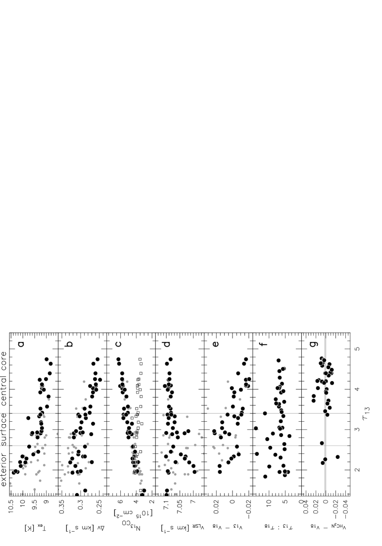
Figure 9: Physical properties of the extended core region of L 1512 (black dots) and of the IKP field at large (grey), as a function of ¹³CO optical depth. The two vertical lines refer to the black dots only. Panels a-d are derived from ¹³CO alone, e-f from ¹³CO and C¹⁸O combined. a) Excitation temperature, derived from T_ant by assuming beam filling factor unity. b) Total linewidth, i.e. including thermal, of a single hf component. c) Column density N${}_{{}^{13}CO}$, derived under the assumption of beam filling unity. Open squares show this quantity as determined without recourse to hyperfine analysis, dots the results obtained when employing hfs. d) v_LSR of ¹³CO(1 – 0), and e) relative motion between ¹³CO and C¹⁸O, both in km s^-1. f) Quotient of optical depths, indicative of the abundance ratio ¹³CO:C¹⁸O. g) v_LSR difference between HC₃N(3 – 2) and C¹⁸O(1 – 0) at selected positions in the core, in km s^-1; upper horizontal line is the mean value of the difference.

One simple picture to explain our power law relations would be of a quiescent, narrow-line core surrounded by a turbulent envelope, both of beam filling factor unity. Goodman et al. (1998) gave a thorough discussion of the transition from coherence to incoherence in dense cores. Also of particular relevance here are the recent observations by Kim & Hong (2002) who in numerous dark clouds found nearly no variation at all of the turbulent velocity dispersion with distance from center. Note that our results to the contrary, at least in the core of L 1512, would be largely washed out if we smeared out the IKP beam to their angular resolution of 50^′′. Our inside-out increase of $\Delta v_{turb}$ might be direct indication of the transition from a very quiescent nucleus to its turbulent envelope. Measurements in other objects would be desirable.

Finally, the slight width difference between the synthetic and the observed ¹³CO profiles of Figs. 7a and b may also find its natural explanation in the width-optical depth relation. It is in the outer, less opaque zones that the widest contributions to the line profiles are produced. These are also the zones of C¹⁸O underabundance. Hence relatively less widening in this isotopomer’s lines, thus also in the synthetic ¹³CO profiles derived from them, is to be expected.

8.4 Some physical properties of L 1512 as derived from hyperfine analysis

Fig. 9 summarises some physical trends, as recognised by hyperfine structure analysis, of the core plus its immediate ($\approx 25^{\prime\prime}$ wide) surroundings. The central core here is defined to comprise all positions with values of $\tau_{13}$ larger than 3.4, its immediate surface those between 2.6 and 3.4, and the exterior the values below. The top four panels result from ¹³CO hfs analysis alone, the lower ones from a combination with C¹⁸O.

Excitation temperatures (top panel) tend to decrease from outside in, as do the linewidths just discussed at some length. T_ex here is derived under the assumption of a constant beam filling factor equal to one. Since this might not hold in the surface region, the true value of T_ex there could be somewhat higher. Note that the excitation temperature of the main isotopomer, ¹²CO, is at 11.0 K all over the core’s surface (cp. Fig. 7b).

Column density (Fig. 9c; unity beam filling factor assumed) increases smoothly with $\tau_{13}$. In contrast, it would seem nearly constant (the open squares in the panel) if the standard method of deriving this quantity were followed. That method assumes equality of the excitation temperatures of ¹³CO and ¹²CO (the latter being measurable directly because of very large optical depths), and estimates $\tau_{13}$ by comparing the T_mb values of the two isotopomers. The assumption on T_ex is clearly not valid here, however, since ¹²CO is mainly emitted from the hotter surface, ¹³CO from the core. The difference makes for a factor up to 3 in optical depth. The corresponding difference in column density is somewhat lessened by the opposing difference in the values of linewidth (and in the T_ex(¹³CO)-dependent factor in $N_{{}^{13}CO}$), but even so, a profile interpretation employing hfs analysis arrives at column densities for the central core that are close to twice the “standard” values. This means similarly higher core mass. On the other hand, hfs analysis results in lower intrinsic linewidths, hence lower virial masses. Therefore, the net effect of taking account of the hyperfine splitting here is to make cores like L 1512 appear considerably more stable than when ignoring the splitting.

Fig. 9d: v_LSR of ¹³CO is at a well defined constant value for all positions but a few nearer the edge. However, close inspection shows the v_LSR difference (Fig. 9e) between the 13 and 18 isotopomers to vary from outside in, albeit very weakly; since the absolute v_LSR values are somewhat uncertain in the IKP data set, it is hard to say which species is more redshifted than the other. Since in the outer, more transparent regions both signals will stem to a larger extent from the same gas than further in, it is reasonable to suspect the central core (more visible in C¹⁸O than in ¹³CO) to be redshifted with respect to the surface. More precise measurements would be needed to quantify. Recall that at this level of variation, a sufficiently accurate determination of v_LSR(13) is only achievable by taking hyperfine structure into account.

The ratio of ¹³CO:C¹⁸O optical depths (Fig. 9f) directly reflects, in the central core, the abundance ratio of the two species. Higher values outside indicate C¹⁸O destruction beyond the region protected by large extinction.

Finally, Fig. 9g compares v_LSR of C¹⁸O(1 – 0) (as obtained from a small data set taken independently from IKP, of lower signal-to-noise ratio but more precise velocity determination) to that of the HC₃N(3 – 2) triplet mentioned above, at selected positions in or near the inner core. HC₃N optical depth in the core is found to be mostly on the order of 40 percent of that of ¹³CO, therefore in HC₃N and C¹⁸O one might see about the same regions with similar weight. In fact, no systematic velocity difference is recognisable at all between these two species except that their mean values differ by .0014 km s^-1 (the upper horizontal line) if the most precise measured C¹⁸O frequency (Cazzoli et al. 2003) is employed. This difference is not larger than the published uncertainties of either line and thus lends support to the accuracy of the H¹³CO⁺(1 – 0) frequency that was derived in section 6 via HC₃N.

9 Conclusions

We wanted to show in this paper that the ¹³C nucleus’ magnetic moment can provide a useful additional tool for analysing radiation from both the H¹³CO⁺ and the ¹³CO molecules. These species have not previously been investigated with consideration of this important detail. This is because the separation of their hyperfine components, 0.13 km s^-1 for both species, is as narrow as the thermal width of cold interstellar gas and therefore a rather quiescent cold astronomical target, high spectral resolution, and good signal-to-noise ratios are all required to observe the splitting. When these conditions are fulfilled, however, narrowness of separation is hardly a handicap: while partial overlap of the components does of course degrade information near the profile’s center, the noise in the totality of the line is also less than if the components were distinctly apart. One should also note that line strength ratios 3:1 or 2:1, as in the present cases, are next to ideal for retrieving astronomical quantities like optical depth. Ratios much closer to one would not allow clear determination of depth by comparison of amplitudes of the hyperfine components, much larger ones on the other hand would carry the risk of correlating gas regimes that might in reality be quite distinct, one of high optical depth, the other transparent.

For narrow-line regions, the determination of velocities profits most directly from knowing the hyperfine structure underlying a profile. Therefore we were able to present H¹³CO⁺ rotational transition frequencies of considerably improved precision by comparing to other, well-defined lines in L 1512, as well as to verify astronomically the ¹³CO(1 – 0) doublet frequencies first predicted by theory. This precision in turn allows studies of the internal motions of very quiescent clouds that may be extremely subsonic but, as was shown above for the case of L 1512, may nevertheless indicate the onset of collapse toward the center of a potentially star-forming core.

The inadequacy of interpreting a close-doublet profile by singlet analysis becomes very evident in the derivation of linewidths. Here, neglect of hyperfine structure in the profile can easily entail considerable overestimates which in turn lead to erroneous values of column density and of virial mass (the latter being proportional to the square of intrinsic linewidth). This effect is compounded by the frequently necessary neglect of line broadening caused by nonzero optical depth. In the case of the two ¹³C-containing species discussed here, the direct handle on optical depth that is provided by the nuclear magnetic moment may permit a more reliable determination of the intrinsic linewidth and its derivatives. For this reason, we were able to establish a width-depth or width-column density relation for the core of L 1512 that may eventually make the transition from a completely quiescent central core to a turbulent envelope accessible to observations. This more direct method of obtaining optical depths, rather than by the standard method for ¹³CO, allowed us to recognise the L 1512 core as considerably more bound than suspected since core mass has to be revised upwards and virial mass downwards upon considering line multiplicity correctly. Likewise we tried to argue that measurements in the dark core of L 1544 which seem to set H¹³CO⁺ quite apart from numerous other molecular species may in reality fall nicely in line when hyperfine splitting is properly considered.

A reestimate of H¹³CO⁺ linewidths also suggests that chemical evolution of collapsing cores over time should indeed be observable through the comparison of these linewidths with those of other molecules. Further, recent attempts to derive magnetic field strengths in molecular clouds by comparing ion linewidths with those of neutrals (H¹³CO⁺ vs. H¹³CN) should profit from taking the doublet nature of the ion into consideration. For all these reasons it is hoped that the hyperfine structure in the profiles of the species discussed in this paper will motivate further high-resolution studies of cold dark clouds.

- (1) Bogey M., Demuynck C., Destombes, J. L. 1981, Mol. Phys., 43, 1043
- (2) Botschwina P., Horn M., Flügge J., Seeger S. 1993, Faraday Trans., 89, 2219
- (3) Caselli P., Myers P. C., Thaddeus P. 1995, ApJ, 455, L77
- (4) Caselli P., Walmsley C. M., Zucconi A., et al. 2002, ApJ, 565, 331
- (5) Cazzoli G., Puzzarini C., Lapinov A. V. 2003, ApJ, 592, L95
- (6) Cazzoli G., Dore L., Cludi L. et al. 2002a, J. Mol. Spectrosc., 215, 160
- (7) Cazzoli G., Dore L., Puzzarini C., Beninati S. 2002b, Phys. Chem. Chem. Phys., 4, 3575
- (8) CDMS (2001): Cologne Database for Molecular Spectroscopy: Müller H. S. P., Thorwirth S., Roth D. A., Winnewisser G. 2001, Astron. Astrophys. 370, L49 (http://www.ph1.uni-koeln.de/vorhersagen/index.html)
- (9) Ciolek G. E., Basu S. 2000, ApJ, 529, 925
- (10) Coxon J. A., Hajigeorgiou P. G. 1992 Can. J. Phys., 70, 40
- (11) Creswell R. A., Winnewisser G., Gerry M. C. L. 1977 J. Mol. Spectrosc., 65, 420
- (12) Dore, L., Puzzarini, C., Cazzoli, G. 2001, Can. J. Phys., 79, 359
- (13) Ebenstein, W. L., Muenter, J. S. 1984, J. Chem. Phys., 80, 3989
- (14) Falgarone E., Panis J. F., Heithausen A., Perault M., Stutzki J., Puget J. L., Bensch F. 1998, Astron. Astrophys. 331, 669
- (15) Fiebig D. 1990, PhD Thesis Universität Bonn
- (16) Garvey, R. M., De Lucia, F. C. 1974, J. Mol. Spectrosc., 50, 38
- (17) Goodman A. A., Barranco J. A., Wilner D. J., Heyer M. H. 1998, ApJ, 504, 223
- (18) Greaves J. S., Holland W. S. 1999, MNRAS, 302, L45
- (19) Gregersen E. M., Evans II N. J. 2001, ApJ, 553, 1042
- (20) Guélin M., Langer W. D., Wilson R. W. 1982, Astron. Astrophys. 107, 107
- (21) Heithausen A., Stutzki J., Bensch F., Falgarone E., Panis J. F. 1999, Rev. Mod. Astron., 12, 201
- (22) Helgaker T., Jensen H. J. Aa., Jørgensen P., et al. Dalton release 1.0 (1997), an electronic structure program
- (23) Hirota T., Ikeda M., Yamamoto S. 2003, ApJ, 594, 859
- (24) Houde M., Bastien P., Peng P., Phillips T. G., Yoshida H. 2000, ApJ, 536, 857
- (25) Irvine W. M., Goldsmith P. F., Hjalmarson A. 1987, in Interstellar Processes, eds. D. Hollenbach and H. A. Thronson (Dordrecht: D. Reidel), 561
- (26) Jensen H. J. Aa., Jørgensen P., Agren H., Olsen J. 1988a J. Chem. Phys., 88, 3834
- (27) Jensen H. J. Aa., Jørgensen P., Agren H., Olsen J. 1988b J. Chem. Phys., 89, 5354
- (28) Kim H. G., Hong S. S. 2002, ApJ, 567, 376
- (29) Klapper, G., Lewen, F., Gendriesch, R., Belov, S. P., Winnewisser, G. 2000, J. Mol. Spectrosc., 201, 124
- (30) Lai S.-P., Velusamy T., Langer W. D. 2003, preprint
- (31) Klapper, G., Lewen, F., Gendriesch, R., Belov, S. P., Winnewisser, G. 2001, Z. Naturforsch., 56a, 329
- (32) Maki A. G., Mellau G. Ch., Klee S., Winnewisser M., Quapp W. 2000, J. Mol. Spectrosc., 202, 67
- (33) Muders D. 1995, PhD Thesis Universität Bonn
- (34) Myers P. C., Benson P. J. 1983, ApJ, 266, 309
- (35) Pickett H. M., Poynter R. L., Cohen E. A., Delitsky M. L., Pearson J. C., Müller H. S. P. 1998, J. Quant. Spectrosc. Radiat. Transfer, 60, 883
- (36) Snyder L. E., Hollis J. M., Lovas F. J., Ulich B. L. 1976, ApJ, 209, 67
- (37) Tafalla M., Mardones D., Myers, P. C., Caselli P., Bachiller R., Benson P. J. 1998, ApJ, 504, 900
- (38) Takakuwa S., Mikami H., Saito M. 1998, ApJ, 501, 723
- (39) Thorwirth S., Müller H. S. P., Winnewisser G. 2000, J. Mol. Spectrosc., 204, 133
- (40) Winnewisser M., Winnewisser B. P., Winnewisser G. 1985, in Molecular Astrophysics, Series C, eds. G. H. F. Diercksen, W. F. Huebner, and P. W. Langhoff (Dordrecht: D. Reidel), 375
- (41) Woods R. C., Saykally R. J., Anderson T. G., Dixon T. A., Szanto P. G. 1981, J. Chem. Phys., 75, 4256