$p$-mode frequencies in solar-like stars:

As a part of an on-going program to explore the signature of $p$-modes in solar-like stars by means of high-resolution absorption line spectroscopy, we have studied four stars ($\alpha$ CMi, $\eta$ Cas A, $\zeta$ Her A and $\beta$ Vir). We present here new results from two-site observations of Procyon A acquired over twelve nights in 1999. Oscillation frequencies for $l$=1 and 0 (or 2) $p$-modes are detected in the power spectra of these Doppler shift measurements. A frequency analysis points out the difficulties of the classical asymptotic theory in representing the $p$-mode spectrum of Procyon A.

1 Introduction

Precise measurements of the frequencies and amplitudes of the solar five-minute oscillations have led to detailed inferences about the solar internal structure (cf. review paper by Christensen-Dalsgaard 2002). Because of the wealth of knowledge obtained from helioseismology there is a strong impetus to use the pulsation analysis techniques to probe the interiors of solar-like stars. From the ground, the application of seismic techniques to these stars is difficult because of extremely small variations in intensity and velocity associated with $p$-modes and the need to have an adequate temporal coverage to resolve the modes. To detect such small amplitudes, photometric methods (Gilliland et al. 1993) suffer from scintillation noise unless conducted from space, e.g. MOST (Walker et al. 2003; Matthews et al. 2000) or the future COROT (Baglin 2003) and Eddington (Roxburgh & Favata 2003) missions. Recent developments in high-precision spectrometric techniques and, in particular, Doppler spectroscopy have led to the detection of $p$-mode frequencies in individual solar-like stars (e.g., Martic et al. 1999; Bedding et al. 2001; Martic et al. 2001b; Bouchy & Carrier 2002; Frandsen et al. 2002; Kjeldsen et al. 2003; Carrier & Bourban 2003). A recent review of these and other measurements has been given by Bedding & Kjeldsen (2003).

One of the most interesting target for solar-like seismology is Procyon A ($\alpha$ CMi, HR 2943, HD61421), a F5 IV star with $m_{\rm v}$=0.363 at a distance of only 3.53 pc. Its fundamental stellar parameters are now well determined. Procyon A is in a 40-year period visual binary system, sharing the systemic velocity with a white dwarf. Procyon’s astrometric orbit was recently updated by Girard et al. (2000). With a parallax, $\Pi=283.2\pm 1.5$ mas, they estimated a mass of $1.470\pm 0.045M_{\odot}$, which agrees well with previous excellent predictions from stellar interior models (Guenther & Demarque, 1993). In addition, Mozurkewich et al. (1991), using optical interferometry, measured a stellar angular diameter $\theta$ = 5.51$\pm 0.5$ mas. Adopting the very precisely measured parallax by Hipparcos, $\Pi=285.93\pm\,0.88$ mas, Prieto et al. (2002) derived a slightly lower mass of 1.42 $\pm\,0.06\rm\thinspace M_{\odot}$, a radius R/$\rm\thinspace R_{\odot}=2.071\,\pm\,0.02$ and a gravity log $g=3.96\,\pm 0.02$ (in cgs units).

An exploratory single-site Doppler observation of Procyon A by Martic et al. (1999), hereafter Paper I, revealed the presence of several frequencies that fell in a comb-like pattern with roughly equal spacing of $55\,\mu$Hz in the region of excess power around 1 mHz in the power spectrum. Because of the large daytime gaps in these single-site measurements, it was not possible to identify these frequencies unambiguously. Note however that the set of frequencies reported in Paper I were determined very close ($\leq 2\,\mu$Hz) to the model frequencies published independently by Chaboyer et al. (1999).

Following the findings of these exploratory studies we have carried out a two-site campaign of Procyon A to identify as many $p$-modes as possible without alias ambiguities. In section 1, we describe the context of the observing runs, in section 3 we present the periodograms of the time sequences from coordinated two-site measurements. In sections 4 and 5, we outline the different techniques we used to search for the $p$-modes in the power spectra. In the last sections, we present the principal mode characteristics (large and small separations, amplitudes) and compare the results with the existing models.

2 Observations and Data reduction

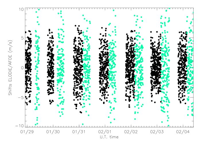
Figure 1: Doppler shift measurements over seven nights from two-sites observations of Procyon A (black dots: ELODIE data, green dots: AFOE data).

The observations were carried out with the ELODIE spectrograph mounted on the 1.93m OHP telescope, France and the Advanced Fibre-Optic Echelle (AFOE) spectrometer located at the 1.5m (60″) Tillinghast telescope of the Whipple Observatory, Arizona, USA. The ELODIE and AFOE are fiber-fed cross-dispersed echelle spectrographs (Baranne et al. 1996; Brown et al. 1994) that were optimized for precise and stable Doppler measurements. Both systems use double-fiber scramblers.

As configured for these coordinated measurements, AFOE covered 160 nm of spectrum lying between 393 and 665 nm (23 echelle orders) at a resolution of roughly $R\sim 32000$. The wavelength reference used for these observations was a ThAr emission-line spectrum brought into the spectrograph by a second optical fiber. The reduction steps for AFOE data are explained in Brown et al. (1997). A total number of 1127 extracted spectra, with sampling rate of about 140 s, has been used for this Doppler velocity time sequence analysis.

The ELODIE data were obtained as a continuous series of raw CCD (Tk 1024) frames with a sampling rate of about 100 s. We built an asteroseismic mode to automatically acquire long uninterrupted sequences of simultaneous stellar and reference (Fabry-Perot) exposures. The advantage of using the closely-spaced channelled spectrum from a fixed (ZERODUR) Fabry-Perot interferometer is that it gives the best possible reference even for very short exposure times (30 s for Procyon) and allows us to monitor with a high precision the spectrograph instabilities. In our configuration, the reduction process produces for each CCD frame a set of stellar and Fabry-Perot spectra, at a resolution of $R\sim 42000$, interleaved into 67 echelle orders, each covering 5.25 nm or in total a wavelength domain from 390.6 to 681.1 nm.

The radial velocity computation algorithm is based on the method proposed by Connes (1985) for the computation of the very small residual shifts with an absolute accelerometer. Our algorithm was first tested on $\psi$ UMa, HR4335 (see Connes et al. 1996) and optimized with a spline interpolation for the iterative Doppler shift calculation to take account of the larger shifts induced by earth motion and instrument drifts during the night (cf. Paper I).

The formalism of the Connes’ algorithm was summarized in Bouchy et al. (2001). It was recently used as the ”optimum weight procedure” by Bouchy & Carrier (2002) for the detection of the oscillations of $\alpha$ Cen and by Frandsen et al. (2002) for the giant star $\xi$ Hya. We should however note that the use of this method, for close echelle orders, is very sensitive to the star flux variation in the course of the night that induces an intensity-velocity correlation and in consequence a larger amplitude of the oscillation signal.

ELODIE (1999)				AFOE (1999)
Date	Nbr	T(hr)	$\sigma$(m s-1)	Date	Nbr	T(hr)	$\sigma$(m s-1)
01/27	232	5.56	5.64
01/28	214	5.51	2.76	01/29	92	3.84	5.21
01/29	233	5.57	2.70	01/30	155	6.15	4.00
01/30	282	8.30	3.18	01/31	171	6.79	4.21
01/31	287	8.44	2.71	02/01	166	6.59	3.90
02/01	354	8.45	2.70	02/02	194	7.78	3.84
02/02	389	9.28	2.40	02/03	196	7.79	4.49
02/03	266	7.82	2.75	02/04	153	6.08	4.02
02/05	336	7.93	3.43
02/06	280	8.08	3.00
02/07	269	8.01	2.87
02/09	101	3.00	3.08

Table 1: Observation log (UT)

Figure 2: Power spectrum of Procyon A from Doppler shift measurements over 15 hours, with ELODIE and AFOE.

ELODIE 1999

AFOE 1999

ELODIE/AFOE 1999

Simulations (ELODIE/AFOE)

Figure 3: Top panels: Power spectra of the ELODIE and AFOE Doppler shift measurements (7 nights) of Procyon. Bottom left panel: Power spectrum of the combined data sets. Bottom right panel: Simulated spectrum computed with noise and with the same observation times as the combined sequence ELODIE/AFOE.

Due to variable weather conditions and lower mean S/N than in our 1998 observations, we de-correlate the Doppler velocity from residual flux variations in and between the orders, used for the calculation of the final weighted mean Doppler signal.

A journal of Procyon A observations in 1999 is given in Table 1. The table lists the length of the individual runs in hours, the number of selected exposures and the rms scatter of the time series. To illustrate the precision of each data-set, we show in Fig. 1 the resulting Doppler signal from both sites.

3 Power spectra analysis

The power spectrum of the weighted mean Doppler shift measurements for one of the best nights (high S/N, low rms residual) of Procyon observations is presented in Fig. 2.

Inspection of the other single-night spectra confirms the presence of an excess power and several common peaks that modulate the envelope between 0.3 mHz and 1.7 mHz. Comparison of individual power spectra allows us to search for the repetitive occurrence of peaks, free from aliasing, from one night to an another, but the frequency resolution is too low to distinguish the mode fine structure. We find in a few cases large peaks which highly exceed the S/N in the region of the hump of power. This characteristic could be explained as ’large excitations’ from the studies of the solar p-mode spectrum (Elsworth et al. 1995). In the solar case, the lifetime of the strongest modes are only of the order of a few days and their evolution can be followed on a short time scale when their frequencies are visibly separated and free from mutual interferences. In our observations the occasionally large excitations stay visible in the power spectrum from three or four successive nights but more or less important interferences with noise have also to be considered. In general, the relative amplitudes of the frequencies vary from night to night, with the result that a given frequency may dominate the amplitude spectrum in some data segments and be entirely undetectable in the others. To address these issues, we performed many frequency analyses of the entire data set, numerous subsets of the data and simulated time series having the same sampling function as the observations.

In Fig. 3 (upper panels), we show the power spectra from ELODIE and AFOE one-site measurements of Procyon A over seven consecutive nights. Note that the observing run with the ELODIE/OHP spectrograph was longer, twelve nights (see periodogram in Martic et al. 2001b). The power spectra were calculated using the Lomb-Scargle (LS) modified algorithm (Lomb 1976; Scargle 1982) with statistical weights. The mean white noise level ($\sigma_{\rm hf\_ps}$), the rms scatter ($\sigma_{\rm ob}$), the frequency resolution and computation bin are indicated for each data set. The noise level is higher in the AFOE data, which makes less evident the excess of power in the low-frequency part of the spectra.

The time series from the two sites were merged by first subtracting a second order polynomial fit and the clipping data over $2\,\sigma$ for each night. This process yields similar rms scatter of data from one night to another and allows us to compute the power spectrum of combined time series without using weights (see bottom left panel of Fig. 3). To verify that the amplitude of the excess signal was not severely reduced by removing outlying points over $2\,\sigma$, we calculated also the power spectrum using statistical weights (1/$\sigma^{2}$) of the time sequence after $4\,\sigma$ clipping. By comparing these two power spectra, we note that the frequencies of the major peaks remain unchanged but with more power in the sidelobes of the weighted spectrum. For these data the application of the weights has not produced an important reduction in noise but rather degraded the window function.

One can see in Fig. 3 that the overall shape of the excess power around 1 mHz is not symmetric and does not have the typical bell-like envelope of the solar oscillations. This can be explained by the effects of gaps/noise and amplitude modulation that are intrinsic to the star (beating between pairs of modes that are closely spaced in frequency and finite lifetime of each oscillating mode). The effects of noise interference and the window function are visible in the power spectrum (see right lower panel of Fig. 3) of the simulated time series with an artificial oscillating signal and the rms almost equal to that of the observed data sets.

We performed several simulations in the presence of noise with the oscillation signal based on frequencies identified in section 5. The amplitude distribution of the generated signals was produced as in Barban et al. (1999) but with mode ($l,m$) ratios computed for updated Procyon parameters and with the maximum mode amplitude of about 35 cm/s near the peak of the excess power.

In the periodogram of the joint ELODIE and AFOE observations several isolated peaks are present between 0.3 mHz and 1.4 mHz, due to a much better window function (see the amplitude of the sidelobes in the inset of Fig. 3). These frequencies were used as starting ones for the comb power analysis and asymptotic fit calculations (cf. next section).

4 Echelle diagrams

In the solar case, the asymptotic theory (see e.g., Tassoul 1980) provides quite good results for the acoustic modes with high radial order $n$ and low degree $l$. The asymptotic relation is expected to hold for the solar-like $p$-mode oscillations in other stars and gives mode frequencies as

$$\nu({nl})=\Delta\nu(n+\frac{1}{2}l+\frac{1}{4}+\alpha)+\epsilon_{nl}$$ (1)

where $\Delta\nu$ is the inverse of twice the sound travel time between the centre and the surface, $\alpha$ is dependent on the reflective properties of the surface and $\epsilon_{nl}$ is a small correction term sensitive to the central structure of the star.

In the vicinity of some radial order $n_{0}$ one can parametrize the expected mode frequencies as

$$\nu(n_{\mathrm{p}},l)\simeq\nu_{0}+\Delta\nu_{0}(n_{\mathrm{p}}+\frac{1}{2}l)-l(l+1)D_{\rm 0}$$ (2)

where $n_{\mathrm{p}}=n-n_{0}$, $\nu_{0}$ is the frequency with $n=n_{0}$ and $l=0$, $\Delta\nu_{0}$ represents the so-called mean large frequency separation between $p$-modes of same degree and adjacent $n$. $D_{\rm 0}$ is related to the so-called small frequency separation $\delta\nu_{l,l+2}$ where $\delta\nu_{l,l+2}=\nu(n,l)-\nu(n-1,l+2)\simeq(4l+6)D_{\rm 0}$.

The third separation $\delta\nu_{0,1}$, which represents the amount by which $l$=1 modes are offset from the midpoint between the $l$=0 modes on either side (see e.g., Bedding & Kjeldsen 2003) can be defined as $\delta\nu_{0,1}=\nu(n,0)-\frac{1}{2}(\nu(n,1)+\nu(n-1,1))$. If the asymptotic relation holds exactly, $D_{\rm 0}=\frac{1}{6}\delta\nu_{02}=\frac{1}{10}\delta\nu_{13}=\frac{1}{2}\delta\nu_{01}$.

To the first order, a star pulsating with a number of consecutive radial modes of a given $l$ has a comb-like eigenspectrum with a spacing $\Delta\nu_{0}$ and if both even and odd $l$ modes are present, with spacing $\Delta\nu_{0}/2$. To estimate $\Delta\nu_{0}$ in the region of excess power of the Procyon frequency spectrum we used the comb response method.

In previous analysis of the single-site data (Martic et al. 2001a) we applied the comb analysis to the CLEAN-ed power spectra because of important aliases at spacings $\pm\,11.57\,\mu$Hz from the largest peaks. To improve the accuracy of these results and to see whether we can use the comb response (CR) to distinguish the even from odd $l$ mode frequencies, we rewrite the function (cf. Eq. 2 in Kjeldsen et al. 1995) as

Figure 4: Comparison between modified comb responses computed for two central frequencies of the power spectrum of Procyon data (see description in text).

$$C(\nu_{\mathrm{0}},\Delta\nu_{\mathrm{0}})=\prod_{i=0}^{4}\left[\,S(\nu_{\mathrm{0}}+i\frac{\Delta\nu_{\mathrm{0}}}{2}+\delta)\,S(\nu_{\mathrm{0}}-i\frac{\Delta\nu_{\mathrm{0}}}{2}+\delta)\right]^{\alpha_{i}}$$ (3)

where $\delta=\pm(i\bmod 2)D_{0}$ according to mode degree $l=0$ or $l=1$ at the central frequency $\nu_{0}$ and $\alpha_{i}=1$ for $i=1$ or 2, $\alpha_{i}=0.5$ for $i=3$ or 4.

Figure 5: Top panel: The first-order spacings over several frequency ranges, as determined from comb analysis. Bottom panel: Echelle diagram of the selected frequencies with the best comb responses ($l=0,1$ indicated respectively by diamonds and triangles).

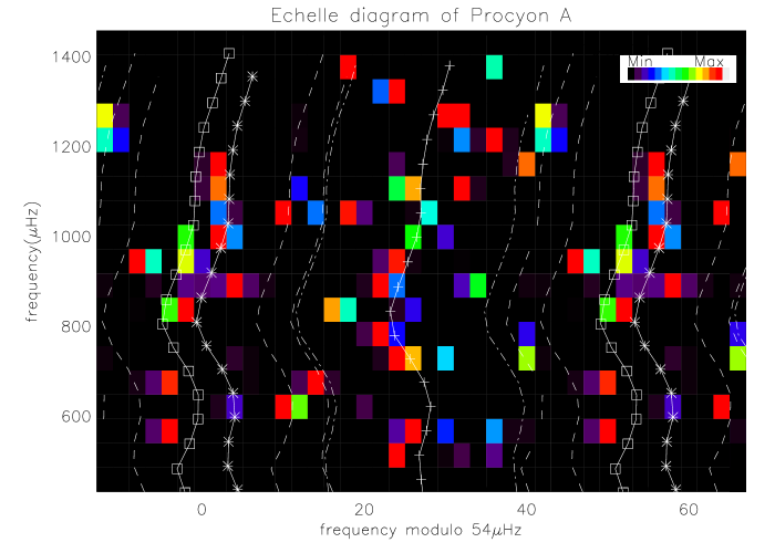
Figure 6: Example of an echelle diagram from Procyon amplitude spectrum of the joint ELODIE and AFOE radial velocity measurements, computed for the modulo mean $\Delta\nu_{\rm 0}$= 54 $\mu$Hz. The frequencies from the standard model (see Chaboyer et al. 1999) are indicated by asterisks, plus signs and squares respectively for $l=0,1,2$, dashed lines are at $l=0,1,2\pm\,11.6\mu$Hz). The inset shows the colour coding applied to the values in each succesive folding frequency range.

The modified comb responses (Eq. 3) were then calculated at the frequencies of the highest peaks in the power spectrum. For each central frequency $\nu_{0c}$, alternatively considered as $l=0$ and $l=1$, we have searched for the maximum CR for $10\,\leq\Delta\nu_{0}\leq 80\,\mu$Hz and $0.3\,\leq D_{\rm 0}\leq 2$.

In Fig. 4 we show examples of the modified comb response computed for two $\nu_{0c}$ frequencies at 753 $\mu$Hz and 776 $\mu$Hz. The responses are scaled to the maximum peak obtained at $53.5\,\mu$Hz when $\nu_{0c}$= 753 $\mu$Hz was assumed to be $l=0$.

From the initial set of the highest peaks corresponding to the modes, but also to the aliases, the comb analysis gives the reduced set of $\nu_{0c}$ frequencies and corresponding $\Delta\nu_{0c}$ for which the maximum CR is obtained. The upper panel of Fig. 5 shows the variation of the first-order spacing over several different frequency ranges, as determined from comb analysis. The arithmetic mean of these spacings is $54\,\mu$Hz, a value for a large separation in good agreement with the theoretical predictions from models (Chaboyer et al. 1999; Di Mauro & Christensen-Dalsgaard 2001; Provost et al. 2002). In addition, this exploration allowed us, from the comparison of the relative power of the best responses, to separate temporarily the modes by degree. In Fig. 5 (lower panel), we show these frequencies in the echelle diagram (cf. Grec et al. 1983) for the modulo mean $\Delta\nu_{\rm 0}$= 54 $\mu$Hz.

In a second step we calculate the echelle diagram so as to preserve the amplitude information. It can be constructed either from the power or CLEAN-ed spectra by adding (within cells of the order of the frequency bin) the values modulo large splitting, over threshold determined by the mean noise level of a time sequence. This means that any points lower than the noise level are set at this level. The echelle diagrams constructed in this way are used to compare the overall distribution of the power for different possible average splittings. In general, the ridge like structure appears for the mean $\Delta\nu_{\rm 0}$ determined from previous comb-like analyses. This method was first tested on solar data obtained with the same instrument during a daytime run. The echelle diagram of the single-site ELODIE observations were shown in Martic et al. (2001b) and discussed in Provost et al. (2002).

We should point out that the distribution of the power in these kinds of echelle representations depends greatly on the starting folding frequency $\nu_{0}$ and the threshold level, especially when mode amplitudes are decreased by destructive interference in some frequency ranges. In Fig. 6 we show an example of such an echelle diagram based on the ELODIE and AFOE joint observations. To increase the visibility of the modes in this image we modified the power spectrum by a simple normalization to the highest peak in each successive folding frequency range. The maximum power is concentrated in the ridge that is identified as $l=1$ and which shows the offset from $0.5\Delta\nu_{0}$ between the $l=0$ modes. The departure from a linear asymptotic relation is evident. It explains why, for the stars like Procyon, classical methods used for mode diagnostics are not easily applicable (cf. Bedding et al. 2001).

5 Mode identification

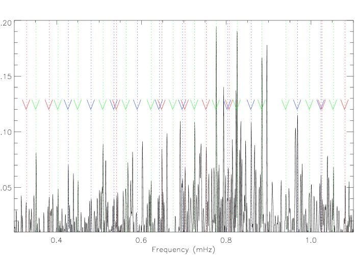
Figure 7: Identification of the $p$-modes in the region of the excess power of Procyon A. Dashed lines in blue, red and green correspond respectively to modes $l=2,0,1$.

The best values, based on our modified comb analysis, for $\nu_{0c}$, $\Delta\nu_{0c}$ and $D_{0c}$, were then used to reconstruct the parameterized frequencies in separate frequency regions ($\nu_{0c}\pm\,2\Delta\nu_{0c}$). These ’model’ frequencies have a significant departure from the asymptotic relation for one set of mean fit parameters. From this step, we have proceeded in an iterative manner to identify the modes.

The observed high amplitude frequencies were classified by degree comparing to the model ones and used to obtain new fit parameters by performing multidimensional minimization of Eq. 2. This method was used because we first selected the peaks with the strongest amplitudes, which means that successive $n_{\rm p}$, or l pairs of modes are not always present. We calculated the fit for various combinations of modes with different degree, using the downhill simplex method (Nelder & Mead 1965). A certain number of high amplitude frequencies were then shifted by $\pm\,11.57\,\mu$Hz and included in the selection of the modes, which improved the convergence (small max error). In Fig. 7, we show the selection of frequencies in the region of excess power at $4\,\sigma$ above the mean white noise, for which we obtained the best fit. The values for $\Delta\nu_{0}$ and $D_{0}$ from the fit are :

$\Delta\nu_{0}=53.6\,\mu$Hz

$D_{0}=0.85\,\mu$Hz, $\delta\nu_{02}\approx 6D_{0}=5.1\,\mu$Hz

Given the complexity of this spectrum, the noise background, the short mode lifetimes (cf. Brown et al. 1991) and the possibility of cross-talk between a real frequency and an alias etc., we checked the presence of this set of frequencies in other independent subsets of the data. We calculated periodograms from the sequences of three and four consecutive nights which have a sufficient resolution ($4\,\mu$Hz) to resolve $l=0,2$ from $l=1$ modes. The independent short time series, chosen for their low rms, were processed using CLEAN (Roberts et al. 1987) and CLEAN-est (Foster 1995) algorithms to minimize the influence of sidelobes in the power spectra. The advantage of the second one is that it gives directly an initial set of frequencies that can be used for the mode identification. Deconvolution methods allow for the identification of modes with smaller amplitudes in the spectrum but isolate also the aliases instead of the modes. Unfortunately, in the case of Procyon the frequency aliases between $l=0$ and $l=1$ are very close to each other, i.e. $\nu_{l=0}+11.57\approx\nu_{l=1}-11.57$. We should also note that, whichever subset is used, there are gaps in the amplitude spectrum where frequencies in the comb pattern are not excited to observable amplitudes.

In Martic et al. (2001a) we showed the histogram of the major peaks that were considered as recurrent when present within $\sim\,5\,\mu$Hz from one sequence to an another using single-site data. From a complementary search of the modes in short time sequences, we obtained a set of recurrent frequencies for further mode analysis of longer sequences where finite lifetime and random phases from the stochastic nature of mode excitation interfere and may reduce the observed amplitudes of modes.

Finally, we explored all the peaks at $2.5\,\sigma$ above the mean white noise level (7 cm s^-1) in the amplitude spectrum of the time sequence from coordinated two-site measurements. The identified modes, with the assigned $l$-values ($l=2,0,1$ marked respectively with squares, asterisks, and plus signs) are presented in Fig. 8, with the size of the symbols scaled to the amplitude of the maximum peak in the spectrum.

For comparison we also show modes (with red symbols) from the 1998 observing run (cf. Paper I). Since, the aliases are more important in these single site measurements, we used the CLEAN algorithm in the data reduction. In some cases, the amplitude of the peak is substituted by the higher one of the corresponding alias (symbols in circles). The overall distribution of the modes confirms and completes the results from two-site observations, which increases the confidence in these mode frequencies. One can see in Fig. 8 that the $l=1$ mode distributions are consistent between two sequences while the $l=0,2$ modes are scattered in the range of the $2\,\mu$Hz error bar. For a given frequency resolution, the uncertainty of the $l=0,2$ mode identification is due to the decrease of the small separation $\delta\nu_{02}$ with the frequency.

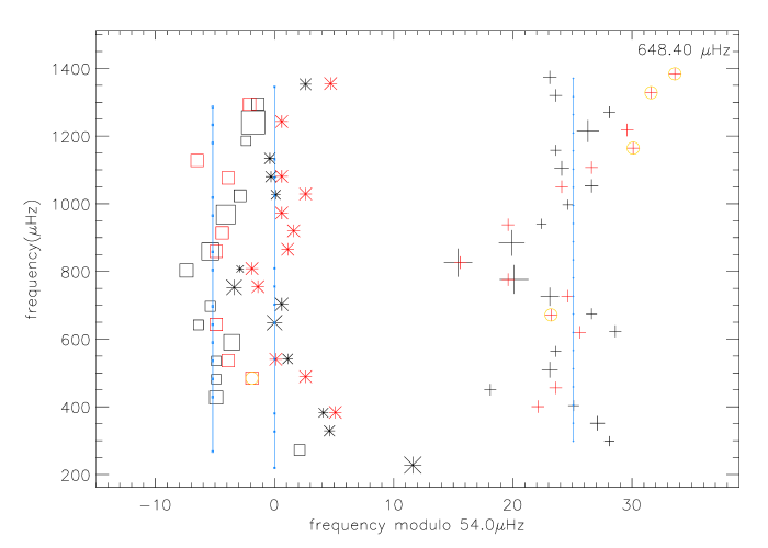
Figure 8: Echelle diagram of the identified modes of degrees $l=0,1,2$ from two-site joint Procyon observations (cf. Table 2). For comparison, we indicate with the symbols in red the frequencies detected from previous OHP/ELODIE 1998 run. Vertical lines correspond to the best fit of the observed frequencies to the asymptotic relation, with $\nu_{0}$=648.4 $\mu$Hz, $\Delta\nu_{0}=53.6\,\mu$Hz and $D_{0}=0.85\,\mu$Hz

Table 2: Mode frequencies of Procyon A (in $\mu$Hz)

$n_{\rm p}$	$l=2\,(n_{\rm p}\,-\,1)$	$l=0$	$l=1$
-10	272.5 (273.9)	(278.)	299.
-9		329.	352.
-8		382.	(400.8) 403.5
-7	427.5		450.5 (456.6)
-6	481.5	(484.)	(507.6) 509.7
-5	535.5	541.3	564.6 (568.)
-4	590.8	(596.)	(619.) 623.
-3	642.	648.4	(671.6) 675.
-2	697.	702.6	725.5 (726.3)
-1	(749.6)	753.	776.7
n0	803.	807.3	825.5 or 834.5
+1	859.1		884.5
+2	(908. 910.)		941.
+3	(964.) 968.		997.
+4	(1021.) 1023.5	1026.5	1050.5 (1052.3)
+5	(1076.5)	1080.	1104.5
+6	(1130.)	1134.	1158.
+7	1186.	(1190.)	(1214.5)
+8	1241.	(1244.6)	1270.
+9	1295.		1320.8 (1328.)
+10		1353.	1373. (1384.)

We list in Table 2 the frequencies of identified modes, detected more than once in different data sets. Some of the frequencies, marked in parenthesis, are detected in longer sequences with better resolution but with a more complicated window function (see Table 1). In higher frequency ranges, two pairs of peaks (1320.8, 1373 and 1328, 1384 $\mu$Hz) are recurrent in different subsets of the data at the $3\,\sigma$ level above the noise and can be equally identified as $l=1$ modes or aliases. Note that at the frequencies of the second pair, the modes would follow an important curvature in the echelle diagram.

6 $p$-mode analysis

Different combinations of frequencies of low degree $p$-modes carry information on different parts the of the stellar structure. The large separation between frequencies of modes of given degree $l$ and consecutive radial orders is sensitive to the global structure and depends on the outer layers of the star. It is mainly related to the stellar radius or the dynamical frequency $\propto(GM/R^{3})^{0.5}$. Mean separations between frequencies of modes with degree, $l,l+2$ or $l,l+1$, which penetrate differently in the central layers, are mainly sensitive to the structure of the deep interior and hence to the evolutionary state. From different models of Procyon by Provost et al. (2002), in the range of considered stellar parameters and overshoot parameters, the mean small spacings $\delta\nu_{02}$, $\delta\nu_{01}$, $\delta\nu_{13}$ vary respectively within $1\,\mu$Hz, $1.5\,\mu$Hz and $2\,\mu$Hz. Such small differences are difficult to measure with the precision of our data.

Figure 9: Variation of the large spacing between the modes of same degree, compared to the predicted curve from the standard model for $l=0$ (Chaboyer et al. 1999). The observed average large separations for $l=0,1,2$ degree are indicated by the horizontal lines.

In Fig. 9, we show the large separation as a function of frequency, for $l=0,1,2$. Note that the mean large spacing does not depend much on the degree. When the successive orders are not detected, the separation was calculated by linear interpolation. Few mode frequencies are dispersed more than $\pm\,2\,\mu$Hz around the mean separations. One of the strongest peaks at $825\pm\,2\,\mu$Hz, identified as the $l=1$ mode is eventually displaced by an avoided crossing (see e.g., Audard et al. 1995; Di Mauro et al. 2003), but additional data are needed to confirm this possibility.

Considering the small spacing of about only $4\,\mu$Hz above 0.7 mHz, it is rather difficult with the present data to distinguish without ambiguity $l=0$ from $l=2$ modes of successive radial order. We should however note that the number of identified $l=2$ modes is higher than for $l=0$. The observed larger amplitude of these modes is probably due to interferences between modes of different $m$. To estimate the rotational splitting of the modes we assumed uniform rotation and the inclination of the rotational axis equal to the inclination of the orbital axis of the binary system ($31.1^{\circ}$) determined by Girard et al. (2000). With an estimated radius of $2.071\,R_{\odot}$ and $v$sin$i$ between 2.7 km/s (Prieto et al. 2002) and 6.1 km/s (Pijpers 2003) the corresponding rotational splitting is respectively 0.58 and $1.3\,\mu$Hz. We performed several simulations (cf. section 3) in which synthetic oscillation spectra are computed with the rotational frequency between these two values. As verified with simulations for a given rotational splitting a pair of $l=0,2$ modes may overlap and produce one single large peak at shifted frequency in the power spectrum. The frequency resolution of joint OHP and AFOE data is not sufficient to attempt a determination of rotational splitting.

7 Oscillation amplitudes

Based on Christensen-Dalsgaard & Frandsen (1983) computations of expected amplitudes from stochastic excitation in stars on or near the main sequence, Kjeldsen & Bedding (1995) proposed a scaling for the oscillation velocity amplitude $V_{\rm osc}\propto\,L/M$ , where L is the luminosity and M the mass of the star. The calculations by Houdek et al. (1999) confirmed this result, although they fitted better the velocity with $V_{osc}\propto\,(L/M)^{s}$, and $s\sim 1.5$. However, both the simple scaling law and the computation of Houdek et al. grossly overestimate the observed amplitudes of Procyon ($\lesssim\,50$ cm/s).

To reduce the ”expected” amplitude of Procyon, Kjeldsen & Bedding (2001) suggested that $V_{\rm osc}$ is independent of the effective temperature amongst stars of a given $M$ and radius $R$. They proposed $V/V_{\sun}\propto\,g_{\sun}/g$ (g surface gravity) which, for Procyon, yields lower velocity ($70$ cm s^-1) than the scaling $V/V_{\sun}=2[(g_{\sun}/g)^{0.6}+(g_{\sun}/g)^{4.5}]^{-1}$ (Gilliland et al. 1993), but still higher than the observations.

Theoretical amplitudes from models are also overestimated, almost three times higher than the observed one. It appears (Houdek & Gough 2002), therefore, that there is something wrong with the theory of the pulsations or the convection, or their coupling, for this relatively hot and luminous star. According to Houdek (2002), for solar-type stars hotter than the Sun and with masses $M\,>\,1.35\,M_{\sun}$, theoretical damping rates may be too small and estimated convective velocities too large, leading to predicted amplitudes larger than the data suggest.

We note however that the same scaling as in the solar case, $\nu_{\rm max}\sim 0.6\,\nu_{\rm ac}$ where the acoustic cutoff frequency $\nu_{\rm ac}\propto\,g\,T_{\rm eff}^{-1/2}$ (Brown et al. 1991), can be used to obtain a good agreement for the frequency at which the oscillation amplitudes are largest. Using a recent value for the T${}_{\rm eff}=6530$ K from Prieto et al. (2002), yields $\nu_{\rm ac}\sim\,1.7\,\mu$Hz and $\nu_{\rm max}\sim\,956\,\mu$Hz.

8 Conclusions

Two-site observations of Procyon A confirmed the presence of solar-like oscillations, characterized by a large frequency separation $\Delta\nu_{0}=(53.6\,\pm\,0.5)\mu$Hz. We identified 45 $p$-modes frequencies in the range $300\,-\,1400\,\mu$Hz with harmonic degrees $l=0,1,2$, in good agreement with the theoretical predictions by Chaboyer et al. (1999). The significative departure of the modes in the region of the maximum oscillation amplitudes from the asymptotic relation explains the difficulties in finding the mean principal frequency separation $\Delta\nu_{0}$ and the small frequency separation $\delta\nu_{02}$ by usual techniques based on the best fit of the asymptotic relation from an $l$-mixed analysis. Additional data with higher frequency resolution are needed to determine the rotational splitting and the damping time of Procyon p-modes. By determining oscillation frequencies with an accuracy better than $0.5\,\mu$Hz from an extended ground-based multi-site campaign on Procyon we will be able to test the techniques for the mode detection and prepare the scientific exploitation of future asteroseismic observations from space (MOST, COROT, EDDINGTON).