A General Relativistic Magnetohydrodynamic Simulation of Jet Formation

Abstract

We have performed a fully three-dimensional general relativistic magnetohydrodynamic (GRMHD) simulation of jet formation from a thin accretion disk around a Schwarzschild black hole with a free-falling corona. The initial simulation results show that a bipolar jet (velocity $\sim 0.3c$) is created as shown by previous two-dimensional axisymmetric simulations with mirror symmetry at the equator. The 3-D simulation ran over one hundred light-crossing time units ($\tau_{\rm S}=r_{\rm S}/c$ where $r_{\rm S}\equiv 2GM/c^{2}$) which is considerably longer than the previous simulations. We show that the jet is initially formed as predicted due in part to magnetic pressure from the twisting the initially uniform magnetic field and from gas pressure associated with shock formation in the region around $r=3r_{\rm S}$. At later times, the accretion disk becomes thick and the jet fades resulting in a wind that is ejected from the surface of the thickened (torus-like) disk. It should be noted that no streaming matter from a donor is included at the outer boundary in the simulation (an isolated black hole not binary black hole). The wind flows outwards with a wider angle than the initial jet. The widening of the jet is consistent with the outward moving torsional Alfvén waves (TAWs). This evolution of disk-jet coupling suggests that the jet fades with a thickened accretion disk due to the lack of streaming material from an accompanying star.

1 Introduction

Relativistic jets have been observed in active galactic nuclei (AGNs) (e.g. Urry & Pavovani 1995; Ferrari 1998; Blandford 2002), in microquasars in our Galaxy (e.g. Mirabel & Rodriguez 1999), and it is believed that they originate in the regions near accreting (stellar) black holes and neutron stars (Meier, Koide, & Uchida, 2001). To investigate the dynamics of accretion disks and the associated jet formation, we have performed jet formation simulations using a full 3-D GRMHD code. This magnetic-acceleration mechanism has been proposed not only for AGN jets, but also for (nonrelativistic) protostellar jets (see Meier, Koide, & Uchida (2001)). Kudoh, Matsumoto, & Shibata (1998) found that the terminal velocity of a jet is comparable to the rotational velocity of the disk at the foot of the jet in nonrelativistic MHD simulations, and that a relativistic jet should be formed near the event horizon. It should be noted that the mechanism of jet generation in neutron star binaries may be different from black hole binaries. Recently, an ultra-relativistic outflow was observed from an accreting stellar-mass neutron star (Fender et al. 2004). Fender et al. (2004) have concluded that the generation of highly relativistic outflows does not require properties unique to black holes, such as an event horizon. It seems plausible that production of ultrarelativistic jets may be a generic feature of accretion onto neutron stars such as Cir-X and Sco X-1 at or near to the Eddington limit. This result differs from the suggestions that the velocities of jets would be limited to the surface escape speed (Livio 1999).

The fluorescent iron line (K_α) seen in the X-ray spectrum of many active galactic nuclei (AGNs), and particularly in Seyfert galaxies, has provided us with an extremely useful probe of the region close to an accreting black hole. This is an important diagnostic with which to study Doppler and gravitational redshifts, thereby providing key information on the local kinematics of the material (see the reviews by Fabian et al. 2000 and Reynolds & Nowak 2003). The simultaneous X-ray/IR flares from a black hole/relativistic jet system are the observational evidence revealing a time-dependent interaction between the jet and inner disk (e.g. Ueda et al. 2002). In regions where disk-jet interactions take place near a black hole, the plasma and magnetic fields interact in a complicated manner; therefore a 3-dimensional GRMHD simulation such as we perform here is required to investigate dynamics near the horizon and ultimately to couple predicted dynamics to the iron line.

Koide, Shibata, & Kudoh (1999) have investigated in 2-D, the dynamics of an accretion disk initially threaded by a uniform magnetic field in a non-rotating corona (either in a state of steady fall or in hydrostatic equilibrium) around a non-rotating (Schwarzschild) black hole. The numerical results show that matter in the disk loses angular momentum by magnetic braking, then falls into the black hole. The disk falls faster in this simulation than in the non-relativistic case because of general-relativistic effects that are important below $3r_{\rm S}$, where $r_{\rm S}\equiv 2GM/c^{2}$ is the Schwarzschild radius. A centrifugal barrier at $r=2r_{\rm S}$ strongly decelerates the infalling material. Plasma near the shock at the centrifugal barrier is accelerated by the ${\bf J}\times{\bf B}$ force and forms bipolar jets. Inside this magnetically driven jet, the gradient of gas pressure also generates a jet above the shock region (gas-pressure driven jet). This two-layered jet structure is formed both in a hydrostatic corona and in a steady-state falling corona. Koide et al. (2000) have also developed a new GRMHD code using a Kerr geometry and have found that, with a rapidly rotating ($a\equiv J/J{\max}=0.95$, $J_{\max}=GM^{2}/c$, $J$ and $M$ are angular momentum and mass of black hole) black-hole magnetosphere. the maximum velocity of the jet is (0.3 - 0.4) $c$. Recently the extraction of rotational energy from plasma in the ergosphere has been investigated (Koide et al. 2002; Koide 2003). All of these GRMHD simulations were made assuming axisymmetry with respect to the $z$-axis and mirror symmetry with respect to the plane $z=0$. It is known that the axisymmetric assumption suppresses azimuthal instabilities.

Magnetic fields are expected to play an essential role in the dynamics of most relativistic objects such as active galactic nuclei, X-ray binaries, gamma-ray bursts, and quasars. In accretion disks, the most important role of the magnetic field is angular momentum transport, which twists the field, and results in torsional Alfvén waves (TAWs) and associated jet formation (Koide et al. 1999). Based on the importance of magnetorotational instability (MRI) in accretion disks (Balbus & Hawley, 1998), the nonlinear growth of these instabilities has been investigated by three-dimensional global MHD simulations of black hole accretion disks (Hawley, 2000; Igumenshchev, Abramowicz, & Narayan, 2000; Hawley, 2001; Hawley & Krolik, 2001; Machida, Hayashi, & Matsumoto, 2000; Hawley, Balbus, & Stone, 2001; Armitage, Reynolds, & Chiang, 2001; Reynolds & Armitage, 2001; Hawley & Krolik, 2002; Hawley & Balbus, 2002; Krolik & Hawley, 2002; Machida & Matsumoto, 2003; Igumenshchev, Narayan, & Abramowicz, 2003) using a pseudo-Newtonian potential (Paczyńsky & Witta, 1980). Machida & Matsumoto (2003) investigated black hole accretion flow using three-dimensional global resistive MHD simulations. They conclude that the reconnection in the innermost region releases enough energy to explain the origin of X-ray bursts from black hole candidates.

Recently, more GRMHD simulations have been developed by De Villiers & Hawley (2002, 2003a); Gammie, McKinney, & Tóth (2003). In particular, Gammie, McKinney, & Tóth (2003) have employed the numerical scheme HARM (High Accuracy Relativistic Magnetohydrodynamics) in which the conservation schemes for GRMHD are used (Koide, Shibata, & Kudoh, 1998, 1999; Koide et al., 2000). A nonconservative scheme for GRMHD following a ZEUS-like approach has been developed also by De Villiers & Hawley (2002). They also compare the code performance of 1-D and 2-D test cases. De Villiers & Hawley (2003b) have investigated the properties of accretion flows with tori in the Kerr metric using 3-D GRMHD simulations. The MRI in torus has also been investigated using Schwarzschild and Kerr metrics (De Villiers, Hawley, & Krolik 2003; Hirose, et al. 2004, De Villiers, et al. 2004; Krolik, Hawley, & Hirose 2004).

Different studies have chosen various initial magnetic fields. We have chosen an initial magnetic field from the Wald’s exact analytic solution for a Kerr black hole immersed in a uniform magnetic field (Wald 1974; Punsley 2001; Komissarov 2004). De Villiers, Hawley & Krolik (2003) have performed simulations in which the initial conditions for the accretion disks and magnetic fields are appropriate for MRI research. They have investigated the properties of accretion flows in the Kerr metric including bi-conical outflows in the quarter sphere with periodic boundary conditions in the azimuthal direction. These simulations use the torus accretion disks as an initial condition. The inner edge of the accretion disk is located at $r=15r_{\rm S}$, and the inner edge moves into the innermost stable radius within one orbit (De Villiers, Hawley, & Krolik 2003). In these simulations, the initial field consists of axisymmetric (azimuthal) field loops, laid down along an isodensity surface within the torus, which is different from the initial uniform magnetic field used in simulations by Koide, Shibata, & Kudoh (1999) and Nishikawa et al. (2002, 2003). The initial weak loop magnetic fields contribute to the generation of the MRI and the associated jet. However, the structure of magnetic fields piled up near the black hole in their simulations is different from the magnetic fields which are twisted and pinched (not wound) by the free-falling corona and accretion disk (Koide, Shibata, & Kudoh 1998, 1999; Koide et al. 2000; Nishikawa et al. 2002, 2003). The absence of a free-falling corona (Bondi & Hoyle 1944; Bondi 1952; Michel 1972) as well as the initial loop magnetic field in (De Villiers, Hawley & Krolik 2003) results in different dynamics of the accretion disk and associated jet formation, compared to the case with the free-falling corona and initial uniform magnetic field in Koide, Shibata, & Kudoh (1999) and Nishikawa et al. (2002, 2003).

In this paper we present a fully three-dimensional, GRMHD simulation of jet formation with a thin accretion disk. Our motivation for this type of simulation is to determine the parameters necessary for relativistic jet formation and the resulting interaction and instabilities found between the accretion disk and the black hole. The simulation we present here was performed using the same parameters as in Koide, Shibata, & Kudoh (1999) in order to determine the physical differences resulting from a full 3-D versus a 2-D simulation with axisymmetry and mirror symmetry at the equator. The three-dimensional simulation allows us to study the evolution of jet formation because it is run for longer light-crossing times than the previous two-dimensional simulations. We find that at the later stages of the simulation the accretion disk becomes thick and a wind is formed with a much wider angle than the collimated jet formed at the earlier stage. In Section 2, we describe the governing GRMHD equations. The simulation model and numerical method is described in Section 3. Our new simulation results are presented in Section 4 followed by a summary and discussion in Section 5.

2 3-D GRMHD Governing Equations and Numerical Approach

The governing equations for GRMHD are written in conservation form based on Weinberg (1972) and Misner, Thorne, & Wheeler (1973). Four-dimensional space-time parameters are written with Greek indices, while Latin indices are used for three-dimensional space, $x^{\alpha}=(ct,x^{j})$. The physical parameters include, four-velocity ($U^{\alpha}$), proper density ($\rho$), proper pressure ($p$), adiabatic index ($\Gamma$), and proper internal energy density ($e_{\rm int}\equiv\rho c^{2}+p/(\Gamma-1)$). Relativistic parameters include the Christoffel symbols ($\Gamma^{\alpha}_{\beta\gamma}$) and metric terms ($g_{\alpha\beta}$). The pressure is related to the other variables by the equation of state, $p\propto\rho^{\Gamma}$. The specific relativistic enthalpy is given by, $h=e_{\rm int}+p=\rho c^{2}+\Gamma p/(\Gamma-1)$.

The conservation equations are derived from the continuity equation, $\nabla_{\gamma}\left(\rho U^{\gamma}\right)=0$, and the conservation of the stress energy tensor, $\nabla_{\mu}T^{\mu\upsilon}=T^{\mu\upsilon}_{;\mu}=T^{\mu\upsilon}_{,\mu}+T^{\alpha\upsilon}\Gamma^{\mu}_{\alpha\mu}+T^{\mu\alpha}\Gamma^{\upsilon}_{\alpha\mu}=0$. From Maxwell’s equations, the electromagnetic field-strength tensor is denoted by $F_{\alpha\beta}=\partial_{\alpha}A_{\beta}-\partial_{\beta}A_{\alpha}$ and the four-current density by $J^{\beta}$, where $A_{\alpha}$ is the four-vector potential. The Maxwell equations are written $\partial_{\mu}F_{\alpha\beta}+\partial_{\alpha}F_{\beta\mu}+\partial_{\beta}F_{\mu\alpha}=0$ and $\nabla_{\alpha}F^{\alpha\beta}=-J^{\beta}$.

For the simulation in the context of this paper, we have assumed infinite electric conductivity, $F_{\alpha\beta}U^{\alpha}=0$. The stress energy tensor ($T^{\alpha\beta}$) for an ideal fluid in an electromagnetic field and in a general relativistic environment is,

$$T^{\alpha\beta}=\left(\rho+p\frac{\Gamma}{\Gamma-1}\right)U^{\alpha}U^{\beta}+pg^{\alpha\beta}+F^{\alpha}_{\sigma}F^{\beta\sigma}-g^{\alpha\beta}\frac{F^{\lambda\gamma}F_{\lambda\gamma}}{4}.$$ (1)

We assume that the off-diagonal spatial elements of the metrics $g_{\mu\nu}$ vanish: $g_{ij}=0\,(i\neq j)$. Here Roman indeces ($i,j$) run from 1 to 3, the

$$g_{00}=-h_{0}^{2},\;\;\;g_{ii}=h_{i}^{2},\;\;\;g_{i0}=g_{0i}=-h_{i}^{2}\omega_{i}/c,$$ (2)

The line element is written

$$ds^{2}=-\alpha^{2}(cdt)^{2}+\sum_{i=1}^{3}(h_{i}dx^{i}-c\beta^{i}\alpha dt)^{2}.$$ (3)

Here, the lapse function and shift velocity are defined by $\alpha=\sqrt{h^{2}_{0}+\sum_{i=1}^{3}(\frac{h_{i}\omega_{i}}{c})^{2}}$ and $\beta^{i}=\frac{h_{i}\omega_{i}}{c\alpha}$, respectively.

The 3 $+$ 1 form of equations are employed (Weinberg 1972; Thorne, Price, & Macdonald 1986). The 3 $+$ 1 set of equations used in these simulations for the general relativistic conservation laws governing the plasma and Maxwell equations were derived in Koide, Shibata, & Kudoh (1999) and Koide (2003). The detailed presentation of the equation is provided in Koide (2003) and will not be repeated here. The numerical scheme is constructed in the set of conservation variables $D{\rm(density)},P^{i}{\rm(momentum)},\epsilon$ (energy), and $B^{i}$ (for details see Koide, Shibata, & Kudoh (1999) and Koide (2003)). The values of the primitive variables ${\bf v}$, $\rho$, Lorentz factor, and $p$ are calculated from $D,P^{i},\epsilon$, and $B^{i}$. Two nonlinear, simultaneous algebraic equations with unknown variables, $a\equiv\gamma-1$ and $b\equiv\gamma({\bf v}\cdot{\bf B})/c^{2}$, are solved using a two variable Newton-Raphson iteration method (for details see Koide, Shibata, & Kudoh (1999) and Koide (2003)). Here the Lorentz factor is defined $\gamma=1/\root \of{(1-\sum_{i=1}^{3}(v^{i}/c)^{2})}$.

In the course of the simulation, Gauss’s law for the magnetic field, $\nabla\cdot{\bf B}=0$, and the charge conservation law, $\nabla_{\mu}{\bf J}^{\mu}=0$ must be verified. Here, ${\bf J}^{\mu}=(c\rho_{\rm c},J^{1},J^{2},J^{3})$ is the current four vector. We adapt the Boyer-Lindquist coordinate system ($t,r,\theta,\phi$), the metric of Schwarzschild space-time is simplified to

$$h_{0}=\alpha,\;\;\;h_{1}=1/\alpha,\;\;\;h_{2}=r,\;\;\;h_{3}=r\sin\theta,\;\;\;\omega_{i}=0$$ (4)

where the lapse function is $\alpha=(1-r_{\rm S}/r)^{1/2}$ and Schwarzschild radius is $r_{\rm S}=2GM/c^{2}$ (${\rm G}=6.67\times 10^{-11}$ Nm${}^{2}/$kg² is the gravitational constant). Here, $r,\,\theta,\,\phi$ are radial, latitudinal, and azimuthal coordinates, respectively. The line element for the Schwarzschild metric has the form

$$ds^{2}=-\left(1-\frac{r_{\rm S}}{r}\right)c^{2}dt^{2}+\left(1-\frac{r_{\rm S}}{r}\right)^{-1}dr^{2}+r^{2}d\theta^{2}+r^{2}\sin^{2}\theta d\phi^{2}.$$ (5)

We use the modified tortoise radial coordinate, $r^{\prime}={\rm ln}(r/r_{\rm S}-1)$.

The GRMHD equations described in this section, with the applied initial and boundary conditions (which will be described in the next section), were solved using the simplified total variation diminishing (TVD) method. The simplified TVD method was developed by Davis (1984) for studying violent phenomena such as shocks (Koide, Nishikawa, & Mutel 1996; Nishikawa et al. 1997, 1998; Koide, Shibata, & Kudoh 1999). This method stems from Lax-Wendoroff’s method, with additional diffusion terms. It was verified in Koide, Shibata, & Kudoh (1999) that this method obeys the laws of conservation of energy. The conservation laws ($\partial\rho_{e}/\partial t+\nabla\cdot\alpha(J+\rho_{e}c\beta)=0$), where $\alpha$ and $\beta$ is lapse function and shift vector, respectively. is restraint almost zero within the round-off error with the double precision. It was also confrmed that when we take the nonrelativistic limit ($(v/c)^{2}\ll 1$), the Newtonian calculation (nonrelativistic MHD simulation) of a magnetized jet resulted (Koide, Nishikawa, & Mutel 1996).

3 3-D GRMHD Simulations: Simulation Parameters and Numerical Techniques

In this section we present our results showing the fully three dimensional simulations of jet formation using general relativistic magnetohydrodynamics. In the assumed initial state of our simulations, the region is divided into two parts: a background corona surrounding the black hole, and an accretion disk along the equatorial plane of the geometry (see Fig. 1a). The simulation results are displayed in the Cartesian coordinate transforming from the Boyer-Lindquist coordinates ($t,\,r,\,\theta,\phi$) coordinate ($x=r\sin\theta\cos\phi,y=r\sin\theta\sin\phi,z=r\cos\theta$). The black hole is located at the origin ($x=y=z=0$). The coronal plasma is set in a state of transonic free-fall flow (Bondi accretion), with an adiabatic exponent, $\Gamma=5/3$, specific relativistic enthalpy, $h=1.3$, and sonic point located at $r=1.6r_{\rm S}$. The Keplerian disk region is located at $r>r_{\rm D}\equiv 3r_{\rm S},|{\rm cos}\theta|<\delta,$ where $\delta=1/8$, $r_{\rm D}$ is the disk radius and $r_{\rm S}$ the Schwarzschild radius. In this region the density is 100 times that of the background corona, while the orbital velocity, $v_{\phi}$, is relativistic and purely azimuthal: $v_{\phi}=v_{\rm K}\equiv c/[2(r/r_{\rm S}-1)]^{1/2}$, where $v_{\rm K}$ is the Keplerian velocity. (Note that this equation reduces to the Newtonian value, $v_{\rm\phi}=\sqrt{GM/r}$, in the non-relativistic limit $r_{\rm S}/r\ll 1$). The pressure of both the corona and the disk are assumed to be equal to that of the transonic solution. The initial conditions for the plasma surrounding the black hole in terms of the transonic flow velocity, density and pressure ($v_{\rm ffc},\rho_{\rm ffc},p_{\rm ffc}$) and the disk properties ($v_{\rm dis},\rho_{\rm dis},p_{\rm dis}$) are:

$$\rho=\rho_{\rm ffc}+\rho_{\rm dis}$$ (6)

$$\rho_{\rm dis}=\left\{\begin{array}[]{cc}100\rho_{\rm ffc}&\verb! !(r>r_{\rm D}\verb! !{\rm and}\verb! !|{\rm cot}\theta|<\delta)\\ 0&\verb! !(r\leq r_{\rm D}\verb! !{\rm or}\verb! !|{\rm cot}\theta|\geq\delta)\end{array}\right.$$ (7)

$$(v_{r},v_{\theta},v_{\phi})=\left\{\begin{array}[]{cc}(0,0,v_{\rm K})&\verb! !(r>r_{\rm D}\verb! !{\rm and}\verb! !|{\rm cot}\theta|<\delta)\\ (-v_{\rm ffc},0,0)&\verb! !(r\leq r_{\rm D}\verb! !{\rm or}\verb! !|{\rm cot}\theta|\geq\delta)\end{array}\right.$$ (8)

where we set $\delta=0.125$ and the smoothing length is $0.3r_{\rm S}$. The initial conditions for the free-falling corona are based on theories by Bondi & Hoyle (1944), Bondi (1952), and Michel (1972).

An initially uniform magnetic field is applied perpendicular to the accretion disk. It is set to the Wald solution (Wald 1974), which represents the uniform magnetic field around a Schwarzschild black hole; $B_{r}=B_{0}{\rm cos}\theta$ and $B_{\theta}=-\alpha B_{0}{\rm sin}\theta$ (where $\alpha$ is the lapse function defined in section 2). At the inner edge of the accretion disk, the proper Alfvén velocity is $v_{\rm A}=0.015c$ when $B_{0}=0.3\,\root \of{\rho_{0}c^{2}}$. The Alfvén velocity in the fiducial observer frame is

$$v_{\rm A}\equiv\frac{B}{\root \of{\rho+[\Gamma p/(\Gamma-1)+B^{2}]/c^{2}}}.$$ (9)

The plasma beta of the corona, which is defined as the ratio of gas pressure to magnetic pressure, is: $\beta\equiv p/(B^{2}/2)=1.40$ at $r=3r_{\rm S}$. The sound speed is calculated from $v_{\rm S}\equiv c(\Gamma p/h)^{1/2}$. Our simulation domain is, $1.1r_{\rm S}\leq r\leq 20r_{\rm S}$, $0\leq\theta\leq\pi$, $0\leq\phi\leq 2\pi$, with a mesh size of $100\times 60\times 120$. The effective linear mesh spacing at $r=1.1r_{\rm S}$ and at $r=20r_{\rm S}$ is $5.38\times 10^{-3}r_{\rm S}$ and $0.97r_{\rm S}$, respectively. The angular spacing along the polar and azimuthal directions is $5.2\times 10^{-2}$ rad. At the $z$-axis ($\theta=0,\;\pi$) the fixed boundary is used, therefore the kink instability is suppressed near the axis. (However, a warping instability near the equator is not suppressed.) The following radiative boundary condition is imposed at $r=1.1r_{\rm S}$ and at $r=20r_{\rm S}$:

$$u_{0}^{n+1}=u_{0}^{n}+u_{1}^{n+1}-u_{1}^{n},$$ (10)

where the superscript $n$ denotes the time step, the subscript 0 refers to the boundary node, and the subscript 1 is the node neighboring the boundary. The computations were done on an SGI ORIGIN 2000 system with 0.898 GB of internal memory. 47 hours of CPU time were needed for 10,000 time steps.

Contributions to jet formation from the gas pressure and electromagnetic field components are found using the following equations derived in Koide, Shibata, & Kudoh (1999):

$$W_{gp}\equiv-{\bf v}\cdot\nabla p$$ (11)

$$W_{EM}\equiv{\bf v}\cdot\left({\bf E}+{\bf J}\times{\bf B}\right)$$ (12)

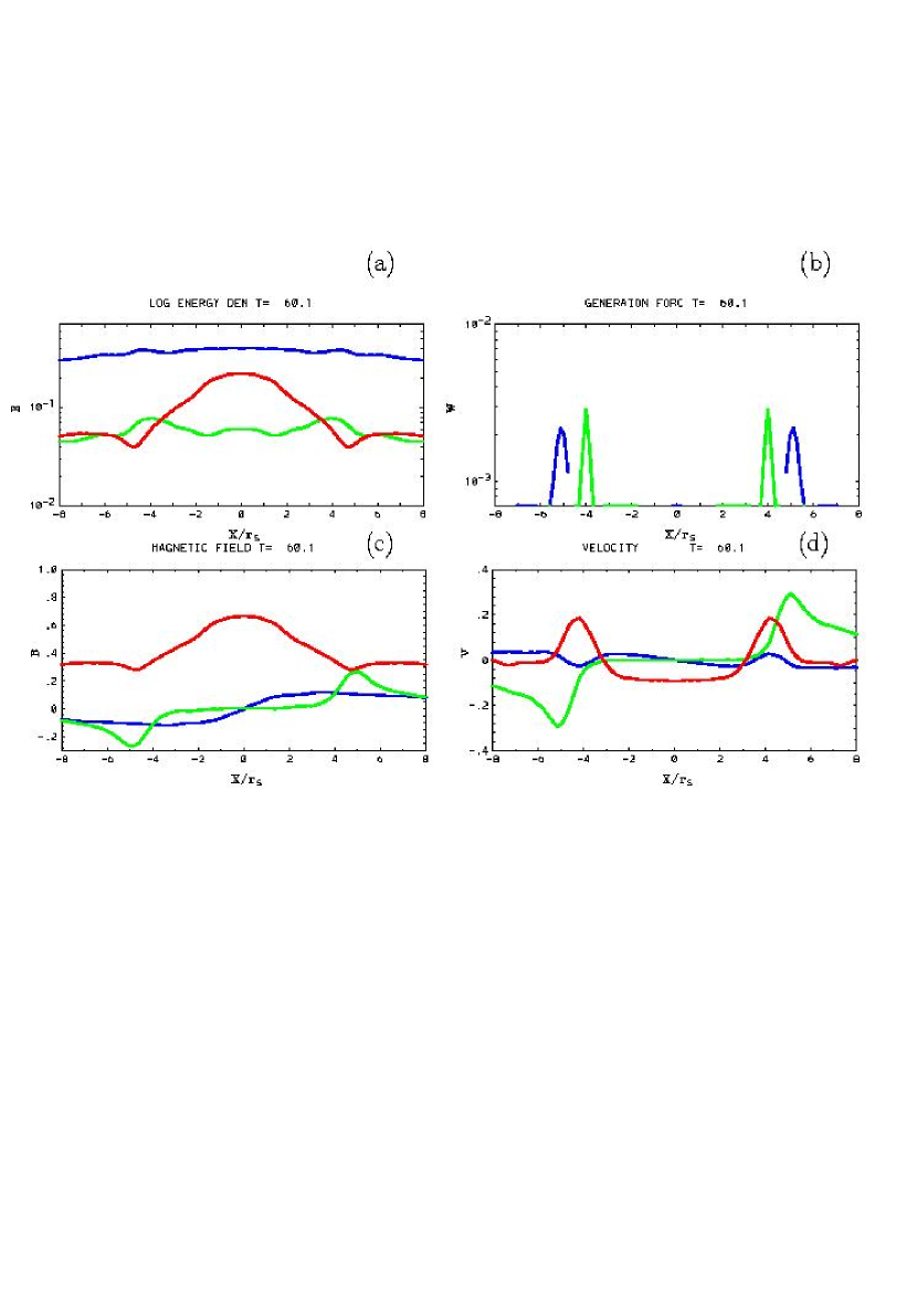
Figure 6: This plot represents various physical quantities on the $z=5.6r_{\rm S}$ surface at $t=60.0\tau_{\rm S}$. Frame (a) shows the values for proper mass density $\rho$ (blue), proper pressure $p$ (green) and z component magnetic field energy $B^{2}_{\rm z}/2$ (red). Frame (b) is the power contribution from the pressure, $W_{\rm gp}$ (green) and the electromagnetic force, $W_{\rm EM}$ (blue). We can find the two-layer acceleration region in the jet. Frame (c) shows the individual magnetic field components $B_{\rm x}$ (blue), $B_{\rm y}$ (green), and $B_{\rm z}$ (red). Frame (d) has the components of velocity $v_{\rm x}$ (blue), $v_{\rm y}$ (green), and $v_{\rm z}$ (red).

These equations will be used for showing the energy sources for generating the jet in Figs. 6b and 7b.

4 Simulation Results: Jet Formation

The evolution of jet formation for the simulation performed in the region previously described ($1.1r_{\rm S}\leq r\leq 20r_{\rm S}$, $0\leq\theta\leq\pi$, and $0\leq\phi\leq 2\pi$ with a grid resolution of $100\times 60\times 120$) is shown in Figure 1. The physical values calculated in spherical coordinates are transformed to Cartesian coordinates to display their values (for only limited region near the black hole ($|x|,|y|,|z|\leq 8r_{\rm S}$). The black hole is located at the origin ($x=y=z=0$). The parameters used in this simulation are the same as those of the axisymmetric simulations shown in Fig. 6 of Koide, Shibata, & Kudoh (1999). Figure 1 shows the evolution of the proper density on a logarithmic scale (colored shading) with the flow velocity (shown by the directional arrows) in the $x-z$ plane ($y=0$). The maximum values are normalized for all panels. The black circle represents the black hole’s Schwarzschild radius. Figure 1a presents the initial conditions described in Section 3. Figure 1b ($t=39.2\tau_{\rm S}$) shows that a shock forms in the region of $x=3.5r_{\rm S}$. This shock is due to the rapidly infalling material reaching the centrifugal barrier located at $x=2r_{\rm S}$. At this time, the initial signs of jet formation are seen. When the simulation reaches $t=60.0\tau_{\rm S}$ (Fig. 1c), the jet structure is clearly seen. The formed jet is identified by higher density (Fig. 1c) and pressure (Fig. 2c) along the vertical line at $x=\pm 4r_{\rm S}$. The arrows show the velocity of the jet. This phenomenon was also seen in previous three-dimensional simulations (Nishikawa at al. 2002, 2003). In the last frame (Fig. 1d) at $t=128.9\tau_{\rm S}$, the accretion disk has thickened and the jet appears to fade into a weak wind that flows near the accretion disk. Symmetry at the equator is seen as expected even with the freedom of the three-dimensional simulation as no asymmetric perturbation has been applied.

The proper pressure, over the same time scale, is shown in Figure 2. The jet forms in the shape of a hollow cylinder which is shown clearly in this figure. The pressure in this region is high due to the shock and adiabatic heating at the boundary of the decelerated flow. This high pressure contributes greatly to the jet formation (see Equation 11), which is shown by the green curves in Figs. 6b and 7b. A bi-conical high pressure region with velocity arrows directed away from the disk in Figure 2c represents a jet. However, at the later time the jet is quenched and the pressure decreases, as the shock disappears at $r=3r_{\rm S}$. Figure 2d shows the faded jet and the wind generated along the disk.

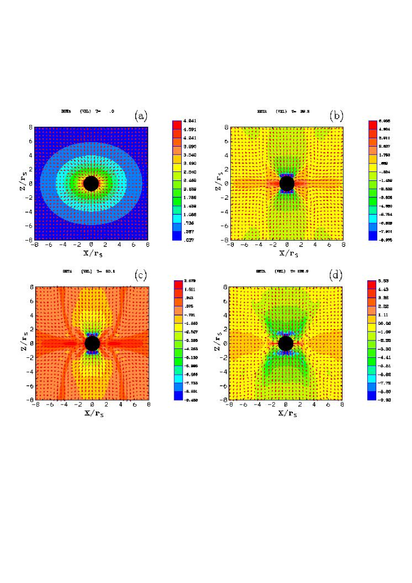
Figure 3: The time evolution of gas to magnetic pressure $\beta=p/(0.5B^{2})$ (color) with velocity arrows at (a) $t=0.0\tau_{\rm S}$, (b) $t=39.2\tau_{\rm S}$, (c) $t=60.0\tau_{\rm S}$, and (d) $t=128.9\tau_{\rm S}$. The profiles of generated jets are seen clearly in Fig. 3c.

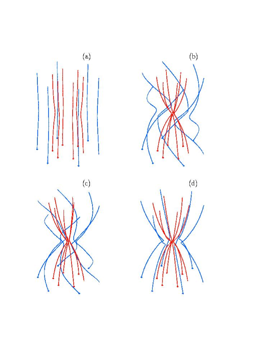
Figure 4: These panels show the time evolution of the magnetic field lines associated with a Schwarzschild black hole and an accretion disk. The field lines are traced from the bottom ($z=-8r_{\rm S}$) with the different radius (red: $r=2.67r_{\rm S}$; blue: $r=5.33r_{\rm S}$) at (a) $t=0.0\tau_{\rm S}$, (b) $t=39.2\tau_{\rm S}$, (c) $t=60.0\tau_{\rm S}$, and (d) $t=128.9\tau_{\rm S}$.

The evolution of the ratio of gas to magnetic pressure $\beta=p/(0.5B^{2})$ in the $x-z$ plane ($y=0$) is shown in Fig. 3. In this figure the maximum and minimum values are not normalized in order to see the relative values at each time. The initial cold accretion disk is heated and the shock is created around $x/r_{\rm S}=\pm 3$ as shown in Fig. 3b. The generated conical jet is seen in Fig. 3c. This structure is also found in tori simulations (Fig. 2 in Hirose et al. (2004)). The jet is ejected along the twisted magnetic field (shown in Fig. 4c). Two layers of high $\beta$ regions are found near the black hole. After the jet is faded, the accretion disk is broadened as seen in Fig. 3d.

The evolution of jet formation is closely related to the deformed magnetic field as shown in Fig. 4. The magnetic field lines, which are initially perpendicular to the accretion disk (Fig 4a), are twisted by the accretion disk as the simulation progresses and are pinched by the falling corona and accretion material (Fig. 4b). Later the disk drags the magnetic field further in the azimuthal direction, transferring angular momentum outward even as matter falls toward the black hole. The pinching twisting field lines increase the magnetic field pressure and generate a jet near the black hole (Fig. 4c). Equation 12 presents the power of the electromagnetic forces which drives jet formation as is also shown by the blue curves in Figs. 6b and 7b. At $t=128.9\tau_{\rm S}$ the magnetic field has relaxed and is consistent with what is seen in Figures 1d and 2d where the jet fades.

Recently, Hirose et al. (2004) have analyzed the magnetic field structures found in 3-D GRMHD simulations of tori in the Kerr metric (De Villiers, Hawley, & Krolik 2003). It should be noted that their different initial magnetic field conditions lead to different magnetic field dynamics. For example, the sample field lines in Fig. 6 in Hirose et al. (2004) for the spin parameter $a/M=0.9$ (even $a/M=0$) are substantially different from the magnetic field lines in Fig. 4. Since the magnetized disk in our model is stable to MRI, the magnetic fields are never tangled. De Villiers et al. (2004) have found the unbound outflows in the axial funnel region, which consist of two components: a hot, fast, tenuous outflow in the axial funnel proper, and a colder, slower, denser jet along the funnel wall.

The time required to form the jet in this three-dimensional simulation is similar to the two-dimensional axisymmetric simulations. Ultimately, we expect that the dynamics of jet formation are modified by the additional coordinate freedom in the azimuthal dimension (when axisymmetry with respect to the $z$-axis is removed), such as the difference between axisymmetric 2-D and full 3-D MHD simulations found by Matsumoto (1999). Due to the growth of non-axisymmetric instabilities, the magnetic field lines were compressed into helical bundles in the jet. In this simulation with a thin disk a global and visible instability was not found in the $x-y$ plane. One of the possible reasons is that the strong magnetic field along the $z$-axis (low $\beta$ value) prevents growth of MRI. The magnetic fields found with MRI are usually along the azimuthal direction (the initial $\beta$ value is larger) (e.g. De Villiers, Hawley, & Krolik 2003).

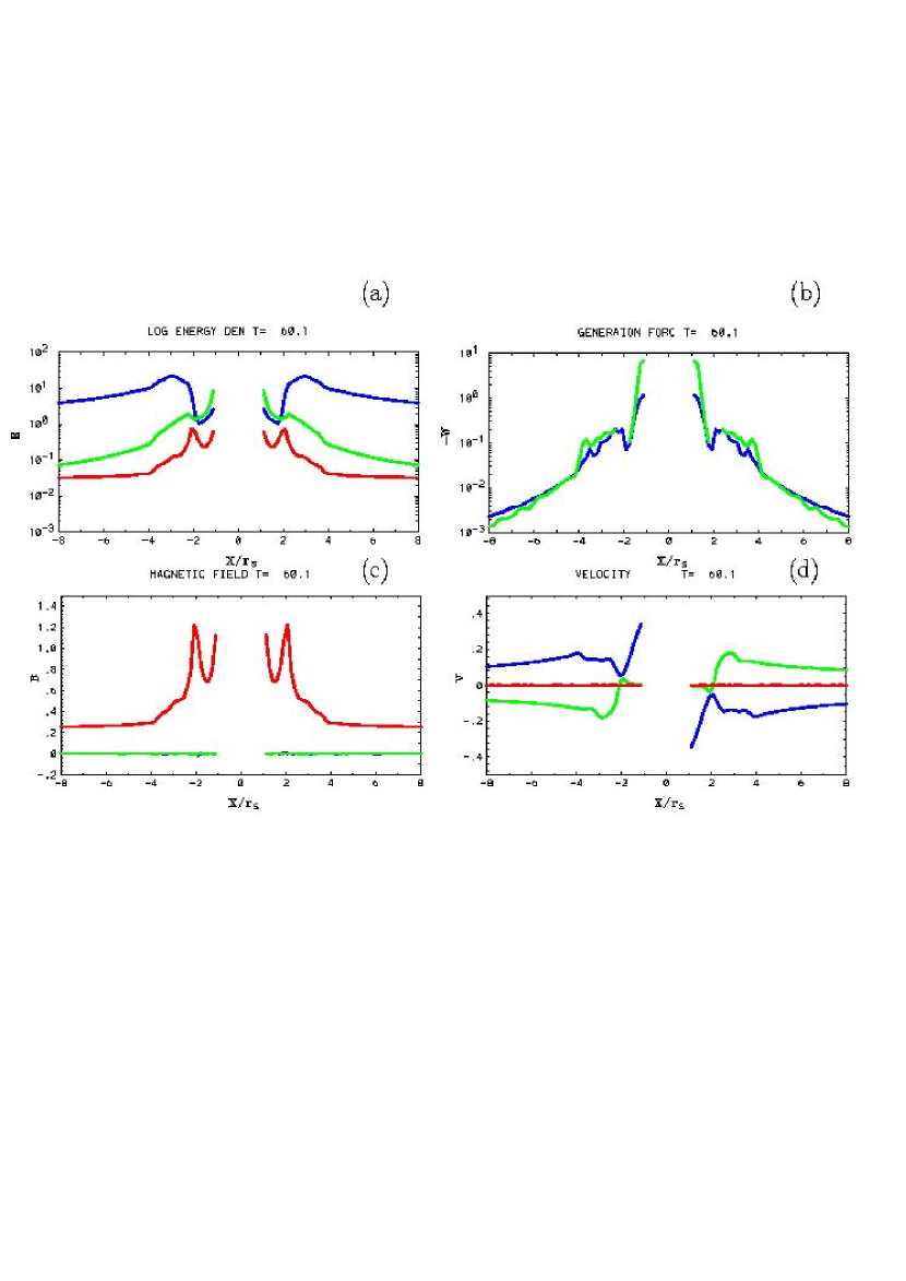
Figure 5: This plot represents the one dimensional slice through the simulation domain at $z=0$ at $t=60.0\tau_{\rm S}$. The location of the black hole is excluded in the plots. Frame (a) shows the proper mass density $\rho$ (blue), proper pressure $p$ (green), and magnetic field energy $B_{\rm z}^{2}/2$ (red). Frame (b) shows the power $-W_{\rm gp}$ (green) and $-W_{\rm EM}$ (blue) associated with the gas pressure force and electromagnetic force which contribute to decelerating the accretion disk plasma. Frame (c) shows the individual magnetic field components $B_{\rm z}$ (red) and $B_{\rm y}$ (green), and $B_{\rm x}$ (blue). Frame (d) shows the velocity components $v_{\rm x}$ (blue), $v_{\rm z}$ (red), and $v_{\rm y}$ (green).

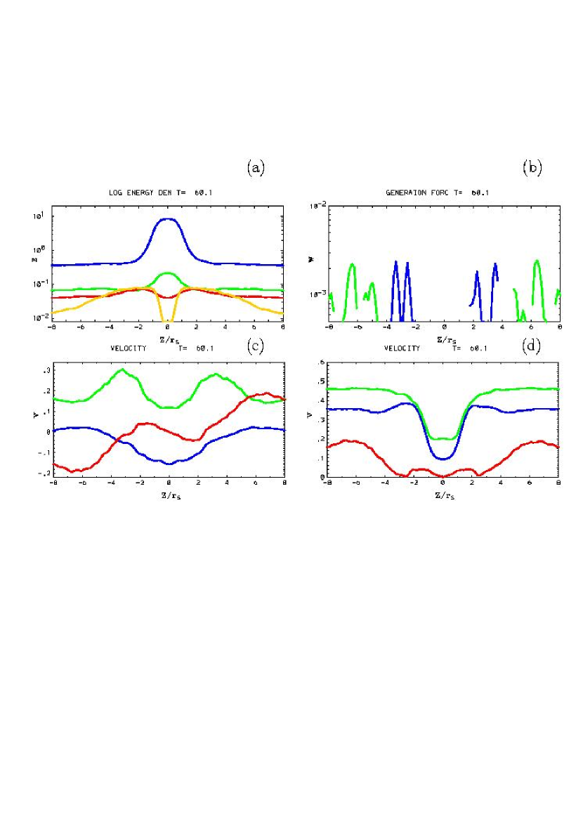
Figure 7: This plot represents various physical quantities on the $x=4.48r_{\rm S}$ surface at $t=60.0\tau_{\rm S}$. Frame (a) shows the values for proper mass density $\rho$ (blue), proper pressure $p$ (green), z component magnetic field energy $B^{2}_{\rm z}/2$ (red), and perpendicular magnetic field energy $B^{2}_{\rm x}+B^{2}_{\rm y}$ (yellow). Frame (b) is the power contribution of the pressure, $W_{\rm gp}$ (green) and the electromagnetic force, $W_{\rm EM}$ (blue). Frame (c) shows the components of the velocity $v_{\rm y}$ (green), $v_{\rm z}$ (red), and $v_{\rm x}$ (blue). Frame (d) shows the Alfvén velocity $v_{\rm A}$ (blue), the sound velocity $v_{\rm S}$ (green), and the velocity $|v_{\rm z}|$ (red).

In order to analyze the properties of jet formation in this simulation, we present the physical variables using several one-dimensional slices along the radial axis and the jet formation axis. Figures 1c and 2c show the density and pressure at time $60.0\tau_{\rm S}$ corresponding to the time of our one-dimensional slices shown in Figs. 5 - 7. At this time the generated jet has maximum velocity. The parameters for these slices where chosen in order to perform comparisons with Koide, Shibata, & Kudoh (1999), and are plotted showing one dimensional radial ($x$-axis) slices along $z=0$, $z=5.6r_{\rm S}$ and $x=4.48r_{\rm S}$ in the Cartesian coordinate (for all figures at $y=0$).

The parameters along the $x$-axis (at $y=z=0$) with the event horizon at $x/r_{\rm S}=\pm 1.0$ are shown in Figure 5. The central gaps in these panels correspond to the black hole region. Figure 5a which shows the density (blue), pressure (green) and $z$-component magnetic field energy $B^{2}_{\rm z}/2$ (red) reveals a shock around $x=\pm 3.0r_{\rm S}$ outside the centrifugal barrier at $x=\pm 2.0r_{\rm S}$. Shock and adiabatic heating due to strong deceleration of the flow yields a relativistic region within $x=\pm 2.0r_{\rm S}$ where $p\approx\rho c^{2}$. Figure 5b shows the power contributions from the gas pressure (green) and electromagnetic field (blue) components independently as depicted in Equations 11 & 12. These energies contribute to decelerating the accretion disk plasma (attention must be given to the sign ($-W$)). The electromagnetic force is produced by the magnetic tension caused by the strongly pinched magnetic field lines as shown in Fig. 4c. The individual magnetic field components are shown in Fig. 5c. The $z$-component $B_{\rm z}$ (red) is pinched by the falling corona and accretion disk. However, other components ($B_{\rm x}$ (blue) and $B_{\rm y}$ (green)) are close to zero. Slight humps in $B_{\rm x}$ (blue) at $x=\pm 2r_{\rm S}$ are found near the black hole but further investigation is necessary to ascertain the cause. The three-velocity components $v_{\rm x}$ (blue), $v_{\rm y}$ (green), and $v_{\rm z}$ (red) are plotted in Fig. 5d. The value of $v_{\rm y}$ reverses at the location of the centrifugal barrier at $x=\pm 2r_{\rm S}$. The inner edge of the disk enters into the unstable orbit region, $|x|\leq 3r_{\rm S}$, as shown in Fig. 5d. The material accretes to the points around $x=\pm 2r_{\rm S}$ but is slowed down by the compressed magnetic field ($B_{\rm z}$ (red)) as seen in Fig. 5c. The advection flow in the unstable orbit region stops at $x\approx\pm 2r_{\rm S}$, and the plasma is ejected in the $z$-direction as shown in Figs. 1c and 2c. Inside the barrier, the plasma is accelerated rapidly to a relativistic velocity near the horizon as seen in Fig. 5d ($v_{\rm x}$ (blue)). This highly heated, high density region should contributes to radiation which can be observed by present and planned space based observatories (see Fabian et al. 2000; Reynolds and Nowak 2003).

Figure 6 shows the same parameters as in Figure 5, but along the $z=5.6r_{\rm S}$ slice ($y=0$). Since this slice is well above the Schwarzschild radius of the black hole, there is not a central gap in the figures. Figure 6b clearly shows the separate layers of the jet resulting from the gas pressure (green around $x=\pm 4r_{\rm S}$) and the electromagnetic forces (blue around $x=\pm 5r_{\rm S}$). A double-layered jet is found where the inner part of the jet is a gas-pressure-driven jet and the outer one is a magnetically driven jet (Koide, Shibata, & Kudoh 1999). From the velocity profiles in Figure 6d, the jet appears to have a width from $3r_{\rm S}\leq|x|\leq 5r_{\rm S}$. The electromagnetically driven component has the larger magnetic field $B_{\rm y},B_{\rm z}$ and a large azimuthal velocity $v_{\rm y}$. It should be noted that at this time ($\tau_{\rm S}=60.0$) a torsional Alfvén wave is excited (Koide, Shibata, & Kudoh 1999). Later the outwards propagation of the TAW contributes to formation of a wind, and as will be discussed later, the peak of $v_{\rm z}$ will move outward.

Figure 7 presents the physical variables along the $x=4.48r_{\rm S}$ slice ($y=0$). This slice is along the vertical axis of the jet rather than the horizontal plane of the disk as in the previous figures (Figs. 5 and 6). The density (blue) and pressure (green) increases are expected around the accretion disk in Fig. 7a. The equatorial plane is located at $z=0$ and the density in the disk is much higher than other values as shown in Fig. 7a. Figure 7b shows the contribution to jet generation due to the electromagnetic field ($2<|z/r_{\rm S}|<4$) (outer part) and gas pressure ($5<|z/r_{\rm S}|<8$) (inner part), and is consistent with the increase of the jet $v_{\rm z}$ (red) in Fig. 7c. However, the region of acceleration due to gas pressure is smaller than in the axisymmetric case. This may come from the fact that the time here is somewhat later than the $t=52\tau_{\rm S}$ in the axisymmetric case and/or due to 3-D effects. The three-velocity components are plotted in Fig. 7c. It should be noted that the jet has a larger azimuthal component ($v_{\rm y}$) near the disk than the $z$ component ($v_{\rm z}$) which becomes larger far from the disk. A slightly positive radial velocity $v_{\rm x}$ (blue) is found far from the disk in Fig. 7c, and this indicates outward angular momentum transfer. The Alfvén velocity $v_{\rm A}$ and the sound velocity $v_{\rm s}$ are shown along with the absolute value of $v_{\rm z}$ in Fig. 7d. The velocity $v_{\rm z}$ gradually increases in the magnetically driven region $5r_{\rm S}\leq z\leq 7r_{\rm S}$ but does not exceed either the sound or Alfvén velocities.

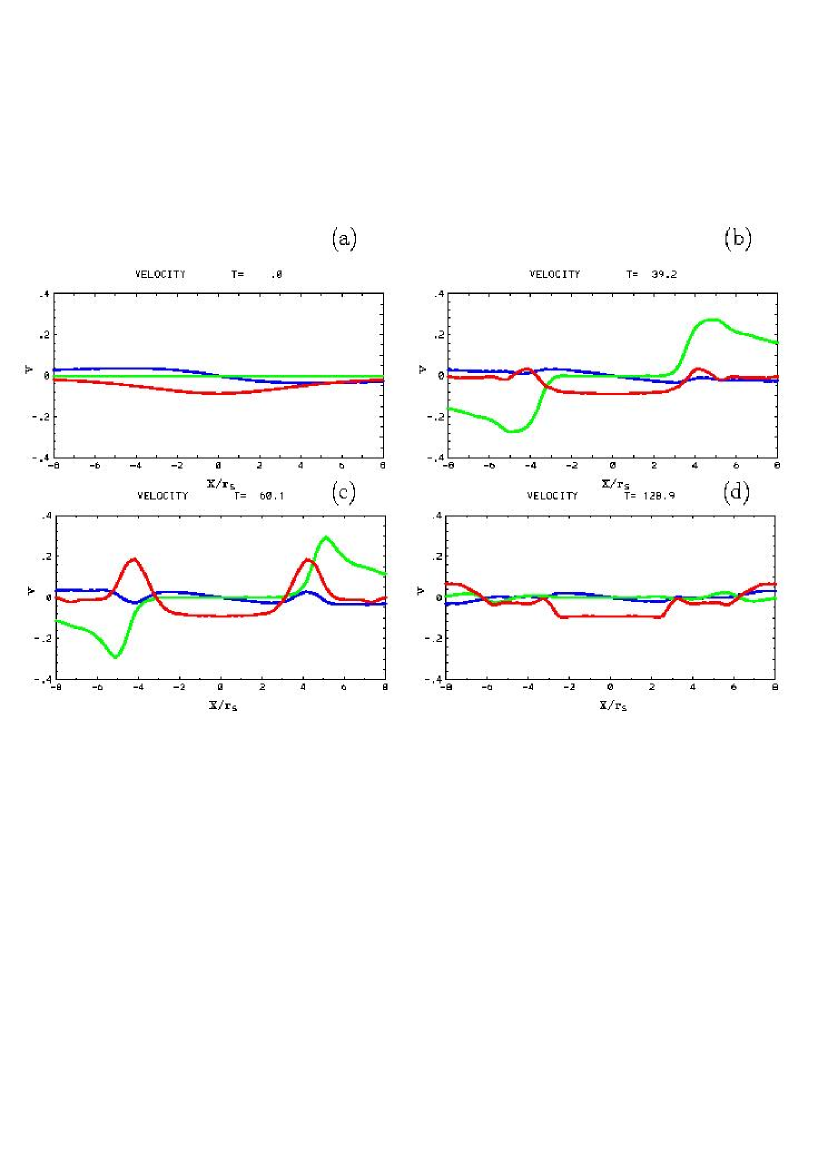
Figure 8: The time evolution of one dimensional slice of velocities through the simulation domain at $z=5.6r_{\rm S}$ is plotted at (a) $t=0.0\tau_{\rm S}$, (b) $t=39.2\tau_{\rm S}$, (c) $t=60.0\tau_{\rm S}$, and (d) $t=128.9\tau_{\rm S}$. The blue, green, and red curves present $v_{\rm x},v_{\rm y}$, and $v_{\rm z}$, respectively.

Figure 8 shows one dimensional slices of the velocities $v_{\rm x}$ (blue), $v_{\rm y}$ (green), and $v_{\rm z}$ (red), at $z=5.6r_{\rm S}$ ($y=0$) for times (a) $t=0.0\tau_{\rm S}$, (b) $t=39.2\tau_{\rm S}$, (c) $t=60.0\tau_{\rm S}$, and (d) $t=128.9\tau_{\rm S}$. The jet is seen in $v_{\rm z}$ (red curve) and its maximum velocity can be found in Fig. 8c. Comparison between the velocity structure at $t=$ $60\tau_{\rm S}$ (Fig. 8c) and $80\tau_{\rm S}$ (not shown) reveals that the jet velocity ($v_{\rm z}$) and the azimuthal velocity ($v_{\rm y}$) are smaller at $t=80\tau_{\rm S}$. Additionally, the location of peak velocities ($v_{\rm z}$) are shifted outward at the later time. This may come from the fact that the wind is caused by the unwinding magnetic fields with the TAWs which are propagating outward in the disk. These results are consistent with the fact that the jet has faded and a weak wind is generated around $x=7r_{\rm S}$ as seen in Fig. 8d. Furthermore, the rotation of the accretion disk ($v_{\rm y}$) becomes very small and rotates slightly in the reverse direction around $x=\pm 3.5r_{\rm S},$ and $\pm 7r_{\rm S}$. We plan to investigate how these changes are affected by inflow of matter to the system in the future.

A comparison of our present results with previous two-dimensional results shown in Koide, Shibata, & Kudoh (1999) reveals some minor differences that may be due to the three-dimensional modeling. The most prominent difference between this 3-D simulation and previous 2-D simulations lies in the longer run time and hence shows a significant change in the disk-jet system to a disk-wind system (Fender 2002, 2003). This transition may be caused by outward TAW propagation in the disk. The jet is mainly produced by the gradient of gas pressure enhanced by the shock around $r=3r_{\rm S}$, as shown in Figs. 1c, 3c and 6b. After $t=60\tau_{\rm S}$, the TAW moves outward in the disk and is weakened. The wind appears while the TAW is moving outward. After outward propagation of the TAW, the pressure of the outer disk becomes larger than the initial condition (Fig. 2a). Therefore, the wind may be caused by unwinding of the twisted and pinched magnetic fields due to the decreased accreting matter, which creates the TAW propagating outward in the disk. This transient change may be controlled by the mass accretion rate onto the black hole. It should be noted that in the simulations with initial weak azimuthal magnetic fields the magnetic fields are tangled as shown in Fig. 6 in Hirose et al. (2004) as a result of MRI where TAWs are not excited.

5 Summary and Discussion

We have presented a fully 3-D GRMHD simulation of a Schwarzschild black hole accretion disk system with moderate resolution. Because no deliberate asymmetric perturbation was introduced, the present 3D simulation remains largely axisymmetric. While we found some numerical differences between this simulation and previous two-dimensional simulations, our results reaffirm the previous result of a two-layered jet. Our results suggest that the jet develops as in the 2-D case. Our longer simulation has allowed us to study jet evolution. At the end of this simulation the jet fades and a weak wind is generated by a thickened accretion disk. This phenomena was not observed in the two-dimensional simulations because they did not run for this duration.

In this simulation at the outer boundary of the accretion disk no matter is injected, therefore after accreted matter is ejected from the accretion as a jet, the power to generate a jet is dissipated and the jet is switched to a wind. However, if streaming matter is injected at the outer boundary of accretion disk, transient changes may be controlled by accretion rates with instabilities and be related to the state transitions. Such disk-jet coupling in black hole binaries is reviewed by Fender (2002, 2003) and Fender, Belloni, & Gallo (2004). Black hole binaries exhibit several different kinds of X-ray ‘state’. The two most diametrically opposed, which illustrate the relation of jet formation to accretion, can be classified as low/hard/off and high/soft states (Fender 2003). These two states provide different luminosity. Pellegrini et al. (2003) have discussed a nuclear bolometric luminosity and an accretion luminosity $L_{\rm acc}$ in terms of the accretion rate $\dot{M}$ and jet power. Clearly these issues can be investigated by further 3-D GRMHD simulations, and future simulations will investigate jet formation with different states of the black hole including streaming material from an accompanying star (e.g., Miller et al. 2003).

Additionally, we plan to study the development of instabilities along the azimuthal direction such as the proposed accretion-ejection instability (AEI) (e.g. Tagger & Pellat 1999; Caunt & Tagger 2001; Rodriguez et al. 2002; Vaniére, Rodriguez & Tagger 2002), the magnetorotational instability (MRI) (e.g. Balbus & Hawley 1991, 1998), and the “screw” (current-driven helical kink) instability (e.g. Li 2000). Such simulation studies may indicate how the observed variabilities in AGN jets (Blandford 2003; Mirabel 2003) and microquasars (e.g. Eikenberry et al. 1998; Ueda et al. 2002; Nobil 2003; Rau, Greiner, & McCollough 2003) can be produced. Initial magnetic field configurations affect the dynamics of accretion disks and the associated phenomena such as jet formation and its variabilities, and thus we plan to study different initial field configurations.

The Fe K$\alpha$ fluorescent emission line in active galactic nuclei (AGN) is believed to originate in a relativistic accretion disk around a black hole (e.g. see reviews Fabian et al. 2000; Reynolds & Nowak 2003). The X-ray continuum emission of MCG-6-30-15 is highly variable (e.g. Vaughan & Fabian 2003). The source spectrum and variablity can be explained by two-components consisting of a variable power law component (PLC) and an almost constant reflection-dominated component (RDC) containing the iron line (Fabian & Vaughan 2003). The region where the flare (or multiple flares) which created the PLC must be located close to the rotation axis and within 3-4 gravitational radii to reproduce the highly variable behavior, (Miniutti et al. 2003). Since this behavior is most likely powered by magnetic field from the disk, possibly linking to the hole (e.g. Blandford & Znajek 1977; Wilms et al. 2001), and perhaps forming the base of jet, it is essential to perform GRMHD simulations. These issues are being investigated with 3-D GRMHD simulations with a Kerr black hole with streaming matter from an accompanying star.

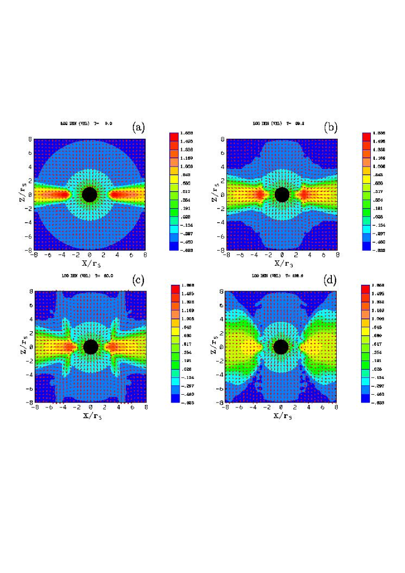
Figure 1: The panels present the time evolution of the proper mass density (color) with velocity arrows ($v_{x},v_{z}$) in a transonic free-fall (steady-state falling) corona with an initially uniform magnetic field, at (a) $t=0.0\tau_{\rm S}$, (b) $t=39.2\tau_{\rm S}$, (c) $t=60.0\tau_{\rm S}$, and (d) $t=128.9\tau_{\rm S}$. The black hole’s Schwarzschild radius is presented by the central black circle in each panel. The jet is fully formed at $t=60.0\tau_{\rm S}$ (c). At the later time the wind is formed with a wider angle.

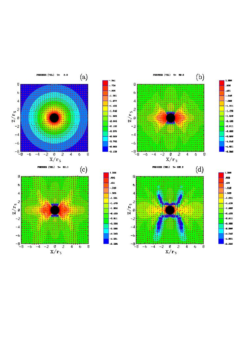
Figure 2: These panels present the time evolution of the proper pressure (color) with velocity arrows ($v_{x},v_{z}$) in a transonic free-fall (steady-state falling) corona with an initially uniform magnetic field, at (a) $t=0.0\tau_{\rm S}$, (b) $t=39.2\tau_{\rm S}$, (c) $t=60.0\tau_{\rm S}$, and (d) $t=128.9\tau_{\rm S}$.

References

- Armitage, Reynolds, & Chiang (2001) Armitage, P. J., Reynolds, C. S., & Chiang, J. 2001, ApJ, 548, 868
- Balbus & Hawley (1991) Balbus, S. A. & Hawley, J. F. 1991, ApJ, 376, 214
- Balbus & Hawley (1998) Balbus, S. A. & Hawley, J. F. 1998, Rev. Mod. Phys., 70, 1
- Blandford (2002) Blandford, R. D. 2002, Lighthouses of the Universe, ed. M. Gilfanov, R. Sunyaev et al. Berlin:Springer. 206
- Blandford (2003) Blandford, R. D. 2003, Active Galactic Nuclei: from Central Engine to Host Galaxy, ed. S. Collin, F. Combes and I. Shlosman. ASP (Astronomical Society of the Pacific), Conference Series, Vol. 290, p. 267
- Blandford & Payne (1982) Blandford, R. D., & Payne, D. G. 1982, MNRAS, 199, 883
- Blandford & Znajek (1977) Blandford, R. D., & Znajek, R. 1977, MNRAS, 179, 433
- Bondi (1952) Bondi, H. 1952, MNRAS, 112, 195
- Bondi & Hoyle (1944) Bondi, H. & Hoyle, F. 1944, MNRAS, 104, 273
- Caunt & Tagger (2001) Caunt, S. E. & Tagger, M. 2001, A&A, 367, 1095
- Davis (1984) Davis, S. F., 1984 NASA Contractor Rep. 172373, ICASE Rep., No. 84-20.
- De Villiers & Hawley (2002) De Villiers, J. P., & Hawley, J. F. 2002, ApJ, 577, 866
- De Villiers & Hawley (2003a) De Villiers, J. P., & Hawley, J. F. 2003a, ApJ, 589, 458
- De Villiers & Hawley (2003b) De Villiers, J. P., & Hawley, J. F. 2003b, ApJ, 592, 1060
- De Villiers, Hawley, & Krolik (2003) De Villiers, J. P., Hawley, J. F. & Krolik, J. H. 2003, ApJ, 599, 1238
- De Villiers, Hawley, Krolik, & Hirose (2004) De Villiers, J. P., Hawley, J. F. & Krolik, J. H. 2004, ApJ, in press, (astro-ph/0407092)
- Eikenberry et al. (1998) Eikenberry, S. S., Matthews, K., Morgan, E. H., Remillard, R. A., & Nelson, R. W. 1998, ApJ, 494, 61L
- Fabian & Vaughan (2003) Fabian, A. C., & Vaughan, S. 2003, MNRAS, 340, L28
- Fabian et al. (2000) Fabian, A. C., Iwasawa, K., Reynolds, C. S., Young, A. J. 2000, PASP, 112, 1145
- Ferrari (1998) Ferrari, A. 1998, ARAA, 36, 539
- Fender, Belloni, & Gallo (2004) Fender, R., Belloni, T. M., & Gallo, E. 2004, MNRAS, submitted (astro-ph/0409360)
- Fender et al. (2004) Fender, R., Wu, K., Johnston, H., Tzioumis, T., Jonker, P., Spencer, R., & van der Klis, M., 2004, Nature, 427, 222
- Fender (2002) Fender, R. 2002, Relativistic flows in Astrophysics, Springer Verlag Lecture Notes in Physics, Ed. A.W. Guthmann, M. Georganopoulos, K. Manolakou and A. Marcowith, v. 589, 101
- Fender (2003) Fender, R. 2003, in Compact Stellar X-Ray Sources’, ed. W.H.G. Lewin & M. van der Klis, Cambridge University Press
- Gammie, McKinney, & Tóth (2003) Gammie, C. F., McKinney, J. C., & Tóth, G. 2003, ApJ, 589, 444
- Hawley (2000) Hawley, J. F., 2000, ApJ, 528, 462
- Hawley (2001) Hawley, J. F., 2001, ApJ, 554, 538
- Hawley & Balbus (2002) Hawley, J. F., & Balbus, S. A. 2002, ApJ, 573, 738
- Hawley, Balbus, & Stone (2001) Hawley, J. F., Balbus, S. A., & Stone J. M. 2001, ApJ, 554, L49
- Hawley & Krolik (2001) Hawley, J. F. & Krolik, J. H., 2001, ApJ, 548, 348
- Hawley & Krolik (2002) Hawley, J. F. & Krolik, J. H., 2002, ApJ, 566, 164
- Hirose et al. (2004) Hirose, S., Krolik, J., De Villiers, J. P., & Hawley, J. F. 2004, ApJ, 606, 1083
- Igumenshchev, Abramowicz, & Narayan (2000) Igumenshchev, I. V., Abramowicz, M. A., & Narayan, R. 2000, ApJ, 537, L27
- Igumenshchev, Narayan, & Abramowicz (2003) Igumenshchev, I. V., Narayan, R., & Abramowicz, M. A. 2003, ApJ, 592, 1042
- Koide (2003) Koide, S. 2003, Phys. Rev. D, 67, 104010
- Koide et al. (1996) Koide, S., Nishikawa, K.-I., Mutel, R. L. 1996, ApJ, 463, L71.