WMAP constraints on inflationary models with global defects

Abstract

We use the cosmic microwave background angular power spectra to place upper limits on the degree to which global defects may have aided cosmic structure formation. We explore this under the inflationary paradigm, but with the addition of textures resulting from the breaking of a global $O(4)$ symmetry during the early stages of the Universe. As a measure of their contribution, we use the fraction of the temperature power spectrum that is attributed to the defects at a multipole of 10. However, we find a parameter degeneracy enabling a fit to the first-year WMAP data to be made even with a significant defect fraction. This degeneracy involves the baryon fraction and the Hubble constant, plus the normalization and tilt of the primordial power spectrum. Hence, constraints on these cosmological parameters are weakened. Combining the WMAP data with a constraint on the physical baryon fraction from big bang nucleosynthesis calculations and high-redshift deuterium abundance limits the extent of the degeneracy and gives an upper bound on the defect fraction of 0.13 (95% confidence).

I Introduction

Recent measurements of the cosmic microwave background (CMB), notably the first year WMAP data Hinshaw et al. (2003); Kogut et al. (2003), have proved highly successful in probing the early stages of cosmic structure formation. The observed CMB anisotropies may be produced by taking adiabatic primordial perturbations of roughly the Harrison-Zel’dovich form and evolving these using well-understood, linear physics. Further, the parameter values that are required for this process to a give a match to the data are consistent with those measured using other astronomical techniques. That the primordial power spectrum predicted by many models of inflation is of the required form has become an important success of the inflationary paradigm.

On the other hand, a less attractive property of the paradigm is that successful inflationary models may involve quite different fields, interactions and levels of physical motivation. Here we address the issue using CMB power spectra to constrain models of hybrid inflation Linde (1994); Lyth and Riotto (1999) that involve the formation of topological defects as inflation ends Copeland et al. (1994). Such models, however, do not fit exactly into the above regime. With the existence of topological defects, the seeding of cosmic structure continues after inflation ends, for the defects further perturb the cosmic fluid as long as they continue to be present. For a detailed review of structure formation with defects see Ref. Durrer et al. (2002), but generally, a defect-dominated temperature power spectrum does not have pronounced acoustic peaks Albrecht et al. (1996). Hence, if defects are added to a passive-evolution case and the normalization reduced to maintain the fit to data on large scales, then the acoustic peaks are slightly suppressed. That is, however, assuming that the other cosmological parameters are not also changed.

Earlier work along these lines Battye and Weller (2000); Bouchet et al. (2001); Contaldi et al. (1999); Jeannerot (1997); Pogosian et al. (2003) has tended to be of quite a different vein to that described here. In particular we employ a full likelihood analysis for the fit to data in which the cosmological parameters are free to vary. This freedom has important consequences for the independent use of the temperature power spectrum to constrain such hybrid models — at least given the presently available data. Previous studies have also tended to focus on local defects in the form of cosmic strings, a class of models that we shall not look at here in any detail, and of such work only Pogosian et al. (2003) has involved data from the WMAP project.

In our work, the cosmological perturbations are the uncorrelated sum of those from (i) an inflationary adiabatic model, including both scalar and tensor perturbations, and (ii) a global defect model, with an $O(4)$ symmetry breaking at (or after) the end of inflation producing textures (see e.g. Durrer et al. (2002)). In parametrizing the primordial perturbations, we take there to be negligible running of the scalar spectral index and that the tensor index obeys the single-field consistency condition (see Sec. III). We also assume negligible neutrino masses, as would result from a hierarchical mass variation with neutrino flavor.

The contribution to the CMB power spectra from inflation is found using a variant of the CMBFAST Seljak and Zaldarriaga (1996) approach, in the form of CAMB Lewis et al. (2000). The defect contribution is found by applying the unequal-time correlator (UETC) approach Pen et al. (1997) to numerical field evolution simulations, as will be discussed in the next section. The UETC method addresses the problem that, in order to calculate CMB power spectra to sub-degree scales, a simulation conventionally requires a dynamic range that is far in excess of that which is feasible with current technology. While it is possible to make full-sky CMB maps Pen et al. (1994); Landriau and Shellard (2004), this direct approach is currently limited to relatively low multipoles: $\ell<20$, although these potentially contain more information than the power spectra alone. The UETC method boosts the dynamic range via a series of theoretical simplifications, for example causality, such that high resolution power spectra calculations may be performed from the simulation data. To do so also involves calculations of the CMBFAST-type, which we carried out using a version of CMBEASY Doran (2003) modified so as to deal with the defect scenario.

Despite the benefits of the UETC approach, the computational requirements of CMB calculations that include defects far exceed those that do not. As a result, the calculation of CMB spectra for a vast number of different cosmological parameter values is not attainable. Hence, the popular Markov chain Monte Carlo (MCMC) approach Verde et al. (2003); Lewis and Bridle (2002); Gelman and Rubin (1992), which involves many thousand such calculations, cannot be fully applied to the defect case. However, the non-defect case fits the WMAP data well and defect-dominated structure formation does not give the required acoustic peaks, suggesting that the defect contribution is small. If this is the case, then the result of a small change in the cosmological parameters used for the defect calculation is a second order effect. Therefore, the defect contribution needs only to be calculated once, using currently favored values of the cosmological parameters (see Sec. II). The defect contribution is then fixed, except for a normalization factor, which is free since it is not known at which energy scale the defects formed. Hence the approach used here, which is described more fully in Sec. III, is to apply the standard MCMC procedure to the primordial contribution and add in the defect component with its normalization varied as an MCMC parameter. This has been achieved using a slightly modified version of CosmoMC Lewis and Bridle (2002), which is directly linked to CAMB. As this extra parameter controls the degree to which the CMB power spectra differ from the usual non-defect spectra, it shall be the main focus of this paper.

However, we shall not present our results in terms of this parameter directly. Rather we shall use the fractional defect contribution to the temperature power spectrum at a particular multipole, $\ell=10$. The correspondence between the two is roughly linear for low fractions but with a slight spread due to the variation of the non-defect contribution to the chosen multipole. The fractional quantity is, however, more directly understandable.

The data that we have used here are principally that from the first year WMAP release Hinshaw et al. (2003); Kogut et al. (2003): the temperature power spectrum and the temperature-polarization (TE) cross-correlation spectrum. Other CMB projects, such as ACBAR Kuo et al. (2004), CBI Pearson et al. (2003); Readhead et al. (2004) and VSA Dickinson et al. (to be published), which give data out to higher multipoles than WMAP do not provide much in the way of additional constraints on our model. Applying data on cosmological parameters from, for example, work on big bang nucleosynthesis (BBN) Kirkman et al. (2003) and measurements of the Hubble parameter by the Hubble Key Project (HKP) Freedman et al. (2001) has proved more important, as will be detailed in section III.

The changes to the matter power spectrum that the inclusion of defects causes may be found in an entirely analogous manner to the CMB calculation. However, while there have been recent steps forward in measurements of this from galaxy redshift surveys, such as 2DFGRS Percival et al. (2001) or SDSS Tegmark et al. (2003), and from the Lyman-$\alpha$ forest Croft et al. (2002), we have chosen not to use such data. Galaxy formation in the presence of defect-induced density perturbations is not understood, and even in pure inflation scenarios, inferences from the Lyman-$\alpha$ forest must be drawn with care Seljak et al. (2003). Further, we do not believe that the use of such data would significantly change our results, as we shall discuss in Sec. III. This is a conservative position, driven by our desire to make reliable and statistically meaningful statements about the relative importance of global defects.

II CMB calculations in global topological defect models

The procedure to obtain the defect power spectra contribution for both the CMB and for dark matter is as in Durrer, Kunz and Melchiorri Durrer et al. (2002) and is fully detailed there. The method consists of two distinct steps, the first of which is to compute the unequal time two-point correlation functions $C_{\mu\nu\rho\lambda}$ of the defect energy momentum tensor $T_{\mu\nu}$:

$$C_{\mu\nu\rho\lambda}(k,t,t^{\prime})=\left\langle T_{\mu\nu}(k,t)T_{\rho\lambda}^{*}(k,t^{\prime})\right\rangle.$$ (1)

This is done with a numerical simulation of the classical $O(4)$ non-linear sigma model on a three-dimensional grid. For global defects, where the seed energy momentum tensor can be taken to be separately conserved, only five UETCs are independent, three for the scalar perturbations and one each for the vector and tensor perturbations. As topological defects generate perturbations at all times after their creation, the vector perturbations do not decay and have to be taken into account. Also, the relative amplitudes are fixed by the model and cannot be adjusted.

However, as already mentioned, the overall normalization of the perturbations is related to be symmetry-breaking scale $\eta$ and is free to be varied. Roughly, the relation to the CMB temperature anisotropy $\delta T$ is as

$$\frac{\delta T}{T}\sim\Psi\sim 4\pi G\eta^{2},$$ (2)

where $\Psi$ is the dimensionless gravitational potential and $G$ is Newton’s constant. Hence, the dependence of $\eta$ upon the the normalization of power spectrum $A_{\rm d}^{2}$ (with the square highlighting that the spectrum is quadratic in the perturbations) is

$$\eta\sim(A_{\rm d}^{2})^{\frac{1}{4}}.$$ (3)

Therefore $A_{\rm d}^{2}$ is not a sensitive measure of $\eta$. In fact, the constraints upon $\eta$ from references herein are not likely to be greatly changed by our results. Hence, here we focus solely upon the significance of the defect perturbations compared to those of primordial origin.

For this work, we used the simulations made for Durrer et al. (1999), which used a $256^{3}$ grid. The results agree well with analytic predictions Durrer and Kunz (1998) and the simulations of Pen et al. (1997). The UETCs were computed separately for radiation and matter dominated backgrounds. In a background dominated by a cosmological constant, the defects are quickly inflated away, so that their contribution to the total energy-momentum tensor decays rapidly and can be neglected.

The UETCs then act in the second step as external sources for a Boltzmann solver. These codes need a deterministic source $S(k,t)$, but the defects are essentially random by nature. We circumvent this problem by diagonalizing each UETC, which through discretization and the assumption of scaling evolution can be represented by a matrix with indices $kt$ and $kt^{\prime}$. This is hence a means of writing the full, incoherent source as the sum of coherent sources $v_{n}$ Turok (1996):

$$C(kt,kt^{\prime})=\sum_{n}\lambda_{n}v_{n}(kt)v_{n}^{*}(kt^{\prime}).$$ (4)

To this end, we discretized the correlation functions into matrices of size $200\times 200$, which can then be diagonalized with the help of standard methods. On a somewhat technical aside, the three scalar UETCs are combined into one $400\times 400$ matrix and diagonalized together, as the third matrix represents the correlation (off-diagonal part) between the other two. The discretization can be performed in different ways, e.g. by taking linear or logarithmic intervals in $kt$. We use linear intervals as we found that this improves the convergence of the results (but more care must be taken in this case to ensure that the dynamical range is sufficient).

We interpolate the resulting eigenvectors $v_{n}(kt)$ with cubic splines and use them as the sources for the Boltzmann solver. The power spectra are then given by

$$C_{\ell}=\sum_{n}\lambda_{n}^{(S)}C_{\ell}^{(S)n}+\sum_{n}\lambda_{n}^{(V)}C_{\ell}^{(V)n}+\sum_{n}\lambda_{n}^{(T)}C_{\ell}^{(T)n},$$ (5)

and correspondingly for the dark matter power spectrum $P(k)$. We use the $20$ eigenvectors with the largest eigenvalues, which is more than sufficient as the last ones contribute far less than 1%.

Linear cosmological perturbation theory with seeds has been discussed extensively in the literature. We work in the gauge-invariant formalism of Durrer et al. (2002) with a modified version of the CMBEASY Boltzmann code, using the total angular momentum method Hu and White (1997). The sources are interpolated between matter and radiation dominated epochs, and are gradually suppressed as the cosmological constant starts to dominate.

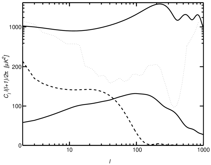
Figure 1: The temperature power spectrum contributions from the global defects compared to that from primordial tensor perturbations and to the more dominant primordial scalar contribution. The defect and tensors contributions are scaled such that their contributions at $\ell=10$ are 13% and 19% respectively of a scalar-only fit to the WMAP data. (Note that the ordinate axis has linear scaling below $300\>\mu\rm K^{2}$ but logarithmic scaling above this value so as to show the slowly-varying defect contribution well on the same plot as the scalar contribution.) The dotted line indicates the 2$\sigma$ uncertainty in the WMAP data, including cosmic variance.

The fixed form of the defect contribution to the temperature power spectrum for this case is illustrated in Fig. 1 (and was calculated using flat geometry, $h=0.70$, $\Omega_{\rm b}h^{2}=0.022$, $\Omega_{\rm m}=0.30$ and $\tau=0.10$ or $z_{\rm r}=13$ — see Sec. III for definitions). The figure compares it with the primordial scalar contribution (shown on a log scale) and that resulting from primordial tensor perturbations. The defect spectrum is scaled so as to match our final result for the 95% upper bound on the fractional contribution (see section III). The corresponding contribution to the TE cross-correlation spectrum is very small and hence while it is incorporated in our calculations we shall not illustrate it here (however, see Seljak et al. (1997) for a plot).

We expect that the overall error in the defect calculation is smaller than about 10%, and checked that our power spectra agree with other published results Pen et al. (1997); Durrer et al. (2002) to within this accuracy. Comparing the fixed defect spectrum used with a second one, calculated using a different cosmology ($h=0.80$, $\Omega_{\rm b}h^{2}=0.027$), shows that the changes in the defect contribution are smaller than about 10% over the WMAP data range. For the case illustrated in Fig. 1, the defect contribution to the temperature power spectrum is of the same order as the uncertainties from measurement plus cosmic variance, in which case, such errors in our approach are not significant for the comparison to data.

The final step is to simply add the defect contribution, with the appropriate normalization, to that resulting from the primordial scalar and tensor perturbations. This is justified by the fact that the quantum fluctuations in the inflaton field and the symmetry breaking field are uncorrelated during inflation when the global symmetry is unbroken. Any subsequent interaction will be second order in the gravitational perturbation and will hence be negligible.

III Monte Carlo parameter fitting

III.1 MCMC overview

The MCMC approach has found recent application to CMB work principally because it allows inferences to be made about the $n$ parameters in a model without requiring a complete and detailed knowledge of the $n$-dimensional likelihood surface. For example, to calculate the likelihood surface on an $n$-dimensional grid consisting of $m$ points in each dimension requires $m^{n}$ iterations. In the case of a four parameter model, calculating 50 points in each direction requires $6\times 10^{6}$ iterations. Suppose that each iteration involves the calculation of the CMB power spectra from primordial perturbations for comparison to WMAP data. This amounts to $3\>\rm s$ per iteration using CAMB on a single processor of the UK National Cosmology Supercomputer and around 6 months in total. However, the MCMC approach allows a reliable knowledge of the one-dimensional likelihood function for each parameter (with all the other parameters integrated out) in less than perhaps 100 000. This corresponds to a few days of calculation and this is not sensitively changed by the addition of extra parameters. Higher dimensional functions may be found, in order to plot say a 95% confidence contours of parameter pairs, but the resolution is dependent upon the number of iterations.

The MCMC method incorporated in CosmoMC is the Metropolis-Hastings algorithm. This is a random walk through parameter space, with the parameters recorded at each step to form a Markov chain. Each iteration involves first the generation of a proposed next point in the chain, found by generating a random change in one or more parameters based upon some probability distribution. The form of the distribution is not important for the end result, as long as the probability of proposing point B from point A is the same as proposing point A from point B. The power spectra are calculated for the corresponding parameter set and then the likelihood of these spectra is found from the data. If the likelihood at the proposed point is greater than at the old point, then it is accepted and forms the next point in the chain. Otherwise, a uniformly distributed random number is generated between zero and unity and the proposed point is accepted only if this number is greater than the ratio of the new to old likelihoods. If the proposal is rejected, then the original point is repeated in the chain.

In the limit of infinite such iterations, the number of points in particular volume of parameter space is proportional to the probability of the true parameters lying in that volume. This has a number of attractive properties, for example, the mean value of parameter in a chain is the expectation value of that parameter given the data. Furthermore, the marginalized likelihood function for a parameter is represented simply by a histogram of the values from the chain.

Of course, an infinite chain is not attainable (our chains have lengths of a few hundred thousand elements) and this presents a number of problems. First, the chain is started from some arbitrary location and the first thousand or so points may be highly dependent upon this and carry a finite weighting in the chain. The usual solution is to discard the beginning of the chain and we have followed Gelman and Rubin Gelman and Rubin (1992) in removing the entire first half. However, an analysis is still required to check if an inference from the remaining points in the chain is reliable, given that a finite chain may not have explored all of the relevant parameter space to the same extent. The solution is to use $M$ chains (here we use $M=5$), each started from a different point. If the results of all of these chains agree, then confidence is high in any inferences made. To decide if the $M$ chains compare favorably we have again followed the approach of Gelman and Rubin. This is to make to a comparison for each parameter between the spread within each chain and the spread of the means from the chains. See Refs. Gelman and Rubin (1992) and Verde et al. (2003) for a more details on this comparison.

While we have said that the form of the proposal distribution does not affect the final result, it has a large effect on the efficiency of the approach. The taking of very small steps requires a great many of them to be made in order to fully explore the parameter space. On the other hand, taking large steps increases the chance of proposed-point rejections, and the exploration of the parameter space is inefficient. The approach used here uses the covariance matrix, found from a preliminary run, to set the appropriate step scale. Furthermore, the direction of the step in the $n$-dimensional space is determined using the covariance matrix diagonalization approach implemented in CosmoMC, which deals well with linear degeneracies in the parameter space.

III.2 Model parameters

The cosmological parameters that we have chosen to vary are (i) the Hubble constant ($100h\>\rm{km}\>\rm{s}^{-1}\>\rm{Mpc}^{-1}$), (ii) the physical baryon density $\Omega_{\rm b}h^{2}$, (ii) the total matter density $\Omega_{\rm m}h^{2}$ (via the cold dark matter density $\Omega_{\rm c}h^{2}$), and (iv) the optical depth $\tau$ from the surface of decoupling or rather the redshift of quasi-instantaneous re-ionization $z_{\rm r}$. We have assumed that the Universe is flat as appropriate for an inflationary model, and in any case a change in the curvature gives an almost identical effect as a change in $h$, via the geometric degeneracy Efstathiou and Bond (1999). The effect of allowing a small curvature can therefore be created by change in the Hubble parameter. We will, however, consider constraining $h$ later and so the explicit assumption of zero curvature will then be made.

The primordial power spectrum for scalar perturbations, or more precisely the comoving curvature perturbation, has been parametrized by (v) the normalization $A_{\rm s}^{2}$ and (vi) the spectral index $n_{\rm s}$. The normalization is set at a comoving wavevector $k_{0}$ of 0.01 Mpc^-1 and we assume negligible variation of the spectral index with scale. The scalar power spectrum is hence given by

$${\cal P}_{\rm s}=A_{\rm s}^{2}\left(\frac{k}{k_{0}}\right)^{n_{\rm s}-1}.$$ (6)

A finite contribution to the primordial perturbations from gravitational waves has been allowed for. As shown in Fig. 1, the contribution these tensor perturbations make to the temperature spectrum is to raise very large scales only and hence the tilt in this spectrum must be very large to be detectable in this sub-dominant component. If we assume that the effective mass of the field involved in the global symmetry breaking is much greater than the Hubble parameter during inflation, and the hybrid model involves only this field plus the inflaton, then we may use the single-field inflation consistency relation. Following Leach et al. (2002) we use the primordial form of this relation, giving the tensor tilt in terms of the ratio of the primordial tensor and scalar power spectra at the pivot scale $k_{0}$. This assumption is, however, not important given the current data, and hence we are justified in parametrizing primordial tensor perturbation only by (vii) the normalization $A_{\rm t}^{2}$ (via the ratio $A_{\rm t}^{2}/A_{\rm s}^{2}$):

$${\cal P}_{\rm t}=A_{\rm t}^{2}\left(\frac{k}{k_{0}}\right)^{-\frac{1}{8}\frac{A_{\rm t}^{2}}{A_{\rm s}^{2}}}.$$ (7)

The final parameter that we have varied is then (viii) the normalization of the defect contribution to the CMB power spectra $A_{\rm d}^{2}$, giving a total of 8 parameters.

III.3 Degeneracies, additional data and results

As mentioned in the Introduction, we shall not present our results in terms of $A_{\rm d}^{2}$ but in terms of the fractional defect contribution to the temperature power spectrum at $\ell=10$: $f_{\rm d}$ (and likewise for tensors: $f_{\rm t}$). This particular multipole lies in a region where the temperature power spectrum is relatively flat and has become a conventional place to make contribution ratios. However, this value of $\ell$ happens to be roughly where the fractional defect contribution is greatest. The value at the first peak is approximately one tenth of this, a fact that should be taken into account when interpreting our results.

Naively, $f_{\rm d}$ is tightly constrained by the WMAP data because the contribution to the temperature power spectrum is greatest at scales were the data is very precise (see Fig. 1). However, as is often the case in CMB parameter fitting, $f_{\rm d}$ is involved in a degeneracy with four other parameters, such that an increase in its value may be compensated for by changes in the others and a fit to data maintained. This may be understood broadly as follows. The effect that increasing $A_{\rm d}^{2}$ has on the temperature power spectrum is to the raise the region $\ell<400$. This may be reversed by lowering the normalization of the primordial scalar perturbations using $A_{\rm s}^{2}$ and giving a slight tilt toward small scales using $n_{\rm s}$. (Increasing $\tau$ also has the general effect of reducing the temperature anisotropies, although the influence of $\tau$ tails off for $\ell\lesssim 100$ and is hence less important here.) Unfortunately, the temperature power spectrum is most sensitive to the decrease in $A_{\rm s}^{2}$ at the first peak and, as a result, it is excessively lowered. Further tilting the primordial scalar spectrum can raise the first peak but at the expense of raising the high-$\ell$ region too far. However, an increase in $\Omega_{\rm b}h^{2}$ raises the first peak while lowering the region around the second and third peaks and therefore, combined with extra tilt, this achieves the desired effect. The fit may then be further improved, for the increases in both $n_{\rm s}$ and $\Omega_{\rm b}h^{2}$ raise the high $\ell$ side of the first peak more than the low $\ell$ side (outweighing the opposite effect of the defects). This may be countered by using the Hubble constant to move the peak to slightly lower $\ell$ and give an overall result that, considering the data, is almost indistinguishable from the original.

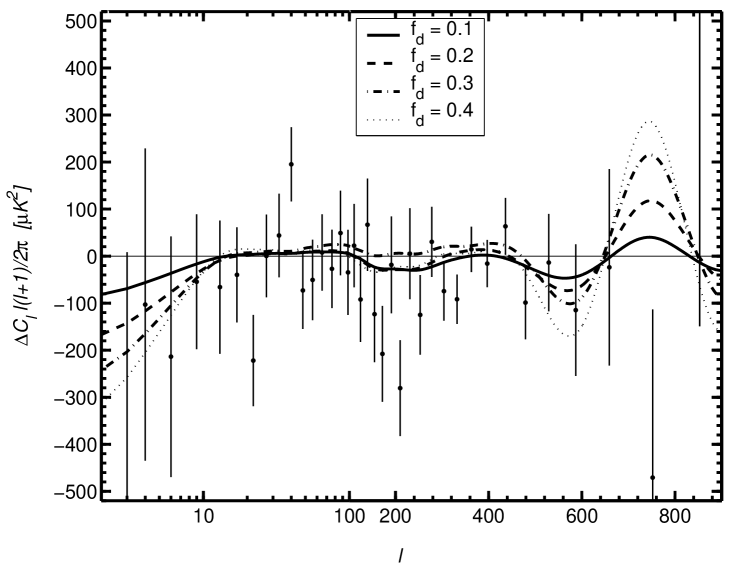
Figure 2: The change in the temperature power spectrum from a model without defects, when defects are added and degeneracy direction followed to maintain the fit to data. The WMAP first-year binned data are over-plotted, with the zero-defect model subtracted from them, demonstrating the inability of the data to readily distinguish between the models. The error bars include cosmic variance. (Note that multipole axis is linear for $\ell>200$ and logarithmic below this in order to show both regions clearly.)

$f_{\rm d}$	$\Omega_{\rm b}h^{2}$	$h$	$10^{10}A_{\rm s}^{2}$	$n_{\rm s}$
0.0	0.026	0.81	24	1.05
0.1	0.028	0.86	22	1.10
0.2	0.031	0.93	21	1.17
0.3	0.034	1.03	19	1.25
0.4	0.039	1.16	17	1.35

Table 1: Parameter values corresponding to the cases considered in Fig. 2 (see Sec. III for definitions). The following parameters are fixed: $\Omega_{\rm m}h^{2}=0.13$, $z_{\rm r}=17$, $f_{\rm t}=0.15$. The others are set as the means found from a sub-set of an MCMC chain, selected such that the defect fraction and these fixed parameters have approximately the correct values.

Figure 2 shows the change in the temperature power spectrum from a non-defect case that is caused by adding in defects at four different levels: $f_{\rm d}=0.1$, $0.2$, $0.3$, $0.4$. The other four parameters of the degeneracy have been adjusted, as shown in Table 1, so that the fit is maintained. Over-plotted are the binned WMAP data with the non-defect model subtracted so that they may be directly compared with the changes due to defects. The figure shows that in the intermediate $\ell$ range, where the uncertainties are small, the change in the power spectrum is minimal. However, the fit on these scales cannot be preserved without deviations at small and large scales, although these are not particularly large compared to the uncertainties for the cases shown. As is evident from the the marginalized likelihood for $f_{\rm d}$ shown in Fig. 3, the WMAP data allow for a substantial defect contribution to the power spectrum. In fact, using the WMAP data alone, a non-zero defect component of $f_{\rm d}=0.27^{+0.13}_{-0.17}$ is preferred, which amounts to a detection at around the 2$\sigma$ level. However, we do not wish to claim that this is a significant result, firstly because it relies upon unfavored values of the cosmological parameters. For example, Fig. 4 shows the degeneracy between $f_{\rm d}$ and $\Omega_{\rm b}h^{2}$. Also indicated is the BBN constraint that will be adopted later, which differs greatly from the high $\Omega_{\rm b}h^{2}$ values necessary for large defect fractions. But further, our numerical approach is not readily capable of handling these large defect fractions, for the method employed here is based upon an assumption to the contrary. First, the numerical errors in the defect spectra calculation are more relevant for large contributions. Second, if the MCMC cosmology deviates too far from the fixed one for which the defect spectrum was calculated (see Sec. II) then it is no longer applicable. Not only does the degeneracy mean that the cosmology varies considerably, but the resulting inaccuracy is more important at the higher fractions that it allows. Then finally, below $\ell\sim 350$ the WMAP uncertainties are dominated by cosmic variance Hinshaw et al. (2003), which is taken into account based upon Gaussian statistics. Since the defect evolution is non-linear, they may introduce a non-Gaussian component, which we require to be made insignificant by the defect fraction being small. Thus, for both scientific and practical reasons we do not wish to draw undue attention to this result. We have merely turned to the use of additional data in order to limit the effect of the degeneracy.

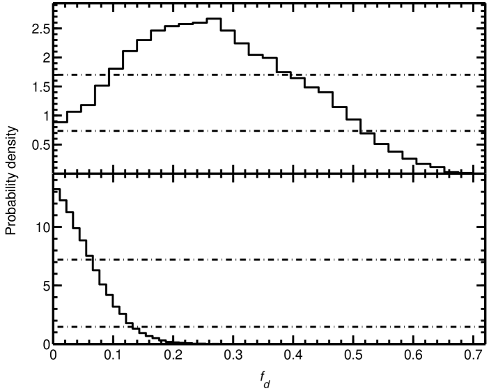
Figure 3: The marginalized likelihood function for the defect fraction when using only the WMAP data (top) and when additionally incorporating the BBN and HKP constraints (bottom). The horizontal lines show the 68% and 95% confidence levels.

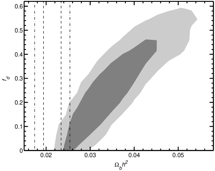
Figure 4: A plot of the likelihood from the fit to WMAP data projected onto the $\Omega_{\rm b}h^{2}$-$f_{\rm d}$ plane. The contours show the 68% and 95% confidence levels and highlight the degeneracy between the two parameters. The vertical lines show the 68% and 95% confidence limits of the determination of $\Omega_{\rm b}h^{2}$of Kirkman et al.

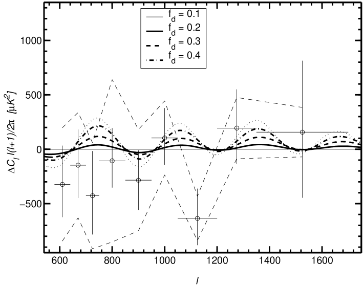
Figure 5: The changes to the temperature power spectrum for the same cases as in Fig. 2, but shown at higher multipoles and compared to the VSA data. The changes in the parameters follow the degeneracy present in the WMAP data but the changes in these previously unconstrained scales are too small for the VSA data to readily distinguish between the curves. The error bars do not include the 3% calibration uncertainty, which allows the power spectra values to be scaled up or down in unison. On this difference plot, this uncertainty is shown by the dashed zig-zags.

The use of other CMB data, on scales smaller than those probed by WMAP is an obvious first step toward applying further constraint to our model. Unfortunately, while each of ACBAR, CBI and VSA projects are capable of sub-WMAP resolution, they do not have the precision to limit the defect allowance to the point were the degeneracy is no longer a problem. This is illustrated in Fig. 5 for the VSA data. While of course their inclusion into our likelihood analysis does provide additional constraint, our results are almost unchanged by their addition and hence we shall not add unnecessary complication by discussing these data further.

A more direct way of limiting the degeneracy is to constrain the parameters $h$ and $\Omega_{\rm b}h^{2}$. As noted above, in applying a constraint on $h$ we are making our assumption of geometric flatness relevant and, therefore, we shall first consider $\Omega_{\rm b}h^{2}$. Big bang nucleosynthesis calculations give predictions for the primordial abundances of the light isotopes in terms of this parameter. However, it is not possible to directly measure these, only the abundances in astronomical objects at more recent times, and either assert that these abundances are representative of the primordial era or make some allowance for subsequent evolution. This is a notable problem and is perhaps responsible for there being discrepancies between $\Omega_{\rm b}h^{2}$ calculated using each of these isotopes. However, deuterium absorption lines have been seen in the spectra of a number of quasars, corresponding to the presence of gas clouds at high redshift. These low (but finite) metallicity clouds are believed to have experienced negligible deuterium processing and indeed show no notable correlation between metallicity and deuterium abundance Kirkman et al. (2003); Pettini and Bowen (2001). Unfortunately, the number of such clouds that have been well observed remains small and a number of difficulties exist in extracting the D/H ratio. Indeed, the spread in the measurements is a little large considering the estimated errors and Kirkman et al. Kirkman et al. (2003) conclude that it most likely as a result of uncertainty under-estimation rather than any real variation. They proceed to take the weighted mean of the log(D/H) measurements from five such systems but use the spread in the values to provide the uncertainty estimate. Their result is a value for $\Omega_{\rm b}h^{2}$ of $0.0214\pm 0.0020$, which we use here. However, it should be noted that uncertainties also arise from the use of nuclear cross-section data and that these can change this result slightly Cyburt (to be published).

Assuming a Gaussian form for the uncertainty, it is straightforward to add such data to the MCMC approach, for it simply adds a Gaussian term that multiplies the likelihood calculated from the WMAP data. As would be expected considering Fig. 4, its application is successful in limiting the effect of the degeneracy; however, the result of $\Omega_{\rm b}h^{2}=0.0245\pm 0.0014$ is still a little high. This is due to the WMAP data favoring a non-zero defect fraction, but once the BBN data is taken into account, the preference for defects is removed. The marginalized likelihood function for $f_{\rm d}$ is now highly skewed with its peak at the zero-defect limit. We therefore present merely the 95% confidence upper bound: $f_{\rm d}<0.14$ for case of the WMAP data with the BBN constraint. We estimate the MCMC uncertainty in this figure using the standard deviation between the values from the 5 independent chains, reduced by $\sqrt{5-1}$, and find that this gives $0.002$ in this case. The Hubble constant is constrained to $h=0.80\pm 0.08$, although a direct interpretation of this value as $h$ would assume flatness, while the results for rest of the parameters are shown in Table 2.

	BBN	HKP	BBN and HKP
$h$	$0.80\pm 0.08$	$0.80\pm 0.06$	$0.76\pm 0.05$
$\Omega_{\rm b}h^{2}$	$0.0245\pm 0.0014$	$0.0267\pm 0.0021$	$0.0242\pm 0.013$
$\Omega_{\rm m}h^{2}$	$0.126\pm 0.018$	$0.140\pm 0.015$	$0.134\pm 0.014$
$z_{\rm r}$	$13\pm 5$	$15\pm 5$	$13\pm 4$
$10^{10}A_{\rm s}^{2}$	$22\pm 3$	$23\pm 3$	$22\pm 2$
$n_{\rm s}$	$1.03\pm 0.04$	$1.07\pm 0.05$	$1.01\pm 0.03$
$f_{\rm t}$	$<0.26$	$<0.22$	$<0.19$
$f_{\rm d}$	$<0.14$	$<0.23$	$<0.13$

Table 2: Parameter values when constrained by the BBN and/or HKP results in addition to the first-year WMAP data (see Sec. III for definitions). Uncertainties indicated are standard deviations except for $f_{\rm t}$ and $f_{\rm d}$ for which 95% upper bounds are shown.

If the assumption of flatness is made explicit and the Hubble Key Project result of $h=0.72\pm 0.08$ Freedman et al. (2001) is applied instead of the BBN constraint, then the result is broadly the same. However, while $h$ is slightly more constrained in this case, $\Omega_{\rm b}h^{2}$ is less so and the upper bound on the defect contribution is rather higher, now: $f_{\rm d}<0.22$ (95% confidence, 0.003 MCMC uncertainty). However, this case does provide a bound that is independent of the BBN constraint, which we otherwise rely very heavily upon. If the two constraints are applied together, then the BBN data dominate and the result is essentially the same as when the BBN constraint was applied alone: $f_{\rm d}<0.13$ (95% confidence, 0.004 MCMC uncertainty). However, a number of the other parameters are more tightly constrained than in the previous case, most notably the tensor fraction. The effect of these constraints on the marginalized likelihood function for the defect fraction is shown in Fig. 3, with the final result being peaked at $f_{\rm d}=0$. The levels of defect and tensor contributions that correspond to the individual 95% upper bounds in this constrained case are those that were illustrated in Fig. 1.

While both defects and tensors contribute most to large scales, tensors do so almost exclusively for $\ell<100$ and so the effects of the two contributions are quite different. For example, while tensors suffer from a degeneracy similar to that for $A_{\rm d}^{2}$, in the tensor case there is an additional coupling to $\Omega_{\rm m}h^{2}$. Also there is a stronger coupling to $h$, as highlighted by the tensor contribution being more constrained once the HKP result is incorporated. However, as a result of there being some similarity in the two contributions, having a large tensor contribution does limit the degree to which defects are allowable and vice versa. But as neither the defect or tensor contributions can be negative, adding an additional degree of freedom by allowing defects, and so giving a positive expectation value for $A_{\rm d}^{2}$, further constrains $A_{\rm t}^{2}$, rather than allowing it greater freedom. The reverse is also true, such that if we disallow primordial tensors in our model, then the defect allowance increases a little. The percentage increase in $f_{\rm d}$ is about 15% in the two cases involving the BBN constrain and about 10% in the case when the HKP constraint was applied alone.

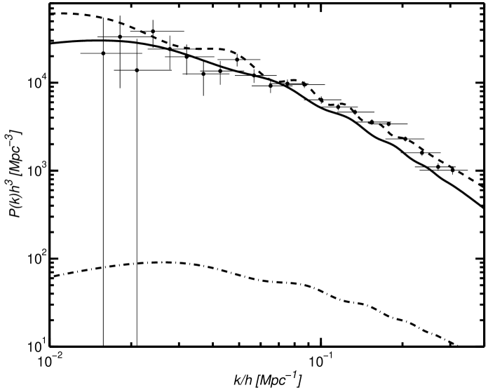
Figure 6: The current matter power spectrum in the non-defect case of Table 1 (solid line) compared to that for the $f_{\rm d}=0.4$ case (dashed line). The SDSS data is over plotted, showing an inability to distinguish the two cases. The sub-dominant defect contribution to the second case is also shown as the dot-dashed line.

As explained in the Introduction, we have not used the matter power spectrum to constrain our model because of uncertainty about the details of structure formation with global defects, caused by the non-Gaussianity of the perturbations. That non-Gaussianity can be important was shown in Ref. Avelino and Liddle (2004), where a model of cosmic string-induced perturbations Wu et al. (2002); Avelino et al. (1998) was studied and estimated to contribute less than around 1% of the total matter power spectrum at $8h^{-1}$ Mpc. The effect of the non-Gaussianity was to make re-ionization earlier and slower than in Gaussian models. While it is therefore inconclusive to simply compare the matter spectra, it is still interesting. Figure 6 compares one of the possible data sets, the SDSS data, with the $f_{\rm d}=0.0$ and $0.4$ cases from Table 1. The difference between the two cases is partially due to the added defect contribution, but is also due to the change in the cosmological parameters required to maintain the fit to the WMAP data. It is tempting to conclude that the SDSS data is not readily capable of constraining the defect degeneracy and hence the limitation of the degeneracy would again be dominated by the BBN constraint, but a definitive conclusion requires much more work on the matter power spectrum in models with global defects. Thus, we remain with our conservative position with regard to the use of large-scale structure data and have not incorporated it into our numerical results.

IV Discussion and Conclusions

We have found that in order to constrain the extent to which global defects assisted the seeding of cosmic structure, extra data in addition to the CMB temperature power spectrum must be used, or we require a greater knowledge of the spectrum than we have at present. This is despite the uncertainties in the WMAP data set used being dominated by cosmic-variance over the range where the defect contribution to the power spectrum is greatest. The freedom in the cosmological parameters and the primordial power spectrum are sufficient to allow a significant defect contribution while still fitting the data. It is only when parameters such as the physical baryon density and the Hubble parameter are restricted, via alternative astronomical techniques, that our model is significantly constrained. Then we find that the temperature power spectrum at a multipole of $\ell=10$ may have a fraction of 0.13 attributed to defects (95% confidence). The uncertainty in this upper bound that comes from the MCMC approach is 3%. More importantly, the numerical errors in the defect calculation are believed to be of order 10%, in which case there may be of order 10% change in this result. Also, if the primordial tensor component was removed then this result would increase by about 15%. In addition, this bound is quite sensitive to BBN result for the value for the physical baryon fraction $\Omega_{\rm b}h^{2}$ used and there has yet to be full agreement in this value among authors.

A further result of the degeneracy found is that, if defects were to contribute to cosmic structure formation, then there would a change in the values of the cosmological parameters estimated from the current CMB data. Most notably this affects $\Omega_{\rm b}h^{2}$, $h$ and $n_{\rm s}$ all of which are subject to an increase upon the addition of defects. This acts to re-enforce the more general point that any inferences made about the cosmological parameters from the WMAP data are model dependent and should be treated with caution.

We note that only a single defect type and model has been used in this investigation: textures resulting from the breaking of an $O(4)$ symmetry. However, the contributions from other global defect models are broadly the same as that considered here, although their spectra are by no means identical. Considering the $O(N)$ class of models for $N=2$ (strings), 3 (monopoles), 4 (textures) and 5 (non-topological textures) there is a gradual variation with $N$ of the relative contributions at low multipoles ($\ell\sim 10$) and high multipoles ($\ell\sim 300$), with strings giving preference to the latter Pen et al. (1997). This is likely to reduce the fractional contribution allowed from strings by perhaps 30% at $\ell=10$. Local defects in the form of cosmic strings may give a broad peak at $\ell\sim 400$ Battye and Weller (2000); Contaldi et al. (1999), beyond the first acoustic peak, and hence the results may be quite different.

Further, we wish to point out that the WMAP project is ongoing and new data with reduced uncertainties, as well as the addition of the EE polarization power spectrum, will be released. While the defect contribution to the EE spectrum is likely to be significant at only at large scales, the freedom for defects when using the CMB power spectra alone will be lessened by these data. It may be, however, that the Planck satellite pla is required to really explore sub-dominant defect contributions using these power spectra independently of other data. This mission will give precise temperature power spectrum measurement at sub-WMAP resolutions. It will also detect the B-mode polarization, which would be produced by the vector and tensor components of the defect perturbations. Finally, the non-Gaussianity of defect-induced perturbations has not been satisfactorily addressed, either in the matter power spectrum or the CMB. This may lead to more sensitive tests of defect scenarios.